Bi-criteria Algorithm for Scheduling Jobs on Cluster Platforms

Abstract

We describe in this paper a new method for building an efficient algorithm for scheduling jobs in a cluster. Jobs are considered as parallel tasks (PT) which can be scheduled on any number of processors. The main feature is to consider two criteria that are optimized together. These criteria are the makespan and the weighted minimal average completion time (minsum). They are chosen for their complementarity, to be able to represent both user-oriented objectives and system administrator objectives.

We propose an algorithm based on a batch policy with increasing batch sizes, with a smart selection of jobs in each batch. This algorithm is assessed by intensive simulation results, compared to a new lower bound (obtained by a relaxation of ILP) of the optimal schedules for both criteria separately. It is currently implemented in an actual real-size cluster platform.

1 Introduction

1.1 Cluster computing

The last few years have been characterized by huge technological changes in the area of parallel and distributed computing. Today, powerful machines are available at low price everywhere in the world. The main visible line of such changes is the large spreading of clusters which consist in a collection of tens or hundreds of standard almost identical processors connected together by a high speed interconnection network [6]. The next natural step is the extension to local sets of clusters or to geographically distant grids [10].

In the last issue of the Top500 ranking (from November 2003 [1]), 52 networks of workstations (NOW) of different kinds were listed and 123 entries are clusters sold either by IBM, HP or Dell. Looking at previous rankings we can see that this number (within the Top500) approximately doubled each year.

This democratization of clusters calls for new practical administration tools. Even if more and more applications are running on such systems, there is no consensus towards an universal way of managing efficiently the computing resources. Current available scheduling algorithms were mainly created to provide schedules with performance guaranties for the makespan criterion (maximum execution time of the last job), however most of them are pseudo-polynomial, therefore the time needed to run these algorithms on real instances and the difficulty of their implementation is a drawback for a more popular use.

We present in this paper a new method for scheduling the jobs submitted to a cluster inspired by several existing theoretically well-founded algorithms. This method has been assessed on simulations and it is currently tested on actual conditions of use on a large cluster composed by 104 bi-processor machines from Compaq (this cluster – called Icluster2 – was ranked 151 in the Top500 in June 2003).

To achieve reasonable performance within reasonable time, we decided to build a fast algorithm which has the best features of existing ones. However, to speed up the algorithm a guaranteed performance ratio cannot be achieved, thus we concentrate on the average ratio on a large set of generated test instances. These instances are representative of jobs submitted on the Icluster [18].

1.2 Related approaches

Some scheduling algorithms have been developed for classical parallel and distributed systems of the last generations. Clusters introduce new characteristics that are not really taken into account into existing scheduling modules, namely, unbalance between communications and computations – communications are relatively large – or on-line submissions of jobs.

Let us present briefly some schedulers used in actual systems: the basic idea in job schedulers [13] is to queue jobs and to schedule them one after the other using some simple rules like FCFS (First Come First Served) with priorities. MAUI scheduler [14] extends the model with additional features like fairness and backfilling.

AppleS is an application level scheduler system for grid. It is used to schedule, for example, an application composed of a large set of independent jobs with shared data input files [4]. It selects resources efficiently and takes into account data distribution time. It is designed for grid environment.

There exist other parallel environments with a more general spectrum (heterogeneous and versatile execution platform) like Condor [16] or with special capabilities like processus migration, requiring system-level implementation like Mosix [3]. However, in these environments scheduling algorithms are online algorithms with simple rules.

1.3 Our approach

As no fast and flexible scheduling systems are available today for clusters, we started two years ago to develop a new system based on a sound theoretical background and a significant practical experience of managing a big cluster (Icluster1, a 225 PC machine arrived in 2001 in our lab). It is based on the model of parallel tasks [9] which are independent jobs submitted by the users.

We are interested here in optimizing simultaneously two criteria, namely the minsum ($\Sigma C_{i}$) which is usually targeted by the users who all want to finish their jobs as soon as possible, and the makespan ($C_{max}$) which is rather a system administrator objective representing the total occupation time of the platform.

There exist algorithms for each criterion separately; we propose here a bi-criteria algorithm to optimize the $C_{max}$ and $\Sigma C_{i}$ criteria simultaneously. The best existing algorithm for minimizing the makespan off-line (all jobs are available at the beginning) has a $3/2+\epsilon$ guaranty [7]. We can derive easily an on-line batch version by using the general framework of [21] leading to an approximation ratio of $3+\epsilon$. For the other criterion, the best result is $8$ for the unweighted case and $8.53$ for the weighted case [19]. Using a nice generic framework introduced by Hall et al.[12], a ($12$;$12$) approximation can be obtained at the cost of a big complexity which impedes the use of such algorithms.

The paper is organized as follows: In the next section, we will introduce the definitions and models used in all the paper. The algorithm itself is described in section 3, along with the lower bound which is used in the experiments. The experimental setting and the results are discussed in section 4. Finally we will conclude in section 5 with a discussion on on-going works.

2 Context and Definition

2.1 Architectural and Computing Models

The target execution support that we consider here is a cluster composed by a collection of a medium number of SMP or simple PC machines (typically several dozens or several hundreds of nodes). The nodes are fully connected and homogeneous.

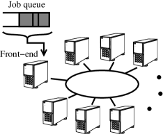
Figure 1: Job submission in clusters.

The submissions of jobs is done by some specific nodes by the way of several priority queues as depicted in Figure 1. No other submission is allowed.

Informally, a Parallel Task (PT) is a task that gathers elementary operations, typically a numerical routine or a nested loop, which contains itself enough parallelism to be executed by more than one processor. We studied scheduling of one specific kind of PT, denoted as moldable jobs according to the classification of Feitelson et al. [8]. The number of processors to execute a moldable job is not fixed but determined before the execution, as opposed to rigid jobs where the number of processors is fixed by the user at submission time. In any case, the number of processors does not change until the completion of the job.

For historical reasons, most of submitted jobs are rigid. However, intrinsically, most parallel applications are moldable. An application developer does not know in advance the exact number of processors which will be used at run time. Moreover, this number may vary with the input problem size or number of available nodes. This is also true for many numerical parallel libraries. The main exception to this rule is when a minimum number of processors is required because of time, memory or storage constraints.

The main restriction in a systematic use of the moldable character is the need for a practical and reliable way to estimate (at least roughly) the parallel execution time as function of the number of processors. Most of the time, the user has this knowledge but does not provide it to the scheduler, as it is not taken into account by rigid jobs schedulers. This is an inertia factor against the more systematic use of such models, as the users habits have to be changed.

Our algorithm proposes, thanks to moldability, to efficiently decrease average response time (at the users request) while keeping computing overhead and idle time as low as possible (at the system administrators request).

2.2 Scheduling on clusters

The main objective function used historically is the makespan. This function measures the ending time of the schedule, i.e., the latest completion time over all the tasks. However, this criterion is valid only if we consider the tasks altogether and from the viewpoint of a single user. If the tasks have been submitted by several users, other criteria can be considered. Let us present briefly the two criteria:

• Minimization of the makespan ($C_{max}=max(C_{j})$ where the completion time $C_{j}$ is equal to $\sigma(j)+p_{j}(nbproc(j))$). $p_{j}$ represents the execution time of task $j$, $\sigma$ function is the starting time and $nbproc$ function is the processor number (it can be a vector in the case of specific allocations for heterogeneous processors).

• Minimization of the average completion time ($\Sigma C_{i}$) [20, 2] and its variant weighted completion time ($\Sigma\omega_{i}C_{i}$). Such a weight may allow us to distinguish some tasks from each other (priority for the smallest ones, etc.).

In a production cluster context, the jobs are submitted at any time. Models were the characteristics of the tasks (duration, release date, etc) are only known when the task is submitted are called on-line as opposed to the off-line models were all the tasks are known and available at all times. It is possible to schedule jobs on-line with a constant competitive ratio for $C_{max}$. The idea is to schedule jobs by batches depending on their arrival time. An arriving job is scheduled in the next starting batch. This simple rule allows constant competitive ratio in the on-line case if a single batch may be scheduled with a constant competitive ratio $\rho$.

Roughly, the last batch starts after the last task arrival date. By definition, all the tasks scheduled in a batch are scheduled in less than $\rho C_{max}^{*}$, where $C_{max}^{*}$ is the optimal off-line makespan of the complete instance. The length of the previous last batch is then lower than $\rho C_{max}^{*}$. Moreover, the length of the last batch, plus the starting time of the previous last batch (at which none of the tasks of the last batch were released) is less than $\rho$ times the length of the optimal on-line makespan.

As the on-line makespan is larger than the off-line makespan, the total schedule length is less than $2\rho$ times the on-line optimal makespan. This is how the off-line $3/2+\epsilon$ algorithm is turned into an on-line $3+\epsilon$ algorithm as we said in the introduction.

3 A new bicriteria efficient solution

3.1 Rationale

Studying some extreme instances and their optimal schedules for the minsum criterion, gave us an insight on the shape of the schedules we had to build. For example, if all the tasks are perfectly moldable (when the work does not depend on the number of processors) the optimal solution is to schedule all the tasks on all processors in order of increasing area. This example shows that the minsum criterion tends to give more importance to the smaller tasks.

Previous algorithms presented in the literature are also designed to take into account this global structure of scheduling the smaller tasks first. Shmoys et al. [12] used a batch scheduling with batches of increasing sizes. The batch length is doubled at each step, therefore only the smaller tasks are scheduled in the first batches.

Existing makespan algorithms for moldable tasks are also designed with a common structure of shelves (were all tasks start at the same time) which is a relaxed version of batches. See for example [17] or [7] for schedules with 2 shelves.

Our algorithm was built with this structure in mind: stacking tasks in shelves of increasing sizes with the additional possibility of shuffling these shelves if necessary. However, our main motivation was to design a fast algorithm for the management of some clusters of a big regional grid in Grenoble. Our algorithm does not have a known performance guaranty on the worst cases, however we tested its behavior on a set of generated instances which simulate real jobs submitted on our local clusters. The principle of the algorithm is shown in Figure 2.

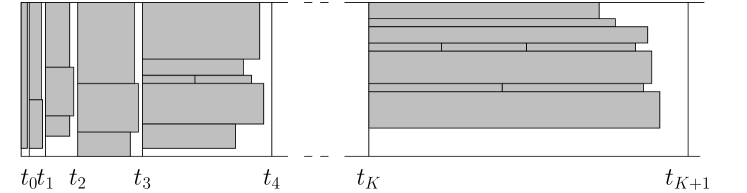
Figure 2: Principle of the algorithm.

3.2 Algorithm

More formally, we detail below the algorithm starting with the input describing the instances:

• $n$ tasks available at time $0$

• $p_{i}(k)$ the processing time of task $i$ on $k$ processors

• $w_{i}$ is its weight

• $m$ the number of processors

  Compute the approximate $C_{max}^{*}$ with the dual approximation algorithm.   $t_{min}=\min_{i,j}\{p_{i}(j)\}$   $K=\lfloor\log_{2}\left(\frac{C_{max}^{*}}{t_{min}}\right)\rfloor$   for $j=0..K+1$ do      $t_{j}=\frac{C_{max}^{*}}{2^{K-j}}$   end for   $T=\{1..n\}$   for $j=0..K$ do      $S=\{i\in T\mbox{ such that }\exists j,\ p_{i}(j)\leq t_{j}\}$      Merge the small sequential tasks sorted by decreasing weight.      Select the set $S_{j}\subseteq S$ of tasks to schedule in the current batch (using a knapsack).      Schedule the batch between $t_{j}$ and $t_{j+1}$.      Remove $S_{j}$ from $T$.   end for   Compact the schedule with a list algorithm using the batch ordering.

First, our algorithm calls a dual approximation makespan algorithm (defined in [7]) to determine an approximation of the optimal makespan of the instance. With this value $C_{max}^{*}$ and the smallest possible duration of a task $t_{min}$, we compute the smallest useful batch size $t_{0}$ (such that at least one task can be done) and $K+1$ the number of batches. The values $t_{j}$ are the length of our batches. For every $j$, $t_{j+1}$ is twice the value of $t_{j}$.

The main loop of the algorithm corresponds to the selection of the jobs to be scheduled in the current batch. We first select the tasks which are not too long to run in the batch. If there are several tasks that can be run in less than half the batch size on one processor, we can merge some of these tasks by stacking them together. In order to have as much weight as possible, this merge is done by decreasing weight order.

The next step is to run a knapsack selection, written with integer dynamic programming. We want to maximize the sum of the weight of the selected tasks while using at most $m$ processors. The allocation of the task $i$ is $allot_{i}$, the smallest allocation that fits (in length) into the batch. Values of $W(i,j)$ are initialized to $-\infty$ for $j<0$ and $0$ otherwise. For $i$ going from $1$ to $n$ and for $j$ going from $1$ to $m$, we compute:

$$W(i,j)=max\left(W(i-1,j),W(i-1,j-allot_{i})+w_{i}\right)$$

The largest $W(n,\cdot)$ is the maximum weight that can be done in the batch. The complexity of this knapsack is $O(mn)$.

The first schedule is simple: we start all the selected tasks of one batch at the same time. A straightforward improvement is to start a task at an earlier time if all the processors it uses are idle. A further improvement is to use a list algorithm with the batch ordering and a local ordering within the batches, as it allows to change the set of processors alloted to the tasks.

Finally, an additional optimization step is used. The batch order is shuffled several times and the best resulting compact schedule is kept. This only leads to small improvements.

The overall complexity of this algorithm is $O(mnK)$.

3.3 Lower Bound

In order to assess this algorithm with experiments, for each instance we need to know the value of an optimal solution. But since the problem is NP-Hard in the strong sense, computing an optimal solution in reasonable time is impossible. We are thus looking for good lower bounds.

For $C_{max}$ a good lower bound may easily be obtained by dual approximation [7]. For $\Sigma C_{i}$ the lower bound is computed by a relaxation of a Linear Programming formulation of the problem. This formulation is not intended to yield a feasible schedule, but rather to express constraints that are necessarily respected by every feasible schedule. For this formulation, we divided the time horizon into several intervals $I_{j}=(t_{j},t_{j+1}]$ with $0\leq j\leq K$. The values of the $t_{j}$ and the value of $K$ are defined as in the previous section.

Once the time division is fixed, we consider the decision variables $x_{i,j}=1$ if and only if task $i$ ends within $I_{j}$ (i.e. between $t_{j}$ and $t_{j+1}$), and $x_{i,j}=0$ otherwise.

For each task $i$ and each interval $j$, we can also compute the minimal area occupied by task $i$ if it ends before $t_{j+1}$:

$$S_{i,j}=\min_{1\leq k\leq m}\{kp_{i}(k)\mbox{ such that }p_{i}(k)\leq t_{j+1}\}$$

If the set is empty, let $S_{i,j}=+\infty$.

With these values, we can give the formulation of the problem:

$$\begin{array}[]{ll}\text{Minimize}&\sum_{i,j}w_{i}t_{j}x_{i,j}\\ \text{Subject to}&\forall i,\quad\sum_{j}x_{i,j}\geq 1\\ &\forall j,\quad\sum_{0\leq l\leq j}\sum_{i}S_{i,l}x_{i,l}\leq mt_{j+1}\\ &\forall i,\forall j,\quad x_{i,j}\in\{0,1\}\end{array}$$

The first constraint expresses that every task should be performed at least once. The minimization criterion implies that no task will be performed more than once: if $x_{i,j}$ and $x_{i,j^{\prime}}$ are equal to one, we get a better, yet still feasible solution by setting one of them to zero.

The second constraint is a surface argument. For each interval $I_{j}$, we consider the tasks that end before or in this interval (they end in $I_{l}$, for $l\leq j$). By definition, a task $i$ ending in interval $l$ takes up a surface at least $S_{i,l}$. The sum of all these surfaces has to be smaller than the total surface between time $0$ and time $t_{j+1}$, which is $mt_{j+1}$. This is obviously optimistic, because it does not take into account collisions between tasks: scheduling according to this formulation might require more than $m$ processors.

Both of these constraints are satisfied by every feasible schedules, so for every feasible schedule $S$, there is a solution $R$ to this linear program. Since for each job $i$, $\sum_{j}t_{j}x_{i,j}\leq C_{i}$, the objective function of $R$ is not larger than the minsum criterion of the schedule $S$. In particular, every optimal schedule yields a solution to the linear program, so the optimal value of the objective function is always smaller than the optimal value of the minsum criterion of the scheduling problem. This still holds when considering the relaxed problem, where $x_{i,j}$ is in $[0;1]$. The lower bound might be weaker, but is much faster to compute.

4 Experiments

4.1 Experimental setting

The experimental simulations presented here were performed with an ad-hoc program. Each experience is obtained by 40 runs; for each run tasks are generated in an off-line manner, then given as an input to the scheduling algorithm and to the linear solver which computes a lower bound for this instance. Comparison between the two results yields a performance ratio, and the average ratio for the whole set of runs is the result of the experiments.

The runs were made assuming a cluster of 200 processors, and a number of tasks varying from 25 to 400. In order to describe a mono-processor task, only its computing time is needed. A moldable task is described by a vector of $m$ processing times (one per number of processor alloted to the task). We used two different models to generate the tasks. The first one generates the sequential processing times of the tasks, and the second one uses a parallelism model to derive all the other values.

Two different sequential workload type were used: uniform and mixed cases. For all uniform cases, sequential times were generated according to an uniform distribution, varying from $1$ to $10$. For mixed cases, we introduce two classes : small and large tasks. The random values are taken with gaussian distributions centered respectively on 1 and 10, with respective standard deviations of 0.5 and 5, the ratio of small tasks being 70%.

Modeling the parallelism of the jobs was done in two different ways. In the first, successive processing times were computed with the formula $p_{i}(j)=p_{i}(j-1)\frac{X+j}{1+j}$, where $X$ is a random variable between $0$ and $1$. Depending on the distribution of $X$, tasks generated are highly parallel (with a quasi-linear speedup) or weakly parallel (with a speedup close to $1$). Respectively highly and weakly parallel are generated using gaussian distribution centered on 0.9, and 0.1, and with a standard deviation of 0.2. Any random value smaller than $0$ and larger than $1$ are ignored and recomputed. According to the usual parallel program behavior, this method generates monotonic tasks, which have decreasing execution times and increasing work with $k$. For the mixed cases, the small tasks are weakly parallel and the large tasks are highly parallel.

The second way of modeling parallelism was done according to a model from Cirne and Berman [5], which relies on a survey about the behavior of the users in a computing center. Only the $uniform(1,10)$ sequential time model is used for theses tasks.

To evaluate our algorithm, we use the lower bound (cf section 3.3) as reference. Some simple ”standard” algorithms are used to compare the behavior and efficiency of our approach.

Gang :

Each task is scheduled on all processors. The tasks are sorted using the ratio of the weight over the execution time. This algorithm is optimal for instances with linear speedup.

Sequential :

Each tasks is scheduled on a single processor. A list algorithm is used, scheduling large processing time first (LPTF).

List Graham:

All the 3 algorithms are multiprocessor list scheduling [11]. Every tasks is alloted using the number of processor selected by [7]. This should lead to a very good average performance ratio with respect to the $C_{max}$ criterion. Only the order of the list is changing between the three algorithms :

• the first one keep the order of [7], listing first task of the large shelf then the tasks of small shelf then the small tasks,

• weighted largest processing time first (LPTF), a classical variant, with a very god behavior for $C_{max}$ criterion, but the tasks are in fact sorted using the ratio between weighted and their execution time.

• smallest area first (SAF), almost the opposite of LPTF, the tasks are sorted according to their area (number of processors $\times$ execution time). The goal is to improve the average performance ratio for the $\sum w_{i}C_{i}$ criterion.

In all experiments, task priority is a random value taken from an uniform distribution between 1 and 10.

4.2 Simulation results

The results of the simulation runs are given in all the following figures, plotting the minimum, maximum and average values for $C_{max}$ and $\sum w_{i}C_{i}$. The average of the competitive ratio is computed by dividing the sum of the execution times over the sum of the lower bounds for every point [15]. Every workload type are represented separately. The same scale is represented for identical criterion between the workload type.

The tasks of Figure 3 are weakly parallel. This is the worst case for our algorithm as it spends resources to accelerate completion of small and high priority parallel tasks. These resources are thus spend without much gain. Note that Gang scheduling does not appear in the presented range for $C_{max}$, as Gang always has a very big ratio in this case.

As expected, the average performance ratio for our algorithm is worse than all other algorithms except Gang. Nevertheless, the performance ratio for $C_{max}$ is no more than $2$. All other algorithms have an average performance ratio around $1.5$. The difference is large enough to influence also the results for the minsum criterion. From this case we may deduce that for most cases, our algorithms will not be much worse than a performance ratio of $2$ for both criterion.

Figure 3: Performance ratio for the simulation on 200 processors, weakly parallel tasks

Figure 4: Performance ratio for the simulation on 200 processors, highly parallel tasks

Figure 5: Performance ratio for the simulation on 200 processors, mixed model parallel tasks

Figure 4 presents the same experiments with the highly parallel tasks. On the minsum criterion, our algorithm is clearly the best one. Gang and sequential have opposite behavior on both criteria, Gang being good with a small number of tasks and sequential good for a large number of tasks only. The other algorithms are stable (with respect to the number of tasks) but with a larger ratio on the minsum. Remark that the allotment computed for list algorithms is quite good, as $C_{max}$ performance ratio of these algorithms is always smaller than $2$.

The next experiment (cf Figure 5) presents mixed instances with some large tasks and plenty of small tasks. In this cases our algorithm is still quite stable with a performance ratio of around $2$ for both criterion, however SAF is better than our algorithm. The ratio of the two other list algorithms greatly increase with the number of tasks, which points out that the order of tasks is very important here.

Finally, the last experiment use a well known workload generator which emulates real applications [5]. In this more realistic setting our algorithm clearly outperforms the other ones for the minsum criterion, and is also the only one to keep a stable ratio for any number of tasks.

Several observations can be made from these results. First, the performance ratio for the minsum criterion is never more than $2.5$, and is on average around $2$. The performance ratio for the makespan is almost always below $2$, and is $1.9$ on average. This is very good, even for each criterion separately.

Figure 6: Performance ratio for the simulation on 200 processors, cirne model parallel tasks

The second observation is that our algorithm performs better when tasks are more parallel. This can be understood if we remark that, for a weakly parallel task, there is only one or two intervals in which it can be scheduled without degrading its performance. So the scheduling algorithm is more constrained when the tasks are not parallel.

The SAF algorithm perform quite well on simple cases. It appears on complex cases that our approach is required to keep a good performance on the minsum criterion. Thus our algorithms should be preferred in actual applications as its performance ratio for minsum is insensitive to jobs behavior and its performance ratio for the makespan is not far from alternatives.

Finally, Figure 7 shows that the execution time of our scheduling algorithm is low (less than 2 seconds for the largest instances), as expected.

Figure 7: Execution time of the algorithm.

5 Concluding remarks

In this paper we presented a new algorithm for scheduling a set of independent jobs on a cluster. The main feature is to optimize two criteria simultaneously. The experiments show that in average the performance ratio is very good, and the algorithm is fast enough for practical use. The algorithm has been assessed by comparing the minsum performance to a new lower bound based on the relaxation of an ILP, and comparing the makespan performance to the best known approximation. Actual results are not available at the moment, but we are currently implementing this algorithm on a full-scale platform (Icluster2).

Several technical problems still have to be solved for an even more efficient practical solution, namely the reservation of nodes which reduces the size of the cluster and the mix of different types of jobs (moldable jobs, rigid jobs, and divisible load jobs).

References

- [1] The top500 organization website. http://www.top500.org.
- [2] F. Afrati, E. Bampis, A. V. Fishkin, K. Jansen, and C. Kenyon. Scheduling to minimize the average completion time of dedicated tasks. Lecture Notes in Computer Science, vol. 1974, 2000.
- [3] A. Barak and O. La’adan. The MOSIX multicomputer operating system for high performance cluster computing. Future Generation Computer Systems, 13(4–5):361–372, Mar. 1998.
- [4] H. Casanova, G. Obertelli, F. Berman, and R. Wolski. The AppLeS parameter sweep template: User-level middleware for the grid. In Proceedings of SuperComputing’2000, Nov 2000.
- [5] W. Cirne and F. Berman. A model for moldable supercomputer jobs. In 15th Intl. Parallel & Distributed Processing Symp., 2001.
- [6] D. E. Culler, J. P. Singh, and A. Gupta. Parallel Computer Architecture: A Hardware/Software Approach. Morgan Kaufmann Publishers, inc., San Francisco, CA, 1999.
- [7] P.-F. Dutot, G. Mounié, and D. Trystram. Handbook of Scheduling, chapter Scheduling Parallel Tasks - Approximation Algorithms. CRC Press, 2004. chapter 28 of this book.
- [8] D. G. Feitelson. Scheduling parallel jobs on clusters. In R. Buyya, editor, High Performance Cluster Computing, volume 1, Architectures and Systems, pages 519–533. Prentice Hall PTR, Upper Saddle River, NJ, 1999. Chap. 21.
- [9] D. G. Feitelson and L. Rudolph. Parallel job scheduling: Issues and approaches. Lecture Notes in Computer Science, 0(949):1–18, 1995.
- [10] I. Foster and C. Kesselman. The grid: blueprint for a new computing infrastructure. Morgan Kaufmann Publishers Inc., 1999.
- [11] M. R. Garey and R. L. Graham. Bounds on multiprocessor scheduling with resource constraints. SIAM Journal on Computing, 4:187–200, 1975.
- [12] L. A. Hall, A. S. Schulz, D. B. Shmoys, and J. Wein. Scheduling to minimize average completion time: Off-line and on-line approximation algorithms. Mathematics of Operations Research, 22:513–544, 1997. \balancecolumns
- [13] R. L. Henderson. Job scheduling under the portable batch system. In D. G. Feitelson and L. Rudolph, editors, Job Scheduling Strategies for Parallel Processing, volume 949 of LNCS, pages 279–294, 1995.
- [14] D. Jackson, Q. Snell, and M. J. Clement. Core algorithms of the maui schedule. In D. G. Feitelson and L. Rudolph, editors, Job Scheduling Strategies for Parallel Processing, volume 2221 of LNCS, pages 87–102, 2001.
- [15] R. Jain. The art of computer systems performance analysis. John Wiley, New York, 1991.
- [16] M. J. Litzkow, M. Livny, and M. W. Mutka. Condor : A hunter of idle workstations. In 8th International Conference on Distributed Computing Systems (ICDCS ’88), pages 104–111, Washington, D.C., USA, June 1988. IEEE Computer Society Press.
- [17] G. Mounié, C. Rapine, and D. Trystram. Efficient approximation algorithms for scheduling malleable tasks. In Eleventh ACM Symposium on Parallel Algorithms and Architectures (SPAA’99), pages 23–32. ACM, juin 1999.
- [18] E. Romagnoli, Y. Denneulin, and D. Trystram. A synthetic workload generator for cluster computing. In 3rd International Workshop on Performance Modeling, Evaluation, and Optimization of Parallel and Distributed Systems (PMEO-PDS’2004) in conjunction with IPDPS’04, Santa Fe, New Mexico, 2004.
- [19] U. Schwiegelshohn, W. Ludwig, J. Wolf, J. Turek, and P. Yu. Smart SMART bounds for weighted response time scheduling. SIAM Journal on Computing, 28, 1998.
- [20] H. Shachnai and J. Turek. Multiresource malleable task scheduling to minimize response time. Information Processing Letters, 70:47–52, 1999.
- [21] D. Shmoys, J. Wein, and D. Williamson. Scheduling parallel machine on-line. SIAM Journal on Computing, 24(6):1313–1331, 1995.