Using matrices
in post-processing phase
of CFD simulations

Abstract

In this work I present a technique of construction and fast evaluation of a family of cubic polynomials for analytic smoothing and graphical rendering of particles trajectories for flows in a generic geometry. The principal result of the work was implementation and test of a method for interpolating 3D points by regular parametric curves and their fast and efficient evaluation for a good resolution of rendering. For the purpose I have used a parallel environment using a multiprocessor cluster architecture. The efficiency of the used method is good, mainly reducing the number of floating-points computations by caching the numerical values of some line-parameter’s powers, and reducing the necessity of communication among processes. This work has been developed for the Research & Development Department of my company for planning advanced customized models of industrial burners.

1 Introduction

Industrial and power burners have some particular requirements, as a customized study of the geometry for combustion head and combustion chamber for an optimal shape of the flame. Rapid prototyping for an accurate design of the correct geometry involves a numerical simulation of the gas or oil flows in the burner’s components (see Fig. 1).

Figure 1: Flows in combustion head (left) and combustion chamber.

The necessity of an high graphic resolution require a large amount of particles paths for tracing the streamlines of flow. Hence the numerical computation is memory and cpu very expensive for the used hardware environment. In a tipical simulation the number of paths to compute is some thousands, and the number of geometrical points to interpolate for each path is some thousands too. For the treatment of this large amount of data a parallel environment can be very useful.

2 Fitting trajectories with cubic polynomials

We suppose to have a dataset output from pre-processing and processing phases of a simulation, for example from numerical resolution of Navier-Stokes equations or from Cellular Automaton models [1]. We would a fast and flexible method to obtain from those data an accurate paths tracking of fluid particles with a smooth 3D visualization of trajectories, possibly with continuous slope and curvature. Our experience shows that Computational Fluid Dynamics packages have some limits in this post-processing phase, principally due to a rigid resolution of the initial mesh and to a small degree of parallelism.

Let S the number of 3D points for each trajectory and M the total number of trajectories from simulation dataset. We have tested that usual interpolation methods are have some disadvantages for our aims: for example Bezier-like is not realistic in case of twisting or diverging speed-fields; Chebychev or Least-Squares-like are too rigid for a customized application; polynomial fitting is simple but often shows spurious effects as Runge-Gibbs phenomenon [2]. We have elaborated a spline-based technique.

We suppose S = 4xN. For every group of four points, the interpolation is obtained by three cubic polynomials imposing four analytical conditions: passage at P_k point, $1\leq{k}\leq{3}$; passage at P_k+1 point; continuous slope at P_k point; continuous curvature at P_k point. For smooth rendering and for avoiding excessive twisting of trajectories, the cubics u_k are added to the Bezier curve b associated to the four points: v_k = $\alpha$b + $\beta$u_k, $0<\alpha,\beta<1$ (see Fig. 2).

Figure 2: Spline-based method with continuous slope and curvature.

In our simulations we have chosen $\alpha$ = $\beta$ = 0.5 . Let b = $As^{3}+Bs^{2}+Cs+D$, $0\leq{s}\leq{1}$, the Bezier curve of control points P₁, …, P₄, and let u_k = $at^{3}+bt^{2}+ct+d$, $0\leq{t}\leq{1}$, the spline between two points. One can see that the coefficients of this spline can be computed by a matrix-vector product coeff = T*p where coeff = ($a$, $b$, $c$, $d$), p = (P_k+1, P_k, $B$, $C$, 1) and T is a 4 x 5 numerical matrix, constant for every groups of points and for every trajectory. If we define the 4Mx5M global matrix

$${\bf G}=\left(\begin{array}[]{ccccc}{\bf T}&{\bf 0}&.&.&{\bf 0}\\ {\bf 0}&{\bf T}&.&.&{\bf 0}\\ .&.&.&.&.\\ .&.&.&.&.\\ {\bf 0}&{\bf 0}&.&.&{\bf T}\end{array}\right)$$

where 0 is a 4x5 zero-matrix, and define the vector s = (P_k+1, P_k, $B_{1}$, $C_{1}$, 1, …, P_k+1, P_k, $B_{\bf M}$, $C_{\bf M}$, 1), one can compute for every two-points group the coefficients of cubic splines for all the M trajectories with the matrix-vector product c = G*s. The matrix G is sparse with density equal at most to 1/M; if M = 1000, the density of 0.001 is a very good value for obtain the benefits of sparsity methods, mainly in computational total time and memory allocation [3].

3 Computing splines

For computing the coefficients of all the splines involved in the simulation, the complexity analysis shows a total number of operations of order M*N. Using P computational processes on a multiprocessor environment, a useful method is the distribution of M/P trajectories to every process. In this way every process receives M/P rows of the matrix G for computing splines by matrix-vector multiply. In a first experiment (fall 2003), we have used the Linux cluster at CINECA, Bologna (Italy), equipped with Pentium III 1.133 GHz processors, and a software environment constituted by C programs and MPI libraries [4]. The use of such parallel routines has been useful only for startup of multi- processes and data distribution. Tests have shown a quasi-linear speedup, in the sense of parallelism, for all the values of M and N respect to the number P of used processes (see e.g. Fig. 3).

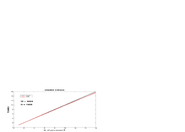
Figure 3: Speedup (red line) in computing splines coefficients using C routines and a Linux cluster.

In a second experiment (winter 2003), we have used a multinode Windows 2000 cluster of our company, equipped with a total of 4 Intel Xeon 3.2 GHz processors and 4 GB Ram, and a parallel environment using MATLAB 6.5 scripts on distributed package’s sessions on nodes. Tests have shown very high performances for splines computation using the internal algorithms of sparse matrix-vector multiply for the matrix G (see e.g. Fig. 4).

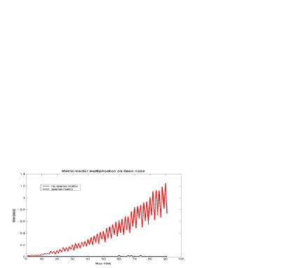
Figure 4: Total CPU-time for G*s matrix-vector multiplication on a Xeon 3.2 GHz node, using sparse (black line) and full (red line) matrix Matlab algorithm.

4 Valuating splines

After the computation of splines, we have focused on their valuations on a suitable set of parameter’s values. This set can be chosen large enough to obtain a fine sampling for an high graphic resolution. Consequently the amount of computation can be very huge, so that it is necessary an adequate method to valuate all the splines for all the trajectories.

Let V+1 the number of ticks for each spline valuation with a uniform sampling; then the ticks are (0, 1/V, 2/V, . . ., (V-1)/V, 1). The values of splines parameter t are (0, 1, 2, 3)-th degree powers of this array. The value of a cubic at t₀ can be view as a dot product:

$at_{0}^{3}+bt_{0}^{2}+ct_{0}+d=(a,b,c,d).(t_{0}^{3},t_{0}^{2},t_{0},1)$

This fact permits to consider the constant 4x(V+1) matrix

$${\bf T}=\left(\begin{array}[]{cccccc}0&(1/{\bf V})^{3}&.&.&(({\bf V}-1)/{\bf V})^{3}&1\\ 0&(1/{\bf V})^{2}&.&.&(({\bf V}-1)/{\bf V})^{2}&1\\ 0&(1/{\bf V})^{1}&.&.&(({\bf V}-1)/{\bf V})^{1}&1\\ 1&1&.&.&1&1\end{array}\right)$$

We consider the Mx4 matrix

$${\bf C}=\left(\begin{array}[]{cccc}a_{1}&b_{1}&c_{1}&d_{1}\\ a_{2}&b_{2}&c_{2}&d_{2}\\ .&.&.&.\\ .&.&.&.\\ a_{\bf M}&b_{\bf M}&c_{\bf M}&d_{\bf M}\end{array}\right)$$

where each row contains the coefficients of a spline interpolating two points in a single trajectory. Then the Mx(V+1) matrix product E = C*T contains in each row the values of a cubic between two data points, for all the M trajectories (eulerian view). In a similar way on can consider a lagrangian view for computing the values of all the cubics in a single trajectory. It can be easily shown that the total number of operations for computing all the values along each trajectory is of order NxMx(V+1).

5 Computing values of splines

For the computation of the values we have used the cluster of our company with multisessions of MATLAB package as parallel environment. It is fundamental for this step the improvement of performances due to the usage of LAPACK level 3 Blas routines incorporated in Matlab [5]. Another feature of this method is the fact that the matrix T is constant, hence it is computed only once, requires a small memory allocation so its values can be stored permanently in the cache. With P, number of processes, divisor of 3N, total number of two-points groups, the method used has been the distribution of 3N/P matrices C to every process.

The performances of multiprocess products show a quite linear speedup respect the P variable and a total computation time of order NxM; increasing the value of M or N for a better resolution, the time spent on computation doesn’t change if the value of processes is increased (Gustafson Law [6]) (see Fig. 5).

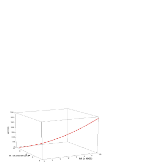
Figure 5: Total execution time for matrices products in the case 3N= 4200P.

6 Conclusions

These techniques have supplied good results for improving performances of post-processing phase in CFD simulations. Further work is planned for implementing a global matrix product for the splines evaluation, with the purpose of using the sparse matrices benefits to reduce total execution time and memory allocation.

References

- [1] G. Argentini. Message passing Fluids: molecules as processes in parallel computational fluids. In Recent Advances in Parallel Virtual Machine and Message Passing Interface: 10th European PVM/MPI Users’ Group Meeting, Venice, Italy, September 29 - October 2, 2003. Proceedings., LNCS 2840, Springer- Verlag, 2003.
- [2] A. Quarteroni, R. Sacco, F. Saleri. Numerical Mathematics, Texts in Applied Mathematics, Vol. 37, Springer-Verlag, 2000.
- [3] J.R. Gilbert, C.B. Moler, R. Schreiber. Sparse matrices in MATLAB: design and implementation. SIAM Journal of Matrix Analysis ad Application, 13(1), 1992.
- [4] www.cineca.it .
- [5] C.B. Moler. MATLAB Incorporates LAPACK. Increasing the speed and capabilities of matrix computation. MATLAB News & Notes, Winter 2000, www.mathworks.com/company/newsletters/news_notes/clevescorner/ winter2000.cleve.html .
- [6] P. Pacheco. Parallel programming with MPI, Morgan Kaufmann, 1997.