When Do Differences Matter? On-Line Feature Extraction Through Cognitive Economy

Abstract

For an intelligent agent to be truly autonomous, it must be able to adapt its representation to the requirements of its task as it interacts with the world. Most current approaches to on-line feature extraction are ad hoc; in contrast, this paper presents an algorithm that bases judgments of state compatibility and state-space abstraction on principled criteria derived from the psychological principle of cognitive economy. The algorithm incorporates an active form of Q-learning, and partitions continuous state-spaces by merging and splitting Voronoi regions. The experiments illustrate a new methodology for testing and comparing representations by means of learning curves. Results from the puck-on-a-hill task demonstrate the algorithm’s ability to learn effective representations, superior to those produced by some other, well-known, methods.

1 Introduction

Representation is the foundation for problem-solving: it provides the vocabulary and populates the world that we seek to understand and control. Although we can sometimes specify a good representation for particular problems, we have not understood the general learning problem until we understand how the representation can be learned along with the behaviors that lead to success in a task. There are also important practical reasons for studying autonomous representation learning. For example, success may depend on the agent’s ability to learn an effective representation from scratch if the task is poorly understood, or if there are too many possible scenarios for us to work out a complete specification of the state-space in advance. Even when it would be possible to design the representation beforehand, it might not be a cost-effective use of programmer time, especially if the representation will later need to be updated as the task environment changes.

This paper presents a new approach to the problem of autonomous representation learning, by applying the psychological principle of cognitive economy [19] to the domain of reinforcement learning [11, 21].

1.1 Effective representations

One of the hard problems facing any theory of cognition is that of finding principled ways of specifying when states of the world are “the same” and when they must be distinguished. Distinguishing every possible state of the world from every other state makes learning intractable except in very small, discrete state-spaces; but the agent cannot learn the task if the representation groups together states of the world that require different behaviors. Ideally, the agent should learn which states must be distinguished, while avoiding irrelevant distinctions that prevent it from generalizing its learning over states that are “the same kind of thing” in its task. How can an agent learn such a representation without knowing about the task beforehand?

1.2 Function approximation and value prediction

The typical approach to reinforcement learning represents the agent’s knowledge of the world in terms of an action-value function, $Q(s,a).$ This function gives the long-term estimate of reward that results from taking action $a$ from state $s,$ and following a greedy policy thereafter (that is, the agent chooses the action with the highest value in all subsequent states) [22, 21]. The original descriptions of Q-learning assumed a discrete representation: the action-value function was assumed to be stored as a table having a separate row for the values of each distinct state [22]. To extend the approach to large and continuous state-spaces, we may store the values $Q(s,a)$ more compactly as a parameterized function of $s$ and $a;$ the learning problem then becomes an exercise in function approximation, where the agent responds to its experiences in the world by adding features or tuning parameters so that it minimizes the mean-squared error (MSE) in the value predictions, $Q(s,a).$ Sutton and Barto comment that “our ultimate purpose is to use the predictions to aid in finding a better policy. The best predictions for that purpose are not necessarily the best for minimizing the MSE. However, it is not yet clear what a more useful alternative goal for value prediction might be,” [21, p. 196].

This paper presents an alternative goal for value prediction, based on the insight that some $Q$-value errors will have no effect on the agent’s ability to perform its task. The agent learns faster when it can generalize over “similar” states: states that agree on the preferred action and expectation of reward. Because similar states may differ on the expected values of non-preferred actions, grouping these states may increase the overall prediction error—even though these differences do not impact the agent’s performance in the task. In contrast, some states should be considered incompatible because ignoring their differences leads the agent to make bad decisions; such states must not be grouped together. This paper presents principled criteria for deciding when the differences matter and when they may be ignored.

1.3 Feature extraction and state abstraction

Assume a representational model in which the value function $Q$ is written in terms of a weighted set of feature detectors:

$$Q(s,a_{j})=\sum_{i}w_{ij}f_{i}(s)$$

This model characterizes much of the work on function approximation [21, Ch 8]. For example, we can describe a partition representation by defining a feature $f_{i}$ for each state-space region $S_{i},$ such that $f_{i}(s)=1$ for $s\in S_{i}$ and $f_{i}(s)=0$ for all all other states $s.$ This same model encompasses discrete (“look-up table”) representations, partition representations, tiled representations (such as CMAC [1]), perceptrons, and radial-basis function networks, depending on the definition of the $\{f_{i}\}.$

The features and the state-space regions lead to complementary ways of looking at the same function approximation process. We see that the function $f_{i}$ is a rule (intension) describing a set $S_{i}$ of states (extension) that are grouped together. We may define the state-space groupings in terms of the features, or equivalently, we may define the features in terms of the groupings. When the features $\{f_{i}\}$ are continuous-valued, the corresponding state groupings $\{S_{i}\}$ will be fuzzy sets. If we think of the state groupings as determining the feature detectors, we can think of the $S_{i}$ as “generalized states,” which determine how action values are stored—just as the individual states do in the discrete representation. This duality of features and state-space grouping is important because the grouping of states is the key concept for deciding which $Q$-value differences matter in the agent’s task. When we consider function approximation without discerning the role played by state abstraction, it becomes difficult to determine how the differences affect the agent’s ability to choose the correct behavior at each state.

1.4 Ad hoc approaches to state abstraction

One approach to representation is to continue to subdivide the state-space until its resolution is adequate to distinguish states that are not “the same kind of situation.” Ideally, the representation will make finer distinctions in parts of the space where the differences matter, and simplify the representation of other areas. In other words, the representation should have a resolution that varies throughout the state-space according to the demands of the task. Function approximation methods that simply cluster the task inputs cannot provide this kind of representation because they are blind with respect to the task requirements. Although we can sometimes specify important areas of the state-space for particular tasks, it is hard to do so in a general way.

For example, [10] assumed that states closest to the initial state required the finest resolution; [14] assumed that states closest to paths taken by the agent through the state-space were most important; [8] assumed that the most frequently-seen areas of state-space were most important. These criteria led to effective representations for the tasks being studied, but we can readily imagine tasks in which these criteria are irrelevant. We need representational criteria that explain why—and when—these strategies identify state-space differences that are relevant to the agent’s task. The key is to define important differences in terms of more general criteria for representational adequacy.

1.5 Cognitive economy

Cognitive economy generally refers to the combined simplicity and relevance of a categorization scheme or representation. Natural intelligences appear to adopt categorizations with high cognitive economy in order to make sense of the sea of stimuli impinging on their senses without overloading their bounded cognitive resources. Under the heading Cognitive Economy, Eleanor Rosch writes of the “common-sense notion” that the function of categorization is to “provide maximum information with the least cognitive effort,” “conserving finite resources as much as possible” [19, p. 28]. Then she writes (p. 29):

…one purpose of categorization is to reduce the infinite differences among stimuli to behaviorally and cognitively usable proportions. It is to the organism’s advantage not to differentiate one stimulus from others when that differentiation is irrelevant to the purposes at hand.

Cognitive economy results when the representation makes task-relevant distinctions while ignoring irrelevant information. This form of selective generalization presents the agent with a simpler working environment for its task. To apply this principle to reinforcement learning, we must define criteria for relevant distinctions without appealing to any task-specific information. This paper defines relevant distinctions in terms of the amount of reward that the agent stands to lose by ignoring them. The resulting criteria characterize state-space distinctions that are important for the agent to maximize its reward in the task. In this way, the task’s reward function determines relevance in the agent’s world.

2 Representational criteria

Given a pair of states, $s_{1}$ and $s_{2},$ we want to know whether the agent may safely group them together so that they share action values—will this state generalization cause the agent to lose reward? One way to find out is to consider the two states separately, comparing the expectation of reward for actions taken from $s_{1}$ with the expectations from $s_{2}.$ For example, we can consider the sum of the immediate reward given for taking action $a$ from $s_{1}$ and the value of the resulting state. In this way, we push our dependence on the value predictions one step into the future, and bypass any $Q$-value error caused by inappropriate generalization of $s_{1}.$ We may compare these “look-ahead” values with $Q(s_{1},a)$ in order to decide whether representational errors are compromising the agent’s ability to choose actions that maximize its reward in the task. We may also compare the look-ahead values for $s_{1}$ and $s_{2}$ in order to judge whether they may safely be included in the same “generalized state.” If not, the agent should refine its representation so that it learns their action values separately.

The next section presents a vocabulary for this discussion. Specifically, it defines value functions and action preference sets to be used in criteria for representational adequacy and state compatibility.

2.1 Preference and value functions

Definition 1 (Action value)

$$Q(s,a_{j})=\sum_{i}w_{ij}f_{i}(s)$$

This is the same definition given earlier, restated here for convenience.

Definition 2 (State value)

$$V(s)=\max_{j}Q(s,a_{j})$$

Thus $V(s)$ represents the long-term reward given by the best action available from $s.$ This is the standard definition of state value, given by [22, 21].

Definition 3 (Preferred action set)

$$\mbox{pref}_{\epsilon}(s)=\{a_{j}:Q(s,a_{j})\geq V(s)-\epsilon\}$$

The preferred action set contains the action or actions that appear to maximize the agent’s expected reward. Thus $\mbox{pref}_{0}(s)$ gives the action(s) with value $V(s),$ while taking $\epsilon>0$ makes the selection less stringent, and causes the preference set to contain all actions with value within $\epsilon$ of $V(s).$

The functions for our one-step look-ahead are analogous to the definitions of $Q,$ $V,$ and $\mbox{pref}_{\epsilon}(s).$

Definition 4 (Look-ahead action value, case 1)

Suppose that taking action $a$ from state $s$ always results in the following transition:

$$s\stackrel{{\scriptstyle a}}{{\longrightarrow}}r,s^{\prime}$$

Then we define

$$Q1(s,a)=r+\gamma V(s^{\prime})$$

Like the function $Q(s,a),$ $Q1(s,a)$ represents the expected discounted future reward when the agent chooses action $a$ from state $s.$ The parameter $\gamma$ is the Q-learning discount for future rewards [22, 21]. This definition holds when the task rewards and state transitions are deterministic.

Definition 5 (Look-ahead action value, case 2)

$$Q1(s,a)=\sum_{s^{\prime}}{\cal P}^{a}_{ss^{\prime}}[{\cal R}^{a}_{ss^{\prime}}+\gamma V(s^{\prime})]$$

In many tasks the rewards and state transitions will either be stochastic, or may appear stochastic simply because of imperfect function approximation. In this case, we need to modify Definition 4: we replace the immediate reward $r$ with its expected value, ${\cal R}^{a}_{ss^{\prime}},$ and we consider all possible resulting states $s^{\prime},$ weighted by their probability of occurrence, ${\cal P}^{a}_{ss^{\prime}}.$

Now we may define look-ahead versions of the state value and preference functions by replacing use of the value function $Q$ with $Q1$.

Definition 6 (Look-ahead state value)

$$V1(s)=\max_{j}Q1(s,a_{j})$$

Definition 7 (Look-ahead preferred action set)

$$\mbox{pref1}_{\epsilon}(s)=\{a_{j}:Q1(s,a_{j})\geq V1(s)-\epsilon\}$$

2.2 Representational adequacy

Definition 8 ($\epsilon$-adequacy)

Let $\delta$ be given, and assume that the agent always selects an action from $\mbox{pref}_{\delta}(s).$ We will say that a representation of the state-space is an $\epsilon$-adequate representation for $\delta\leq\epsilon,$ if for every state $s$ reachable by the agent, the following two properties hold:

$$\mbox{pref}_{\delta}(s)\subseteq\mbox{pref1}_{\epsilon}(s)$$ (1)

$$|V1(s)-V(s)|\leq\epsilon$$ (2)

Meeting the $\epsilon$-adequacy criterion guarantees that the state generalization at $s$ does not prevent the agent from being able to learn the correct policy at $s$ or mislead the agent at an earlier state as to the desirability of $s.$ Thus, this criterion defines a standard for representational accuracy at individual states, guaranteeing that the harmful effects of state generalization are kept in check and that the agent can learn to make sound decisions.

This standard defines an adequate representation as one that makes the distinctions needed for the task to remain learnable. It characterizes relevant distinctions in terms of the amount of reward that the agent stands to lose by ignoring them. This is the approach taken in [6], which introduces the incremental regret of a representation at time $t$—the amount of reward the agent loses when it groups its current state, $s_{t},$ in some category $S.$ A perfect representation would have an incremental regret of 0 at each step, because the representation would allow the agent to learn to distinguish the best action for every state.

Non-zero incremental regret arises from two kinds of representational error: grouping states that have different policies, and grouping states that have very different values. First, if the representation groups $s_{t}$ with the wrong states, the action that appears best for the group, $S,$ may be sub-optimal for $s_{t}.$ This could lead the agent to take the wrong action from $s_{t}.$ Second, if the value of $s_{t}$ is very different from the value of other states in $S,$ the agent might not recognize that arriving in $s_{t}$ is a special opportunity (or pitfall), because the action values are averaged over all the states in $S$—not just $s_{t}.$ This could cause the agent to make the wrong choice from $s_{t-1}.$ In both cases, the agent makes wrong decisions, resulting in lost reward in the task. The $\epsilon$-adequacy criterion limits the amount of lost reward by comparing the policy and value predicted by function approximation with the results of a one-step look-ahead. Thus the actions that appear to have the best value for $S$ must be good actions for $s_{t}$ (Equation 1, concerned with policy distinctions), and the state value of $s_{t}$ must be close to that predicted by the information given for the category $S,$ (Equation 2, for value distinctions). This bounds the incremental regret at $s_{t}$ by $\epsilon.$

The $\epsilon$-adequacy criterion allows us to take a representation for which the action values are known, and test whether it makes the state-space distinctions that are important for a particular task. If the action values are still being learned, such judgments are only provisional. It is useful to have an additional criterion for state compatibility, if the agent is to learn its representation along with the action values.

2.3 State compatibility

Although the $\epsilon$-adequacy criterion provides an objective standard for an adequate representation—one which allows the agent to learn its task—these characteristics of the representation are really the outcome of the particular distinctions the representation makes or fails to make between individual states. In practice, it is often more useful to be able to evaluate the compatibility of two states than the compatibility of a state with a region, because a poorly-chosen region could be incompatible with all its member states. This can also happen with good regions that simply have not had their action values updated for a long while.

Thus we need to bridge the gap between the high-level description of adequate representations and the low-level decisions the agent must make as to which states must be kept separate. In other words, when must the representation distinguish states and when may it generalize over states, in order for it to be $\epsilon$-adequate?

Definition 9 (State compatibility)

Let $\delta$ be given, and assume that the agent always selects an action from $\mbox{pref}_{\delta}(s).$ Assume that our goal is to produce an $\epsilon$-adequate representation, where $\epsilon\geq\delta.$

We will say that states $s_{1}$ and $s_{2}$ are compatible in case the following three conditions hold:

$$\mbox{pref1}_{\epsilon}(s_{1})=\mbox{pref1}_{\epsilon}(s_{2})$$ (3)

$$|V1(s_{1})-V1(s_{2})|\leq\delta$$ (4)

and

$$\mbox{pref1}_{\delta}(s_{1})=\mbox{pref1}_{\delta}(s_{2}) \mbox{ if }\delta\leq\epsilon/2$$ (5)

$$\mbox{pref1}_{0}(s_{1})=\mbox{pref1}_{0}(s_{2})$$ otherwise (6)

The criteria consist of three rules. The first rule ensures that the same actions appear desirable in each state. The second rule requires that the values of the states are close, based on a one-step look-ahead. The purpose of the third rule (Equations 5 and 6) is to ensure that the action which appears to be the best for a set of compatible states is, in fact, a pretty good action for any of the states in the set. This is difficult to guarantee when the compatibility criteria are written for pairs of states, rather than in terms of the whole set. That is why the criteria demand equality of the preference sets instead of merely requiring the preference sets to overlap. When $\delta\leq\epsilon/2,$ the looser restriction of Equation 5 allows the states to have slightly different values for the top actions, making the criteria more suitable for a practical algorithm which must account for real-world noise in the value estimates. The cut-off value of $\epsilon/2$ appears to come from the sum of the errors allowed by combining Equation 4 with Equation 5.

These issues are worked out in [6], which also offers a proof that for partition representations, separating incompatible states according to Definition 9 guarantees $\epsilon$-adequacy of the representation. Definition 9 thus describes criteria which are sufficient to produce $\epsilon$-adequate representations. The task of finding a set of necessary and sufficient conditions remains future work.

The representational criteria thus allow the system to detect relevant distinctions while generalizing over similar states. These criteria express the principle of cognitive economy in terms of representational adequacy and state compatibility. Since the criteria do this by examining the values of the actions available to the agent in its task, they allow feature extraction to proceed without depending on any other task-specific knowledge. In this sense, the approach is a principled one, and a solution to the general problem of representation learning by autonomous agents.

3 An Algorithm for On-Line Feature Extraction

The representational criteria not only provide a basis for understanding how accurately the action values must be learned, but these criteria also provide the means for analyzing and improving representations for a particular task. The most challenging application of these ideas is to learn the representation along with the rest of the task, especially when the system is forced to start from scratch, regarding the task environment as a black box. Here success depends on the integration of representation-learning with the rest of the system. In particular, learning the action values requires an adequate representation, yet the representational criteria depend on the accuracy of the (partially-learned) action values. Furthermore, changes made to the representation may cause additional changes in the action values. This section presents an online system that meets these challenges as it learns its representation along with the rest of the task. Although this system is just one possible implementation of the ideas, its success is an argument for the utility and robustness of the representational criteria.

The algorithm combines Q-learning [22] with an active strategy for remembering “surprising” states and examining them at the ends of trials. When the system’s current action leads to unexpected results, it pushes the current state on a replacing-stack data structure. (If the state belongs to the same region as an earlier state on the stack, the earlier state is removed). At the ends of trials, the system conducts mini-trials from the states on its stack, investigating the most recent surprising states first. These investigations produce action-value profiles which the system uses to update its action values, and also to determine whether the representation adequately represents the surprising states. If these states are not compatible with the prototype states for their regions, the system adjusts the state-space representation accordingly. The key differences from Q-learning are the use of the $\epsilon$-adequacy criterion (Definition 8) to detect surprising states, and use of the state compatibility criterion (Definition 9) to decide when to separate two states. In addition, this version of the algorithm sometimes selects starting states for its experiments on the basis of its stack, instead of always beginning at the same “start” state and proceeding to a terminal state.

The state-abstraction section of the algorithm is built upon a nearest-neighbor representation of the state-space. The partition regions are the Voronoi regions about each of a series of prototype states given to the representation. (A Voronoi region is the set of points closer to a particular prototype than to the other prototypes). Some regions consist of a single prototype and its Voronoi region, while others are compound regions consisting of a set of merged Voronoi regions. The compound regions are represented by a primary prototype state; this state is taken as the representative state for any of the states which fall in that region, even though some other state may be their nearest-neighbor prototype. If the state to be classified lies within a simple, un-merged region, its primary prototype will be the nearest-neighbor. When a state is judged incompatible with the prototype state for its region, we split the region by simply adding the surprising state as a new prototype; it then becomes the primary prototype of a new Voronoi region in the space.

3.1 The top level of the algorithm

The top level of the algorithm is given in Figure 1. It outlines the function get_action, which is called with the results of the transition

$$s_{t-1}\stackrel{{\scriptstyle a}}{{\longrightarrow}}r,s_{t}$$

$j\leftarrow$ region($s_{t-1}$) $k\leftarrow$ region($s_{t}$) if terminal($s_{t}$) or reliable_source($k$) then if terminal($s_{t}$) then $Q_{\mbox{new}}\leftarrow r$ else $Q_{\mbox{new}}\leftarrow r+\gamma\max_{i}Q(k,i)$ $Q(j,a)\leftarrow(1-\alpha)Q(j,a)+\alpha Q_{\mbox{new}}$ $\mbox{Updates}(j,a)\leftarrow\mbox{Updates}(j,a)+1$ if not $\epsilon$-adequate($s_{t-1}$) or $j$ has never been investigated or a weighted coin flip returns heads then push ($s_{t-1},j$) on the stack if terminal($s_{t}$) then process_stack() else return next_action()

Figure 1: get_action($s_{t-1},a,r,s_{t}$)

This function updates the action values and then calls a function to select the next action. The action value update is only applied when the new state, $s_{t},$ is considered reliable: the function ${\tt reliable\_source(k)}$ is true when $\mbox{Updates}(k,b)\geq$ MIN_UPDATES for some action $b.$ Rather than looking at the number of visits, this criterion determines whether any of the action values for region $k$ have been updated a certain minimum number of times. The value of MIN_UPDATES was $3$ for the experiments reported here. Checking for experience in this way is an enhancement that could be applied to any value iteration algorithm, and not essential to the algorithm.

The $\epsilon$-adequacy test done here to detect surprising states is a simplification of the one defined in Definition 8; it uses the simpler, non-stochastic definition of $Q1$ (Definition 4) to compare the recently experienced transition with the action-value profile $Q(j,\cdot).$

Typically, a driver process invokes get_action to begin a trial from some start state, $s_{0}.$ During a trial, the algorithm updates action values as Q-learning would, and then chooses the next action according to its current policy and action values. The algorithm continues to process state transitions fed to it by the driver, but may also initiate active exploration at the end of trials by invoking process_stack().

3.2 Active state investigations

while not empty( replacing-stack ) $s\leftarrow$ pop( replacing-stack ) $j\leftarrow$ region($s$) if FE_TIMER() then $\mbox{\tt update\_representation}(s,j)$ else investigate($s$) for each $a$: if reliable($a$) then $\mbox{Updates}(j,a)=\mbox{Updates}(j,a)+1$ $Q(j,a)\leftarrow$ $Q(j,a)$ $+\mbox{\tt alpha}(j,a)[Q1(s,a)-Q(j,a)]$

Figure 2: process_stack()

Figure 2 outlines the function process_stack(), which investigates states that appeared “surprising.” Because the stack is a last-in, first-out data structure, process_stack() explores states that occur at the ends of episodes before it explores earlier states. This property allows the system to focus on the frontier between unlearned states and states whose action values have already been grounded in the reward given by the environment. Actions leading to terminal states are learned first, then the action values of states one step earlier. As the system learns about states near the ends of trials, they stop being surprising, and the system focuses its attention on states which precede those states. In this way, the action values are learned from the end states backwards to the beginning states, but without all the extra action-value backups from internal states whose values have not yet been learned.

Because the stack is implemented as a replacing-stack, pushing any item causes the stack to remove any previous occurrence of that item before adding the new one. To enable the system to cope with continuous state-spaces, in which the same exact state might never be repeated, the stack regards states from the same region as “the same.” Therefore pushing a state removes any other states having the same region from the stack. This ensures that the stack size does not grow without bound: the number of items on the stack is limited by the number of state-space regions in the representation, and a particular region will not be explored more than once for any session. These are desirable qualities for cyclic tasks like the puck-on-a-hill task, because a single region might otherwise fill the stack with states seen during repeated passes through that region.

for each action $a$ $\hat{s}\leftarrow s$ $\hat{r}\leftarrow 0$ $\mbox{steps}=0;\;\mbox{discount}=1.0$ repeat $\hat{s}\stackrel{{\scriptstyle a}}{{\longrightarrow}}r,s^{\prime}$ $k\leftarrow\mbox{region}(s^{\prime})$ $\hat{r}\leftarrow\hat{r}+\mbox{discount}*r$ $\mbox{discount}=\gamma*\mbox{discount}$ steps $\leftarrow$ steps $+1$ $\hat{s}\leftarrow s^{\prime}$ until $\mbox{\rm region}(s^{\prime})\neq\mbox{region}(s)$ or $\mbox{steps}\geq\mbox{MAX\_STEPS}$ or terminal($s^{\prime}$) $\mbox{reliable}(a)\leftarrow\mbox{\tt reliable\_source}(k)$ if terminal($s^{\prime}$) then $Q1(s,a)\leftarrow\hat{r}$ else $Q1(s,a)\leftarrow\hat{r}+\gamma\max_{i}Q(k,i)$

Figure 3: investigate($s$)

The system investigates a state by conducting a mini-trial for each possible action from that state (Figure 3). These trials only last long enough for the agent’s state to enter another region or for it to reach a terminal state. In the case of an action that leads back to the same region, the investigation times out after a certain number of steps. If a single action takes the agent out of the region, the mini-trial stops after one action.

Feature extraction is not performed after every trial. If this investigation is not one in which the system will perform feature extraction, the system applies the results of its investigation by updating action values according to the new profile. Like the Q-learning updates done in the top level of the algorithm, these updates only back up values when the resulting states (from the investigations, in this case) are determined to be reliable. Unlike those updates, the learning rate for the active updates decreases with the number of times the action value has been updated, until it hits a specified minimum value (Figure 4).

if $\mbox{Updates}(j,a)\leq\mbox{ENOUGH\_SAMPLES}$ return $1.0/\mbox{Updates}(j,a)$ else return $1.0/\mbox{ENOUGH\_SAMPLES}$

Figure 4: alpha($j,a$)

3.3 State abstraction module

$s_{p}\leftarrow$ primary prototype for $s$ $s_{p2}\leftarrow$ n earest-neighbor prototype for $s$, (if $s_{p}$ isn’t nearest) investigate($s$) investigate($s_{p}$) update $Q(j,\cdot)$ by $Q1(s_{p},\cdot)$ if (should_split$(s,s_{p})=$ no) or (reliable_prototype$(j)=$ no) then update $Q(j,\cdot)$ by $Q1(s,\cdot)$ else split $j:$ reduce reliability info for $j$ if $s_{p2}$ exists then investigate($s_{p2}$) if ( should_split$(s_{p},s_{p2})=$ no) or (should_split$(s,s_{p2})=$ yes) then add $s$ as a new prototype if (should_split$(s_{p},s_{p2})=$ yes) then detach $s_{p2}$ from $s_{p}$ if we did not add $s$ as prototype update $s_{p2}$ with $Q1(s,\cdot)$ if MERGE_TIMER() then consolidate compatible states

Figure 5: update_representation($s,j$)

if (all actions are reliable from $s_{1},$ and all actions are reliable from $s_{2},$ and $\mbox{\tt compatible}(s_{1},s_{2})=$ no) then return yes else return no

Figure 6: should_split($s_{1},s_{2}$)

Figure 5 outlines the feature extraction algorithm, implemented by the function update_representation($s,j$). The timer FE_TIMER() causes this function to be invoked at regular intervals, allowing time for the action values to settle between changes to the representation (see Figure 2). The function reliable_prototype($j$) tests whether $Q(j,b)$ has been updated at least MIN_UPDATES times for every action $b;$ this is a stricter test than reliable_source($j$), which guards the action value update in the top level of the algorithm (Figure 1). The function compatible($s_{1},s_{2}$) applies the state compatibility criterion given in Definition 9, taking the value of $\delta=\epsilon.$

The basic idea is this: when investigating surprising states, if the current state appears to be incompatible with its classification because of a policy or value difference that results in significant lost reward, then add the state as the seed of a new state-space category. Occasionally, consider whether the representation may be simplified by merging compatible regions, and whether merged regions ought to stay merged.

3.4 Methodology

How should we test an algorithm for on-line feature extraction? We want to know whether the algorithm produces high quality representations for the agent’s task. A common test is to simply evaluate the performance of an agent that uses the algorithm to construct its representation for the task as it goes about learning the task. Although this technique is often seen in the literature, good performance in the task does not necessarily indicate a high quality representation; evaluating a representation is different from simply evaluating performance.

Several other criteria may help evaluate the quality of the representation. If the representation contains a small number of features, that may be taken as evidence of cognitive economy, provided that those features allow the agent to make the necessary distinctions in its task. If the representation is reusable by other agents, that is evidence that it captures important features of the task, rather than artifacts of a particular training regimen. If the representation allows good performance from a variety of starting points, that may indicate a high level of quality throughout the relevant parts of the state-space. Therefore, our evaluation methodology should test the representation independently of the system which produced it, and should exercise the representation over a significant portion of the state-space. Our quality assessment will be based on the number of features and the effectiveness of the representation in the task.

The effectiveness of the representation may be shown most effectively by a learning curve that plots task performance against training time for learning the action values. Learning curves are especially useful for evaluating representations, because a single measurement of either learning speed or performance is likely to mislead. A single measurement of learning speed tends to favor small representations, which have fewer parameters to be trained, while a single measurement of performance tends to favor large representations, which tend to learn more slowly but eventually produce superior performance. In addition, learning curves show whether a representation reliably supports good performance, or only results in occasional successes. If a learning curve is produced, it should be averaged from multiple experimental runs, in order to minimize system initialization effects. (Even though the algorithm may be deterministic, its implementation may rely on random numbers for action selection when its preferred action set contains more than one action).

The experiments reported here consisted of two stages: a representation generation stage and a representation testing stage. In the generation stage, a learning system applied the algorithm described above, constructing its representation as it learned the task. The output of this stage is the specification of a new state-space representation for the task. For the algorithm to succeed, it must not only learn to perform well in the task, but must produce a representation that captures the important features of the problem, in a form reusable by other agents.

The testing stage consisted of inserting the generated representation into another reinforcement learning system and producing learning curves for this new system. Although the representation is now fixed, the system must still learn its action values from scratch, which is why it improves with training. Since the tester is separate from the agent that produced the representation, it is able to evaluate different representations fairly, and it allows us to compare them in a way that controls for the other aspects of the reinforcement learning problem. This method of evaluating learned representations in a separate system appears to be unique.

To produce a learning curve, the system’s action values were reset, and the system generated a series of learning trials. The system’s performance was evaluated at the ends of trials, but not after every trial. It was important not to interrupt a running trial because the task studied here has rewards only at the ends of trials. At the end of a trial, deciding whether to generate a performance measurement depended on a two-part test: the system needed to have completed either a pre-set number of learning steps or a pre-set number of trials. This two-part test insured that the system generated enough data points both early in the run (when trials are short, so the number of trials dominates) and late (when trials are long, and the number of learning steps dominates).

Each performance measurement was the median score for a batch of trials from a set of random starting states. (For the puck-on-a-hill task reported here, the scores were just the trial lengths). The random starting states were chosen as follows. A preliminary series of experiments yielded a set of extreme values for the state-space coordinates; the tester’s training trials were started at states from the central third of this observed state-space, and its test trials were started at states from a slightly smaller zone—the central quarter of the space. Initializing trials at random starting states ensures that the representation is tested over a significant portion of the space, providing a more meaningful indication of the quality of the representation.

4 Case Study: Puck-On-A-Hill Task

The puck-on-a-hill is a bang-bang control task in which rewards are seen only at the ends of episodes that are normally very long (up to 5 million steps) and include tight cycles. Performance in this task depends on the adequacy of the state-space representation. A Q-learning agent performs poorly with some seemingly reasonable representations for this task; but analysis of the task leads to a simple, two-category representation that is optimal in a sense described below. Therefore, this is an effective demonstration task for evaluating algorithms for on-line feature extraction.

Figure 7: The puck-on-a-hill task

In the puck-on-a-hill task, the agent controls a puck which it must learn to push to the left or the right to keep the puck balanced on the top of a hill. The agent’s only reinforcement comes when the puck falls too far down the hill on either side and hits the containing wall. When that happens, the agent is given a reward of $-1,$ and the episode ends. This task has been studied previously in [9] (although with a slightly different form for the equations of motion) and in [6]. Figure 7 illustrates the task.

The puck-on-a-hill is similar to the familiar pole-balancing task [13, 2, 7] but with a two-dimensional state-space having components for position and velocity only. The simulation details are as follows.

State	$x$, position of puck (meters)
	$v$, velocity of puck (m / sec)
Control	$f$, force on puck (Newtons)
Constraints	$-2.4<x<2.4$
	$f=\pm 3.0$
Equation of hill	$y=-\beta x^{2}$
Parameters	$\beta=0.3$ (hill curvature)
	$g=9.8$ m / $\mbox{sec}^{2}$ (grav. accel.)
	$m=1.0$ kg (mass of puck)
	$\Delta=0.02$ sec,
	(sampling interval)

Positive $x$ represents a position on the right side of the hill. The corresponding angle of the cart with the hill is given by $\theta,$ where positive $\theta$ represents a position on the left side of the hill. Positive $f$ pushes the puck toward the right.

The equations of motion are as follows.

$$x(t+1) = x(t)+\Delta v(t)$$

$$v(t+1) = v(t)+\Delta\frac{(f(t)-mg\sin\theta(t))\cos\theta(t)}{m}$$

$$\theta(t) = \arctan(-2\beta x(t))$$

4.1 Analysis

Some analysis of the task will help us understand what makes for a good representation. The puck’s acceleration is determined by its thrusters and the downward pull of gravity. Near the center of the hill, the thrusters dominate the force of gravity: the puck can push itself back to the crest of the hill as long as its prior velocity is not too large. Away from the center, the hill’s slope becomes increasingly steep, so that gravity overwhelms the contribution of the puck’s thrusters. Therefore, once the puck has fallen too far down the hill, it loses the ability to climb back up, and fails shortly after.

Just where this “point of no return” lies depends on the puck’s velocity. From the equations of motion, we see that the acceleration on the puck is zero when

$$f(t)=mg\sin\theta(t)$$

$$\frac{f}{mg}=\sin\arctan(-2\beta x)$$

$$\frac{\tan\arcsin\frac{f}{mg}}{-2\beta}=x$$

Substituting the values of the parameters, $f=\pm 3.0\mbox{ Newtons, }g=9.8\mbox{ m}/\mbox{s}^{2},\beta=0.3,m=1.0\mbox{ kg},$ we have

$$x=\frac{\tan\arcsin\frac{\pm 3.0}{(1.0)(9.8)}}{(-2)(0.3)}\doteq\pm 0.54$$

At this point, a puck with zero velocity can hold its position on the hill; if we place a stationary puck farther out, it cannot avoid falling down the hill. On the other hand, if the puck is already moving up the hill, its existing velocity may be sufficient to carry it back into the controllable region, even starting from a point farther down the hill. Therefore, the “point of no return” lies farther down the hill with higher puck velocities.

The agent must keep the puck within the region where its thrusters are effective in controlling the puck. We will call these states controllable states, and we will call the states that are past a “point-of-no-return” doomed states. Figure 8 shows the controllable states, which form a band falling roughly diagonally through the middle of the state-space. This figure was produced by running puck experiments at each point of a very fine grid. (Resolution was 0.01 in both $x$ and $v$). The remaining states are all doomed states, from which the puck cannot avoid falling down the hill and hitting a wall, no matter what actions it takes.

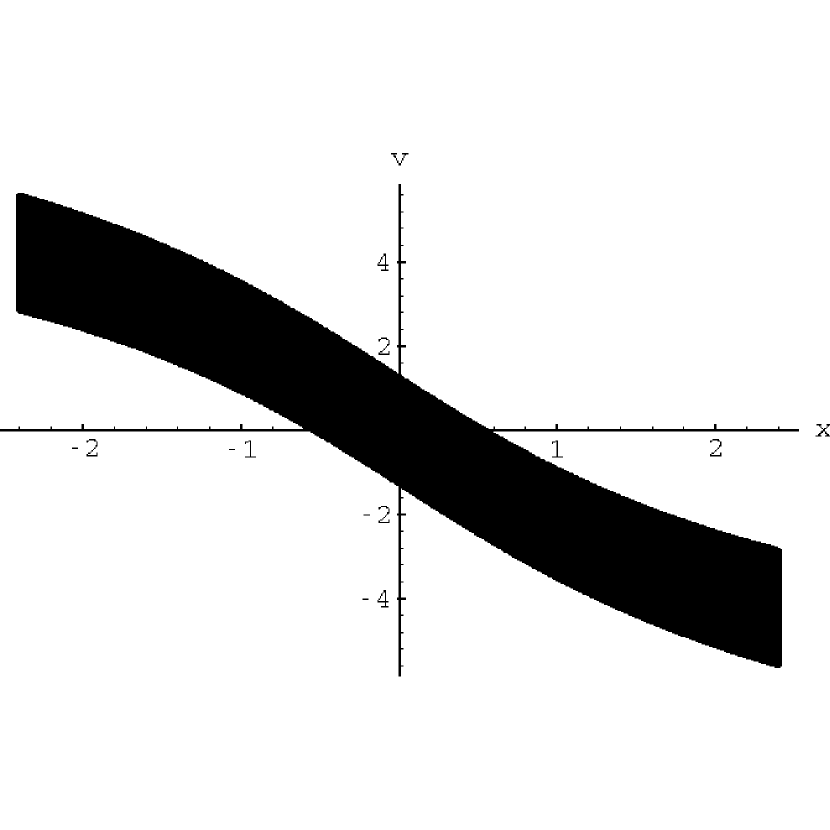
Figure 8: Controllable states: states outside this band result in failure.

Since hitting a wall is the only source of reinforcement in this task, the best possible return is $0,$ obtained by a policy that keeps the puck within the controllable zone. Any policy that does so is therefore an optimal policy for this task. If pushing right from a controllable state $s_{c}$ results in a doomed state, then we may classify $s_{c}$ as a “must-push-left” state. Similarly, if pushing left results in a doomed state, we may classify $s_{c}$ as a “must-push-right” state. If both left and right lead to other controllable states, we may classify $s_{c}$ as a “don’t care” state. The critical states are the must-push-right and must-push-left states, where the agent’s next action determines whether it succeeds in the task. These states are on the edges of the controllable zone; the states in the middle of the controllable zone are don’t-care states because neither action will push the puck past the boundary of the zone. Figure 9 shows the critical states: the must-push-left states make up the top curve, and the must-push-right states make up the bottom curve. These plots were determined by testing each controllable state found in the earlier simulation, evaluating the controllability of the states which result after a single push to the left or right.

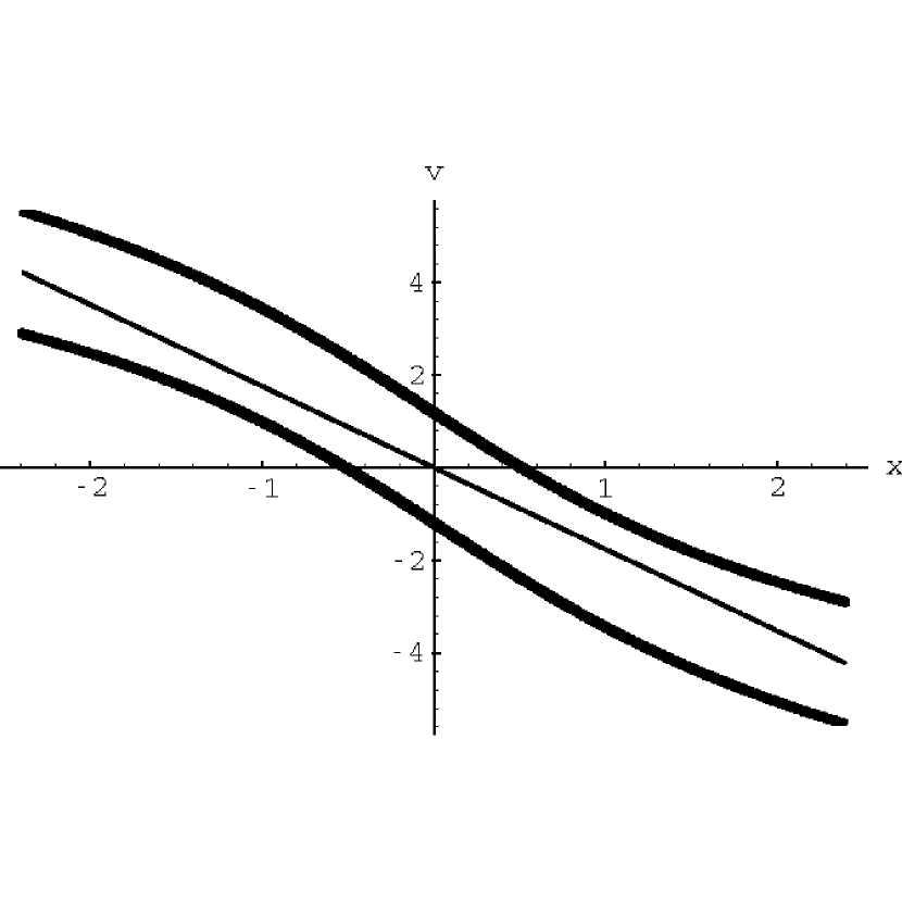
Figure 9: An ideal representation: must-push-left states (top curve) and must-push-right states (bottom curve) are separated by the diagonal line.

This analysis shows that simply pushing toward the center of the hill is not an optimal policy. For example, if the puck is moving fast enough toward the right, it may need to push to the left, even when it is already on the left side of the hill. Otherwise, it may be unable to slow down on the other side and avoid hitting the right wall. Any policy that pushes to the left in the must-push-left states (the top curve in Figure 9) and pushes to the right in the must-push-right states (the bottom curve) is an optimal policy. Therefore, any representation that separates these two classes of states will be adequate for learning an optimal policy. For example, we can simply bisect the controllable zone by the line $v=-1.7615x,$ (Figure 9). Since this representation cleanly separates the must-push-right states from the must-push-left states, it allows the system to learn an optimal policy. In addition, this is one of the simplest possible representations that preserves the necessary distinction. Therefore, this diagonal-split representation is a useful benchmark for evaluating other representations.

4.2 Results

The results compare the performance of a test system under different state-space representations. Each representation was evaluated by inserting it into the test system and generating a series of 10 learning curves, which were then averaged. The learning curves plot performance against the number of training steps experienced by the test system. Each performance score is the median trial length for a batch of 50 trials conducted with learning turned off. The test trials were stopped if they reached 5,000,000 steps. After 50,000 steps of training, the diagonal-split representation and the learned representation both attained averaged performance scores of 5,000,000 steps.

4.2.1 Generated representations

Starting from scratch, the system generated a representation consisting of 24 prototype states, shown in Figure 10. Although the prototypes have a slightly asymmetric layout, their placement allows the system to easily identify points that are closer to the “must-push-right” boundary than the “must-push-left” boundary, and vice versa. The system adds prototypes from states that it visits, sometimes in the later stages of a failing trial. The reason that the system kept generating points farther out from the center is most likely that it learned a more negative state value, $V1(s),$ for states closer to failure points. Although this value difference turned out to be unimportant in the puck task, there exist other tasks where it would have been a critical distinction.

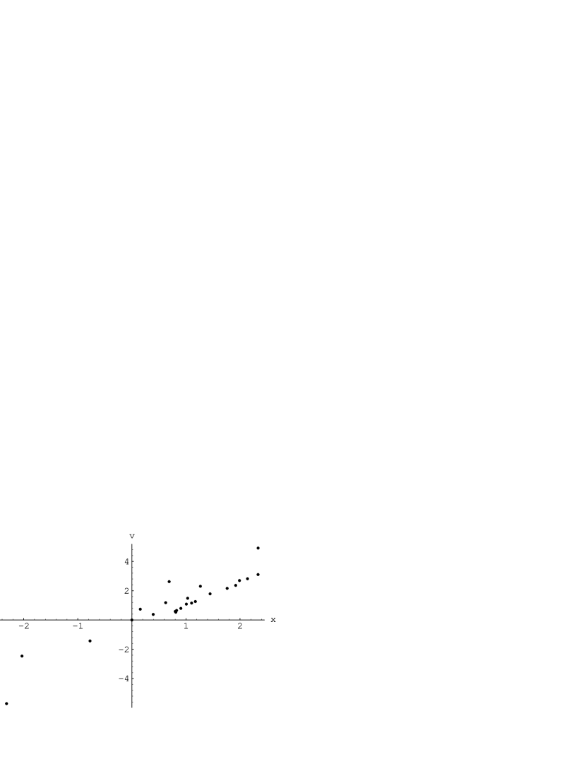
Figure 10: Representation constructed automatically, from scratch (24 categories).

In another experiment, the system was seeded with a representation consisting of the two $(x,v)$-space points (0.2680, 0.6200) and (-0.2680, -0.6200). These points are on either side of the controllable zone; although the line connecting them is not quite perpendicular to the line of the diagonal-split representation described earlier, these two points were thought to be sufficient to distinguish must-push-left points from must-push-right points. The objective of this second experiment was to verify that the state compatibility criteria do not lead to the generation of unnecessary states. This was confirmed by the resulting representation, which simply added two states at the usual failure points of the task. Figure 11 shows the representation. The learning process which produced it required 207 trials, with the last trial continuing for over 100 million steps.

Figure 11: Representation constructed from a good seed representation.

4.2.2 Control representations

The results compare the performance of the 24-category generated representation with the performance of four other representations: the diagonal-split representation described above, a uniform $10\times 10$ grid partitioning, a representation inspired by Variable Resolution Dynamic Programming [14], and a representation designed to maintain controllability [9].

Variable Resolution Dynamic Programming (VRDP) produces a partitioning of the state-space with the highest resolution at states visited during experimental trials. Away from these experimental trajectories, resolution falls off gradually according to a constraint on neighboring regions. The experimental trials are “mental practice sessions” conducted according to an internal model being learned by the agent. For the studies reported here, the representation was constructed from two trials using the puck task environment: an initial trial in which the agent always pushed to the right, and a successful trial in which the agent succeeded in keeping the puck in the center of the hill for over 100,000 steps. (The successful trial was taken from a system with the uniform $10\times 10$ partitioning of the space). Because VRDP initializes the representation to a single box, the initial trial consisted of selecting the same action repeatedly (since the policy for all states is the policy of that single box). When the representation was fine enough to allow good performance, mental practice sessions would focus on the states seen in the successful trial. Therefore, VRDP would be likely to visit the same points in mental practice sessions which were visited in the two experimental trials—and most likely, additional points as the representation was being learned and performance was still improving. Therefore, this representation is probably an idealized version of the application of VRDP to the puck task. As in [14], the highest resolution of each state-space coordinate was found by performing six binary splits of that coordinate. Taking the state-space dimensions to be $[-2.4,2.4]\times[-5.5,5.5],$ this resulted in the smallest distinctions being $\Delta x=4.8/64=0.075$ and $\Delta v=11.0/64=0.171875.$ Figure 12 illustrates the resulting representation.

Figure 12: A representation inspired by Variable Resolution Dynamic Programming.

Figure 13: Enhanced VRDP representation.

Unfortunately, this representation performed poorly, attaining a maximum averaged performance score of 2215 steps. (Both the diagonal-split representation and the generated representation achieved averaged scores of 5,000,000 steps). One reason for this poor performance may be that the partitioning is very fine along the path from the origin to the failure point of the first trial. As a result, reward from a failure must pass through a very long series of intermediate boxes before it reaches the critical states where the agent can actually control the puck. To test this explanation, I made a second VRDP-inspired representation, shown in Figure 13. Although this representation does not entirely observe the constraint on neighboring regions, it removes most of the boxes resulting from the initial failed trial. Since this representation performed much better than the original, it replaces the original VRDP representation in the comparison plots which follow.

The other representation, shown in Figure 14, was taken from [9]. This representation attempts to limit the agent’s loss of controllability, according to an off-line analysis computed in terms of a model of the task: First, compute the worst-case deviations between possible trajectories of the agent that start from different states; then divide the state-space into regions small enough that when this deviation is integrated over all pairs of states in a region, the resulting controllability error is less than a tolerance. This representation was part of an Adaptive Heuristic Critic system [3] which learned to balance the puck for over 10,000 steps, after an average of 13 trials and 2000 training steps. Since [9] assumed that trials always start at (0, 0), the experiments reported here may have been a more severe test of this representation than the original study, because my test system starts trials at randomly-chosen starting points.

Figure 14: Representation designed to limit the loss of controllability (from [9]).

4.2.3 Learning curves

Figure 15 plots the performance for the original VRDP representation (top curve) and the controllability quantization (bottom curve). Note that the performance scores are all under 2500. Figure 16 shows the averaged curves for the remaining representations. From the top, these are the diagonal-split representation, the representation generated by the learning system, the uniform $10\times 10$ grid, and the enhanced VRDP representation. The number of categories for these representations are, respectively, 2, 24, 100, and 117.

Figure 15: Averaged performance curves for the original VRDP representation and the controllability quantization.

Figure 16: Averaged performance curves for the four best representations.

These results illustrate several points. First, visited or frequently-seen states are not necessarily important ones. Second, irrelevant state-space distinctions can hinder learning, as in the original VRDP representation. Third, the important areas of the space are those where the agent’s decision makes a critical difference in performing the task. The representations that made the relevant distinctions (must-push-left versus must-push-right states) in the simplest way resulted in the most efficient learning.

The cognitive economy approach resulted in a system that was able to automatically construct a good representation from scratch. The representation it constructed had a small number of categories (24), and proved effective in the task. When given an effective seed representation, the system made minimal additions, indicating an ability to discern relevant distinctions.

5 Discussion and related work

5.1 Assumptions

The system presented in this paper makes several assumptions. First, the criteria for policy distinctions assume that the agent’s action is chosen from a discrete set of actions. Therefore, the preferred action set is also discrete. Tasks with continuous-valued action choices will require criteria that consider how the range of action affects the overall reward.

The active system explores its state-space at the ends of trials, which presupposes that the agent’s task is episodic. Non-episodic tasks can sometimes be made episodic by choosing certain states as terminal states; alternatively, the system could simply conduct its explorations at regular intervals.

A more serious limitation is that some real-world tasks cannot allow the controller to reset the system state at will (although this is no problem for any task which is solved through simulation). As discussed below, the system can be implemented in non-active versions that would handle such tasks.

The system also depends on the task not being too stochastic. Otherwise, a “surprising” criterion would need to be more sophisticated than the one presented here, taking into account trends and averages over very many instances. The decreasing learning rate used in the active investigations helps somewhat, since the learning rate $1/\mbox{Updates}(j,a)$ causes the updated value to be the average of all the instances seen. This is important when the state-space regions are too coarse, since the action values may appear stochastic even in a deterministic task, simply because they really belong to different kinds of states which get updated together.

5.2 Nearest-neighbor representation

Nearest-neighbor state-abstraction allowed the system to split regions by simply adding new prototype states. Like ART [5], this strategy adds a new category for the current observation if its best classification is a poor match. Compared to the KD-Tree approach of segmenting the space into hierarchical boxes [16, 18], the nearest-neighbor approach may represent higher-dimensional state-spaces more efficiently because a few prototypes may still suffice for broad areas of similar states, instead of needing to populate a set of state-space “boxes” whose number grows exponentially with the dimensions of the state-space. A drawback to the nearest-neighbor approach is that it requires a sophisticated implementation to work efficiently when the number of prototypes grows large.

5.3 Active learning

The active strategy was a natural choice for generating action-value profiles for a state, because it provides the values of all actions from the state at the same time. This is important because the values are changing as the agent is learning the task. Even if two actions lead to the same resulting state, the agent might mistakenly believe them to have different values if the values were computed at different times. Assessing a state’s preferred action requires knowing the values of all the actions from that state.

The active state investigation strategy is still a form of Q-learning, since Q-learning does not specify how the value backups must be distributed among different state-action pairs—only that they continue to be sampled. By continuing to push randomly-chosen states onto the stack, the algorithm ensures that values continue to be sampled. Given a static task, a fixed, “lookup table” representation, and a learning rate that decreases appropriately, the convergence guarantees for Q-learning would therefore extend to the active strategy [22]. (Such guarantees are much less likely to be found for a system which generates its representation online, though, which is the main contribution of this paper).

Active reinforcement learning may learn more efficiently because it eliminates action value backups away from the “frontier” of learned states; this is the subject of future research. This idea has also been explored by others. For example, ROUT [4] generated Monte Carlo simulations of states on the frontier, and thus worked backwards from the terminal states to beginning states. One significant difference is that ROUT required the task to be acyclic, and once states were learned, they could not be re-investigated. The present strategy is more robust, since the use of a replacing stack allows it to focus on the frontier while reinvestigating states as needed to learn the representation, or to investigate paths which prove cyclic (as in the puck task). Other research has explored the use of an oracle that provides the results of a state transition [12]. Just as in the active strategy presented here, the system is allowed to choose particular state-action combinations to investigate; the oracle simply provides the resulting state and reward for the transition.

5.4 Non-active approaches

There are also non-active strategies for implementing these ideas. One alternative is to adopt a more stringent test for surprising states (using reliable_prototype() instead of reliable_source(), see Section 3.3); then immediately add any state thus selected as a new prototype for a region, instead of first exploring states through active investigations. In the end, one can only decide to split regions by first making tentative splits and exploring their effectiveness. The current system does this when it assesses the compatibility of a state with its primary prototype, since it is making a hypothetical separation between those two states in order to see if the region should be split. Splitting on the basis of the surprising test would make a less tentative initial separation of the states, but the algorithm’s state consolidation procedure could prevent the system from accumulating unneeded regions.

Another promising approach is to replace the oracle or active state investigation with an internal model that the agent learns along with the task. It can save every state transition it experiences as an $(s,a,r,s^{\prime})$ tuple which is stored with the nearest-neighbor prototype state. These could be reorganized as regions are merged or detached, and the tuples could be reassigned when new prototypes are added. In this way, the agent would construct an increasingly accurate model of its world, and the agent could perform investigations by querying this model instead of by requesting that the environment reset the system state for actual trials in the world. This would also remove the episodic task limitation, since the agent could conduct investigations internally, whenever it wished. This approach has much in common with Prioritized Sweeping [15], which uses a priority queue to select states for re-examination: states whose values have significantly changed, as well as states which are predicted to lead to them. The replacing-stack performs a similar function by giving priority to surprising states, in order of recency. The states leading to those states are often the next states to be considered surprising, leading them to be investigated as well—unless the change in values did not make a value or policy distinction. DYNA [20] also conducts internal experiments of this sort, although the state-action pairs are either chosen randomly or given a priority based on how long ago they were last updated. The other difference, of course, is that DYNA and Prioritized Sweeping assume a fixed representation.

5.5 State compatibility

The state compatibility criteria presented in Definition 9 are similar to those developed by others. For example, [17] acknowledges that “a good approximation of the value function at some areas is not needed if this does not have any impact on the quality of the controller,” (p. 292). Their splitting criteria split cells when doing so is most likely to increase the accuracy of the value function where there is a transition in the optimal control. Some of their state-splitting rules include local criteria for making policy and value distinctions; however, their approach targets a slightly different research problem. Their method requires an existing model of the dynamics and reinforcement function for the task, instead of allowing online learning of an unknown task by experience. [18] presents similar ideas of state-space compatibility, focusing on decision boundaries and policy distinctions, and generating a KD-Tree representation of the state-space as the system learns the task. Although these compatibility criteria are similar to the definitions given here, the criteria given in this paper arise out of an analysis of representational adequacy based on the idea of incremental regret. This analysis both links the discussion to what we know about cognitive economy, and provides an objective framework for evaluating compatibility criteria.

6 Conclusions

Criteria for representational adequacy may indicate relevant training examples by flagging “surprising” states, leading the agent to focus its efforts where they will be most useful. State compatibility criteria allow the agent to split and merge regions according to distinctions that are relevant to the task at hand. Developing representations that focus on relevant distinctions is one of the abilities needed by reinforcement learning agents that learn complex tasks in unknown domains. The criteria presented here are not ad hoc; they are derived from a definition of learnability that specifies the maximum amount of lost reward we will accept due to errors of representation.

The criteria for representational adequacy and state compatibility apply to any general reinforcement learning task in which the agent learns to predict the long-term reward that results from taking particular actions from particular states. The experimental results indicate that these ideas are useful and may be applied successfully to real problems. The system presented here was able to learn better representations for the puck task than those supplied by other, well-known methods. In addition, the ideas presented here may allow reinforcement learning to scale to more complex tasks, because they simplify the task in three important ways: cognitive economy allows the agent to generalize over its state-space where appropriate, active state investigations allow the agent to focus on the frontier and avoid useless action-value backups, and the nearest-neighbor representation allows volumes of state-space with “smooth” action values to be represented more sparsely. These are promising directions for future research.

References

- [1] James S. Albus. Brains, Behavior, and Robotics. Byte Books, Peterborough, New Hampshire, 1981.
- [2] Charles W. Anderson and W. Thomas Miller, III. A challenging set of control problems. In W. Thomas Miller, III, Richard S. Sutton, and Paul J. Werbos, editors, Neural Networks for Control, pages 475–510. MIT Press, Cambridge, Massachusetts, 1990.
- [3] A. G. Barto, R. S. Sutton, and C. W. Anderson. Neuronlike adaptive elements that can solve difficult learning control problems. IEEE Transactions on Systems, Man, and Cybernetics, SMC-13:834–846, 1983.
- [4] Justin Boyan and Andrew Moore. Robust value function approximation by working backwards. In Proceedings of the Workshop on Value Function Approximation, Machine Learning Conference, July 1995.
- [5] Gail A. Carpenter and Stephen Grossberg. The ART of adaptive pattern recognition by a self-organizing neural network. Computer, 21(3):77–88, March 1988.
- [6] David J. Finton. Cognitive Economy and the Role of Representation in On-Line Learning. PhD thesis, University of Wisconsin-Madison, Madison, WI, 2002.
- [7] Shlomo Geva and Joaquin Sitte. A cartpole experiment benchmark for trainable controllers. IEEE Control Systems, 13(5):40–51, October 1993.
- [8] R.M. Holdaway. Enhancing supervised learning algorithms via self-organization. In Proceedings of the International Joint Conference on Neural Networks, pages 523–529, 1989.
- [9] Yendo Hu. Reinforcement Learning for Dynamic Robotic Systems. PhD thesis, University of California, San Diego, CA, 1996.
- [10] Yendo Hu and Ronald D. Fellman. An efficient adaptive input quantizer for resetable dynamic robotic systems. In Proceedings of the IEEE International Conference on Neural Networks, Washington, DC (ICNN-96). IEEE, 1996.
- [11] Leslie Pack Kaelbling, Michael L. Littman, and Andrew W. Moore. Reinforcement learning: A survey. Journal of Artificial Intelligence Research, 4:237–277, 1996.
- [12] Michael J. Kearns, Yishay Mansour, and Andrew Y. Ng. A sparse sampling algorithm for near-optimal planning in large markov decision processes. Machine Learning, 49(2-3):193–208, 2002.
- [13] D. Michie and R. A. Chambers. Boxes: An experiment in adaptive control. In E. Dale and D. Michie, editors, Machine Intelligence 2. Oliver and Boyd, Edinburgh, 1968.
- [14] Andrew W. Moore. Variable resolution dynamic programming: Efficiently learning action maps in multivariate real-valued spaces. In Proceedings of the Eighth International Machine Learning Workshop, 1991.
- [15] Andrew W. Moore and Christopher G. Atkeson. Prioritized sweeping: Reinforcement learning with less data and less real time. Machine Learning, 13:103–130, 1993.
- [16] Andrew W. Moore and Christopher G. Atkeson. The parti-game algorithm for variable resolution reinforcement learning in multidimensional state-spaces. Machine Learning, 21, 1995.
- [17] Rémi Munos and Andrew W. Moore. Variable resolution discretization in optimal control. Machine Learning, 49(2–3):291–323, 2002.
- [18] Stuart I. Reynolds. Decision boundary partitioning: Variable resolution model-free reinforcement learning. In Proceedings of the 17th International Conference on Machine Learning, pages 783–790, San Mateo, CA, 2000. Morgan Kaufmann.
- [19] Eleanor Rosch. Principles of categorization. In Eleanor Rosch and Barbara B. Lloyd, editors, Cognition and Categorization, chapter 2, pages 27–48. Lawrence Erlbaum Associates, Hillsdale, New Jersey, 1978.
- [20] Richard S. Sutton. Integrated architectures for learning, planning, and reacting based on approximating dynamic programming. In Proceedings of the Seventh International Conference on Machine Learning, pages 216–224, San Mateo, CA, 1990. Morgan Kaufmann.
- [21] Richard S. Sutton and Andrew G. Barto. Reinforcement Learning. MIT Press, Cambridge, MA, 1998.
- [22] C. J. C. H. Watkins and P. Dayan. Technical note: Q-learning. Machine Learning, 8(3/4):279–292, 1992.