Parrondo’s games with chaotic switching

Abstract

This paper investigates the different effects of chaotic switching on Parrondo’s games, as compared to random and periodic switching. The rate of winning of Parrondo’s games with chaotic switching depends on coefficient(s) defining the chaotic generator, initial conditions of the chaotic sequence and the proportion of Game A played. Maximum rate of winning can be obtained with all the above mentioned factors properly set, and this occurs when chaotic switching approaches periodic behavior.

1 INTRODUCTION

1.1 Parrondo’s games

Parrondo’s games were devised by the Spanish physicist Juan M. R. Parrondo in 1996 and they were presented in unpublished form at a workshop in Torino, Italy.[1] After about three years, in 1999, Harmer and Abbott published the seminal paper on Parrondo’s games.[2] The games are named after their creator and the counterintuitive behavior is called “Parrondo’s paradox.”.[3]

The main idea of Parrondo’s paradox is that two individually losing games can be combined to win via deterministic or non-deterministic mixing of the games[4]. There has been a lot of research on Parrondo’s games after the first published paper, giving birth to new games such as history dependent games[5] (instead of capital dependent) and cooperative games[6] (multi-player games instead of one player). However, in this paper the original Parrondo’s games will be used for analyzing the differences between chaotic, random and periodic switching. The seminal paper that considered chaotic switching in Parrondo’s games was by Arena et al.[7] The original Parrondo’s games are defined as below,[3, 4, 8, 9] where $C$ is the current capital at discrete-time step $n$.

Game A

consists of a biased coin that has a probability $p$ of winning,

Game B

consists of 2 games, the condition of choosing either one of the games is given as below:

$C$ mod $M=0$

play a biased coin that has probability $p_{1}$ of winning,

$C$ mod $M\neq 0$

play a biased coin that has probability $p_{2}$ of winning.

For the original Parrondo’s games, the parameters are set as below:

$$M=3,$$

$$p=1/2-\epsilon,$$

$$p_{1}=1/10-\epsilon,$$

$$p_{2}=3/4-\epsilon.$$

To control the three probabilities $p$, $p_{1}$ and $p_{2}$, a biasing parameter, $\epsilon$ is included in the above equations, where in this paper $\epsilon$ is chosen to be 0.005.

1.2 Chaos

Chaos is used to describe fundamental disorder generated by simple deterministic systems with only a few elements.[10] The irregularities of chaotic and random sequences in the time domain are often quite similar. As an illustration, the Logistic sequence and random sequence are plotted as shown in Figure 1(a) and Figure 1(b) where it is difficult to observe any difference. However, by plotting the phase space of chaotic and random sequences, as shown in Figure 2(a) and Figure 2(b), the chaotic sequence can be easily identified because there is a regular pattern in the phase space plot. Consecutive points of a chaotic sequence are highly correlated, but not for the case of a pure random sequence. A chaotic sequence, $X$ is usually generated by nested iteration of some functions. This is shown as below, where $n$ is sample number and $f_{n}(\cdot)$ is $n^{th}$ iteration of function $f(\cdot)$,

$$x_{n}=f_{n}(f_{n-1}(...f_{2}(f_{1}(x_{0}))...)).$$ (1)

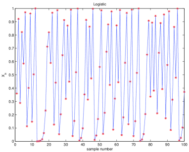
(a) Logistic sequence with $a=4$.

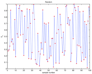
(b) Random sequence.

Figure 1: Random and Logistic sequences.

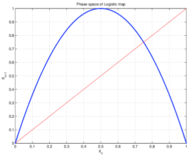
(a) Phase space plot of Logistic sequence with $a=4$.

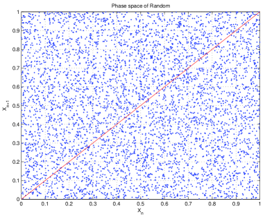
(b) Phase space plot of random sequence.

Figure 2: Phase space plot of random and Logistic sequences.

For simplicity, one-dimensional and two-dimensional chaotic maps are used. More analysis on the Logistic Map is carried out in this paper because it is one of the oldest and typical chaotic maps.

1. One-dimensional chaotic generators:

   Logistic Map[11]

   $$x_{n+1}=ax_{n}(1-x_{n})$$ (2)

   Tent Map[10]

   $$x_{n+1}=\left\{\begin{array}[]{lll}ax_{n}&\mbox{if}\;x_{n}\leq 0.5\\ a(1-x_{n})&\mbox{otherwise}&\end{array}\right.$$ (3)

   Sinusoidal Map[7]

   $$x_{n+1}=ax_{n}^{2}\sin(\pi x_{n})$$ (4)

   Gaussian Map[12]

   $$x_{n+1}=\left\{\begin{array}[]{cll}0&\mbox{if}&x_{n}=0\\ \frac{1}{x_{n}}\;\mbox{mod}\;1&\mbox{if}&x_{n}\neq 0\end{array}\right.$$ (5)

2. Two-dimensional chaotic generators:

   Henon Map[10]

   $$\left\{\begin{array}[]{ll}x_{n+1}=y_{n}+1-a{x_{n}}^{2}\\ y_{n+1}=bx_{n}\end{array}\right.$$ (6)

   Lozi Map[12]

   $$\left\{\begin{array}[]{ll}x_{n+1}=y_{n}+1-a|x_{n}|\\ y_{n+1}=bx_{n}\end{array}\right.$$ (7)

1.3 Switching strategies

Parrondo’s games consist of two games, Game A and Game B. The definitions and rules of each of the games are explained in Section 1.1. At discrete-time step $n$, only one game will be played, either Game A or Game B. The algorithm or pattern used to decide which game to play at discrete-time step $n$ is defined as the switching strategy. In the original Parrondo’s games, the switching strategies carried out are random and periodic switchings.[3] In this paper, chaotic switching of Game A and Game B based on several chaotic sequences is investigated through simulations.

2 Games with chaotic switching

To play Parrondo’s games with chaotic switching, a chosen chaotic generator will be used to generate a sequence, $X$. Sequence $X$ will be used to decide either Game A or B to be played at discrete-time step $n$. There are many ways to carry out this task, but the easiest way is to compare each value of $X$ with a constant $\gamma$. On each round (round $n$) of Parrondo’s games, a value from the chaotic sequence, $x_{n}$ is compared with $\gamma$, if $x_{n}\leq\gamma$, Game A will be played but if $x_{n}>\gamma$, Game B will be played. This simple procedure is adopted in this paper. For random switching, $\gamma$ is equivalent to the proportion of Game A played after $n$ discrete-time steps. However, for chaotic switching, $\gamma$ is not the proportion of Game A played after discrete-time step $n$ unless the chaotic sequence is uniformly distributed.

2.1 Chaotic generators

The outcomes of Parrondo’s games will be affected by the different chaotic switchings applied. Before this aspect is investigated, the parameters that affect the behaviors of the chaotic sequence have to be identified. The properties of a particular chaotic sequence from a chaotic generator depend on two elements: coefficient(s) of the chaotic generator and initial conditions.

2.1.1 Coefficient(s) of a chaotic generator

The phase space of a chaotic signal changes with the coefficient(s) defining its chaotic map as in Eq (2) to Eq (7). That is the relationship between consecutive points of a chaotic sequence changes with the coefficient(s) and this can lead the chaotic sequence to either a chaotic or stable state.[11] For example, the $a$ coefficient in a Logistic Map will decide the state of the sequence generated, whether in a stable or chaotic state. This result can be looked up from the bifurcation diagram of the Logistic map as shown in Figure 3(a). The regions with continuous points correspond to chaotic states, while those with distinct points correspond to stable states.[11] A Logistic sequence with $a=3.74$ is plotted in Figure 4 to show the periodic behavior of the sequence. The bifurcation diagrams of the one-dimensional chaotic maps can be easily plotted as shown in Figure 3(a), Figure 3(b) and Figure 3(c). However, the complete bifurcation diagram of two-dimensional chaotic maps are more complicated since 4 parameters are involved.

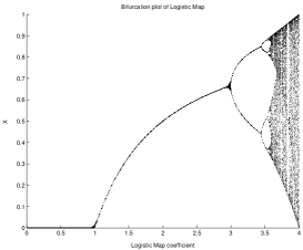
(a) Bifurcation diagram of Logistic Map.

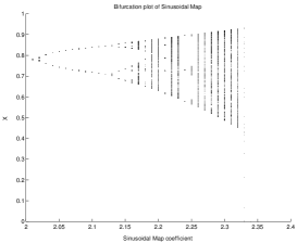
(b) Bifurcation diagram of Sinusoidal Map.

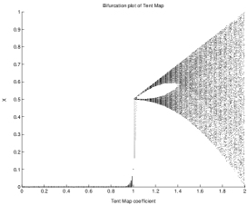
(c) Bifurcation diagram of Tent Map.

Figure 3: Bifurcation diagrams of chaotic maps.

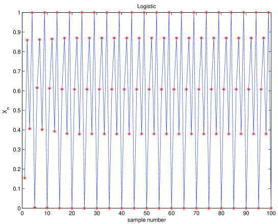
Figure 4: Periodic sequence from Logistic Map with $a=3.74$.

The distribution of $x_{n}$ of a chaotic sequence between 0 and 1 is determined by the coefficients $a$ and $b$ as defined in Eq (2) to Eq (7). With coefficients that correspond to stable states of a chaotic generator, only countable distinct values of $x$ are observed. The pdf of $x_{n}$ for a Logistic sequence in a stable state is plotted as shown in Figure 5(a). In a chaotic state, the spread of $x_{n}$ is more even over the range from 0 to 1. This is shown with a Logistic sequence and $a=4$, in Figure 5(b).

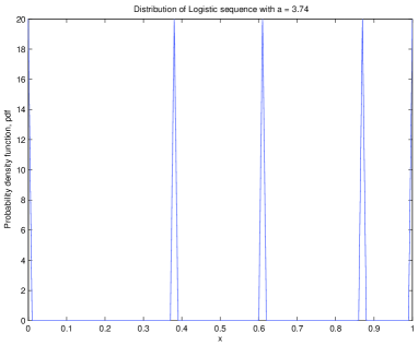
(a) Distribution of Logistic sequence in stable state ($a=3.74$).

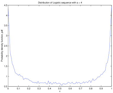
(b) Distribution of Logistic sequence in unstable state ($a=4$).

Figure 5: Distribution of Logistic sequence with different $a$ values.

2.1.2 Initial conditions

Different initial conditions will give the same phase space plot of the chaotic maps. However, initial conditions affect the way the phase space is constructed. A small fluctuation in the initial condition will start a “snow ball” effect on the chaotic sequence, which affects the values of the whole sequence after a few iterations. This is one of the famous properties of a chaotic sequence.[10]

There are some initial conditions that will map the chaotic sequence to a constant value. An example to illustrate this behavior is to use Logistic Map with $a=4$. From simulation results, initial conditions of 0, 1/4, 1/2 and 3/4 will map the sequence to a constant value of either 0 or 3/4. This can be explained from the phase space plot of the Logistic Map as seen in Figure 2(a). The intersections of the phase space plot and the line $x_{n+1}=x_{n}$ occur at $x_{n+1}=x_{n}=0$ and $x_{n+1}=x_{n}=3/4$. These intersection points are the attractors of Logistic Map with $a=4$. The choice of initial conditions in this case drives the sequence directly to the attractors. Hence the choice of initial conditions is vital for obtaining an oscillating sequence in order to carry out effective chaotic switching of Parrondo’s games. Similar attractors can be observed using other chaotic maps.[10]

2.2 $\gamma$ values

To decide whether to play Game A or B, at each discrete-time step $n$, we utilize the $\gamma$ parameter. The $\gamma$ value sets a threshold on selection of games to be played on each round. On the other hand, $\gamma$ value is important to make Parrondo’s paradox appear. The effect of the $\gamma$ value on the rate of winning of Parrondo’s games with chaotic switching is investigated through simulations. All the chaotic sequences are normalized to have values between 0 and 1 for ease of comparison between chaotic switchings with the same $\gamma$ value.

3 Effect of the coefficient(s) of Chaotic generator on the Rate of winning

The rate of winning, $R(n)$, is given below[4], where $\pi_{j}(n)$ is the stationary probability of being in state $j$ at discrete-time step $n$.

$$R(n)=E[J_{n+1}-J_{n}]=E[J_{n+1}]-E[J_{n}]=\sum_{j=-\infty}^{\infty}j[\pi_{j}(n+1)-\pi_{j}(n)].$$ (8)

The coefficient(s) of a chaotic generator will determine the stability of the chaotic system. Under the stable regions, the system will show periodic behaviors. The simulation results show that the maximum rate of winning of Parrondo’s games occurs when the chaotic generator used for switching tends toward periodic behavior. On the other hand, when a chaotic generator behaves truly chaotically, the rate of winning is smaller compared to a periodic case. Hence, under periodic or stable state of a chaotic sequence, and properly tuned initial conditions and $\gamma$ value as discussed in the next section, the rate of winning obtained can be higher than the one achieved by random switching. However, to identify the exact periodic sequence that gives the highest rate of winning is a complicated problem.

For two-dimensional maps such as the Henon Map and Lozi Map, there are two coefficients, $a$ and $b$ that control the behavior of the sequence. Hence, they determine the rate of winning of Parrondo’s games. From Figure 6(a) and Figure 6(b), the gains after 100 games are plotted with different combinations of $a$ and $b$ values. It is found that both the maps give maximum gain after 100 games when $a=1.7$ and $b=0$. For $b=0$, Eq 6 and Eq 7 are simplified to Eq 9 and Eq 10 respectively, which are one-dimensional.

$$x_{n+1}=1-a{x_{n}}^{2},\\$$ (9)

$$x_{n+1}=1-a|x_{n}|.\\$$ (10)

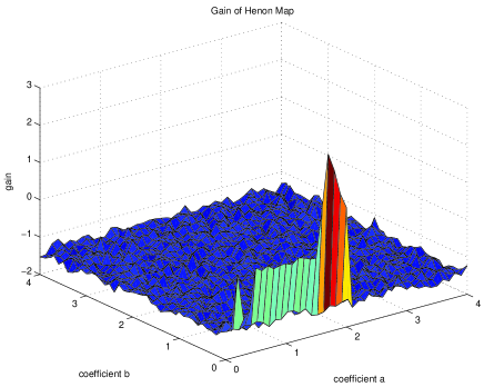
(a) Gain of Henon switching after 100 games with different $a$ & $b$ coefficients.

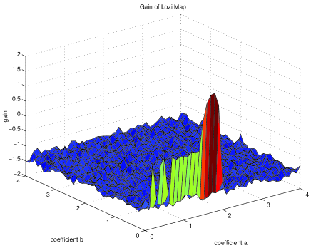
(b) Gain of Lozi switching after 100 games with different $a$ & $b$ coefficients.

Figure 6: Gain of Parrondo’s games with switching based on two-dimensional maps against $a$ and $b$ coefficients.

4 Effect of initial conditions and $\gamma$ value on the rate of winning

Different combinations of the initial conditions and $\gamma$ values give different rates of winning for Parrondo’s game. For some initial conditions, chaotic switching causes the games to lose. This occurs when the initial conditions drive the chaotic sequence towards its attractors as discussed in Section 2.1.2. This situation can be explained as playing Game A or Game B individually since the sequence stays in a constant value. However, the other initial conditions give the same rate of winning for a given particular value of $\gamma$ and coefficient(s) of the chaotic generator. Since the $\gamma$ value decides the proportion of games played, $\gamma$ value can make the games either win or lose, as long as the initial condition is not in the losing region. To obtain optimized or maximum rate of winning, the capital of the games, after 100 games averaged over 5,000 trials against initial conditions and $\gamma$ value is plotted. These 3-dimensional diagrams are shown in Figure 7(a) to Figure 7(d).

For Henon and Lozi Maps, the 3-dimensional diagrams of gain after 100 games against initial conditions and $\gamma$ are plotted using the simplified maps explained in Section 3 in order to obtain maximum rate of winning. They are shown in Figure 7(e) and Figure 7(f).

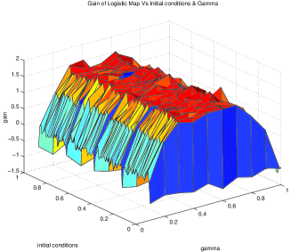
(a) Gain of Logistic switching after 100 games.

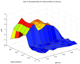
(b) Gain of Sinusoidal Map switching after 100 games.

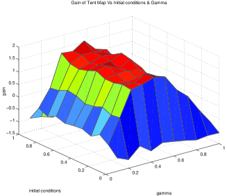
(c) Gain of Tent Map switching after 100 games.

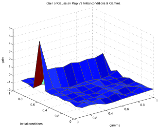
(d) Gain of Gaussian Map switching after 100 games.

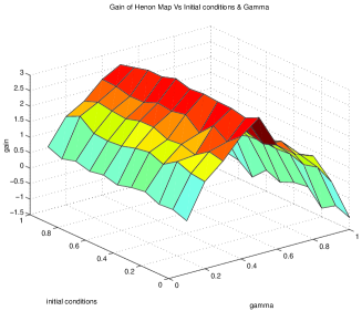
(e) Gain of Henon Map switching after 100 games ($a=1.7$, $b=0$).

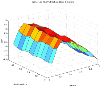
(f) Gain of Lozi Map switching after 100 games ($a=1.7$, $b=0$).

Figure 7: Gain of Parrondo’s games with chaotic switching against initial conditions and $\gamma$ value.

When $\gamma$ and the initial condition are set to 0.5 and 0.1 respectively for a Logistic sequence with $a=3.74$, the maximum gain averaged over 50,000 trials, is found to have value of 6.2 after 100 games.

5 Effect of initial conditions and $\gamma$ value on the proportion of Game A played

The initial conditions of all the chaotic generators have no affect on the proportion of Game A played. However, the proportion of Game A played is significantly dependent on $\gamma$ value. This is because the $\gamma$ value is acting as a threshold value on deciding whether the next game played should be Game A or B. The $\gamma$ value draws the boundary of regions between Game A and B in the normalized time series plot of the chaotic sequence.

6 Comparing different switchings under same proportion of Game A played

The performance of different switchings is based on the rate of winning Parrondo’s games. The higher the rate of winning, the better the performance is. To compare the performance of the switchings in a fair manner, a normalization procedure has to be properly carried out. One suggested way is to compare switchings with the same proportion of Game A and B played. Since the proportion of Game A and B played depends on $\gamma$, $\gamma$ is used to adjust the proportion of Game A played to a certain fixed value (say 0.5) for all the switchings. The graph showing the relationship of proportion of Game A played and $\gamma$ value for chaotic switchings is plotted in Figure 8. The chosen fixed proportion of Game A played for all the chaotic switchings is 0.5, since the proportion of Game A played for periodic sequence of [AABB…] or [2,2], is 0.5. Hence, $\gamma$ is used to obtain 0.5 proportion of Game A played for all the chaotic switchings and random switching. The $\gamma$ value that corresponds to 0.5 proportion of Game A played for respective chaotic switchings can be found in Figure 8 and Table 1. Under this condition, the rates of winning of the games with different switchings can be properly compared. The simulation results of all chaotic switchings discussed together with random and periodic [2,2] switchings are plotted in Figure 9. This shows that Parrondo’s games with chaotic switching can give higher rate of winning compared to one with random switching but may or may not be higher than one with periodic switching. It is found that a particular chaotic switching gives its highest rate of winning when its sequence is periodic with a short period.

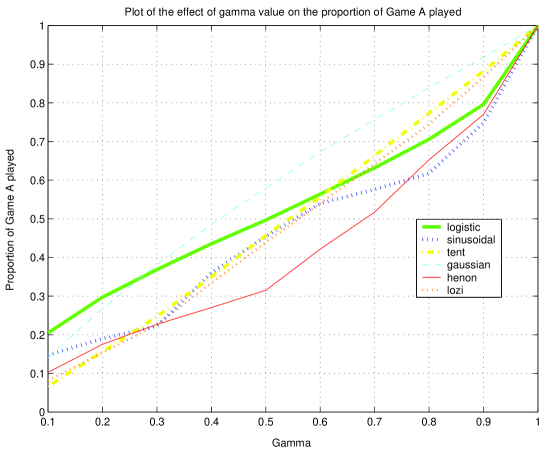
Figure 8: Plot of effect of $\gamma$ on the proportion of Game A played.

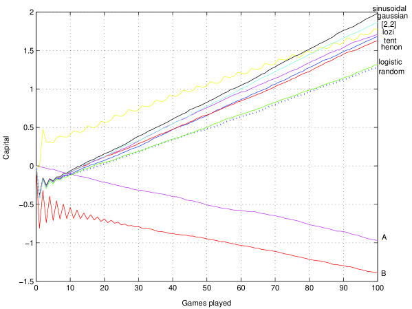
Figure 9: Capital under different switching regimes for 100 games (averaged over 50,000 trials).

7 Conclusion

The proportion of Game A and B played must be equal for all switching strategies in order to compare Parrondo’s games in a fair manner. Parrondo’s games with chaotic switching can give higher rate of winning compared to random switching. The rate of winning obtained from chaotic switching is controlled by the coefficient(s) defining the chaotic generator, initial conditions and proportion of Game A played. When a chaotic switching approaches periodic behavior with a short period, it gives the highest rate of winning on Parrondo’s games. From simulation results, combination of Game A and B in the pattern [ABABB…] is found to give the highest rate of winning.

Table 1: Table showing all the parameter values used in all figures.

Figure	a	b	$\gamma$	Initial condition	No. of trials/
					samples
1(a)	4	-	-	0.1	100 samples
1(b)	-	-	-	-	100 samples
2(a)	4	-	-	0.1	5,000 samples
2(b)	-	-	-	-	5,000 samples
3(a)	0 to 4	-	-	0.1	250 samples
3(b)	2.0 to 2.4	-	-	0.5	250 samples
3(c)	0 to 2	-	-	0.1	250 samples
4	3.74	-	-	0.1	100 samples
5(a)	3.74	-	-	0.1	50,000 samples
5(b)	4	-	-	0.1	50,000 samples
6(a)	0 to 4 step 0.1	0 to 4 step 0.1	0.5	[x,y]=[0,0]	5,000 trials
6(b)	0 to 4 step 0.1	0 to 4 step 0.1	0.5	[x,y]=[0,0]	5,000 trials
7(a)	4	-	0 to 1 step 0.1	0 to 1 step 0.01	5,000 trials
7(b)	2.27	-	0 to 1 step 0.1	0 to 1 step 0.1	5,000 trials
7(c)	1.9	-	0 to 1 step 0.1	0 to 1 step 0.1	5,000 trials
7(d)	-	-	0 to 1 step 0.1	0 to 1 step 0.1	5,000 trials
7(e)	1.7	0	0 to 1 step 0.1	0 to 1 step 0.1	5,000 trials
7(f)	1.7	0	0 to 1 step 0.1	0 to 1 step 0.1	5,000 trials
8	same as below	same as below	0 to 1 step 0.1	same as below	5,000 trials
9	-	-	-	-	-
Logistic	4	-	0.50	0.1	50,000 trials
Sinusoidal	2.27	-	0.55	0.5	50,000 trials
Tent	1.9	-	0.55	0.8	50,000 trials
Gaussian	-	-	0.41	0.701	50,000 trials
Henon	1.7	0	0.68	[x,y]=[0,0]	50,000 trials
Lozi	1.7	0	0.55	[x,y]=[0,0]	50,000 trials