Dissertation
submitted to the
Joint Faculties for Natural Sciences and Mathematics
of the Ruperto Carola University of
Heidelberg, Germany,
for the degree of
Doctor of Natural Sciences
A Modular
and Fault-Tolerant
Data Transport
Framework
presented by
Diplom–Physiker: Timm Morten Steinbeck born in: Aachen
Heidelberg,
Referees: Prof. Dr. Volker Lindenstruth Prof. Dr. Peter Bastian
Ein modulares und fehlertolerantes Daten-Transport Software-Gerüst
Das High Level Trigger (HLT) System des zukünftigen Schwerionen-Experiments ALICE muss seine Eingangsdatenrate von bis zu 25 GB/s zur Ausgabe auf höchstens 1.25 GB/s reduzieren bevor die Daten gespeichert werden. Zur Handhabung dieser Datenraten ist ein großer PC Cluster geplant, der bis zu mehreren tausend Knoten skalieren soll, die über ein schnelles Netzwerk verbunden sind. Für die Software, die auf diesem System eingesetzt werden soll, wurde ein flexibles Software-Gerüst zum Transport der Daten entwickelt, das in dieser Arbeit beschrieben wird. Es besteht aus einer Reihe separater Komponenten, die über eine gemeinsame Schnittstelle verbunden werden können. Auf diese Weise können verschiedene Konfigurationen für das System einfach erstellt werden, die sogar zur Laufzeit geändert werden können. Um ein fehlertolerantes Arbeiten des HLT Systems zu gewährleisten, enthält die Software einen einfachen Reparatur-Mechanismus, der es erlaubt ganze Knoten nach einem Fehler zu ersetzen. Dieser Mechanismus wird in Zukunft unter Ausnutzung der dynamischen Rekonfigurierbarkeit des Systems weiter ausgebaut werden. Zur Verbindung der einzelnen Knoten wird eine Kommunikationsklassenbibliothek benutzt, die von den spezifischen Netzwerkeigenschaften, wie Hardware und Protokoll, abstrahiert. Sie erlaubt es, dass eine Entscheidung für eine bestimmte Technologie erst zu einem späteren Zeitpunkt getroffen werden muss. Die Bibliothek enthält bereits funktionierende Prototypen für das TCP-Protokoll sowie SCI Netzwerkkarten. Erweiterungen können hinzugefügt werden, ohne dass andere Teile des Systems geändert werden müssen. Mit dem Software-Gerüst wurden ausführliche Tests und Messungen durchgeführt. Ihre Ergebnisse sowie aus ihnen gezogene Schlussfolgerungen werden ebenfalls in dieser Arbeit vorgestellt. Messungen zeigen für das System sehr vielversprechende Ergebnisse, die deutlich machen, dass es beim Transport von Daten eine ausreichende Leistung erreicht, um die durch ALICE gestellten Anforderungen zu erfüllen.
A Modular and Fault-Tolerant Data Transport Framework
The High Level Trigger (HLT) of the future ALICE heavy-ion experiment has to reduce its input data rate of up to 25 GB/s to at most 1.25 GB/s for output before the data is written to permanent storage. To cope with these data rates a large PC cluster system is being designed to scale to several 1000 nodes, connected by a fast network. For the software that will run on these nodes a flexible data transport and distribution software framework, described in this thesis, has been developed. The framework consists of a set of separate components, that can be connected via a common interface. This allows to construct different configurations for the HLT, that are even changeable at runtime. To ensure a fault-tolerant operation of the HLT, the framework includes a basic fail-over mechanism that allows to replace whole nodes after a failure. The mechanism will be further expanded in the future, utilizing the runtime reconnection feature of the framework’s component interface. To connect cluster nodes a communication class library is used that abstracts from the actual network technology and protocol used to retain flexibility in the hardware choice. It contains already two working prototype versions for the TCP protocol as well as SCI network adapters. Extensions can be added to the library without modifications to other parts of the framework. Extensive tests and measurements have been performed with the framework. Their results as well as conclusions drawn from them are also presented in this thesis. Performance tests show very promising results for the system, indicating that it can fulfill ALICE’s requirements concerning the data transport.
Chapter 1 Introduction
In high-energy and heavy-ion physics, as in many other scientific and academic applications, compute clusters made up of standard PCs using the Linux operating system have emerged as one of the predominant type of computer systems for data analysis and other tasks requiring large amounts of processing capabilities. The primary reason for this is their very good price vs. performance ratio, owing to the usage of widely available and cheap mass market components. In newest developments, such as the experiments for the future Large Hadron Collider (LHC) at CERN, large clusters will not only be used for offline data analysis but also for online data processing and acquisition. In these types of systems large amounts of data of up to tens of gigabytes per second will be transported through clusters in a data flow fashion, passing through several stages in the processing chain. Due to the flexibility afforded by the building-block like construction of such systems from basically identical components and taking into account the insecurity in the predictions for the future development of that market, a similar flexibility in the software architecture and configuration of these systems is highly desirable. A further prime requirement for these systems is that the transport of the data in a system, both in each node as well as from one node to another, has to be as efficient as possible. The necessity for this requirement arises from the fact that the purpose of these systems is the processing of data from the experiments, for which massive amounts of CPU power are needed. Any CPU cycles used just for transport of the data, without producing any analysis results, increase the total number of CPUs and consequently also PCs in the system needed for the analysis, causing a higher cost. Some overhead for the transport of data is unavoidable but it should obviously be kept to a minimum. Next to the flexibility and efficiency, the reliablity of such a system is a natural third primary requirement. Since the single PCs as elements of a cluster do not possess the reliability necessary for such a system, mainly due to their low cost, a system as a whole must be tolerant with regard to the fault of at least a number of its elements. Also, measures must be taken to ensure that the system either has no parts whose failure disables the whole system, called single points of failure, or that these points consist of especially reliable and thus more expensive components.
This thesis describes a framework that has been developed to be used in the type of online data processing systems described above. It has been designed to consist of a number of independent software components that communicate via a specified interface. They can thus be plugged together as needed to form a data processing chain conforming to the requirements and boundary conditions presented through other characterics of the system, either from detector properties or from the hardware configuration. During the framework’s design and development the focus has been on an architecture and implementation to minimize the processing overhead from the communication of the components and the transfer of the data for a minimum impact on the processing capability of a system as a whole, as described above. Utilizing the dynamic reconfiguration ability inherent in the pluggable component concept together with a number of specialized components, the framework can support setups able to tolerate faults in its software components or hardware parts of nodes as well as even the failures of complete cluster nodes.
The following Chapter 2 provides an overview of computing technology background, helpful in understanding design decisions made for the framework. Also contained in this chapter are a number of sample applications for which the framework can or will be used. Chapter 3 details some of the higher level design decisions and choices made for the framework and gives an architectural overview of it. In the following chapters classes contained in modules of the framework are presented in more detail. Chapter 4 presents utility classes providing basic functionality for the framework. The next chapter describes classes for communication between the nodes in a cluster. These communication classes are based on an abstract interface with implementations available for two different networking technologies and they are used to connect framework components on different nodes. Main parts of the framework, consisting of the interface between the components and a number of components and templates, are detailed in Chapter 6 and 7 respectively. The following chapter 8 presents benchmarks and system tests of the framework and some of its constituent parts, while the final chapter 9 contains the conclusions from the development and tests as well as an outlook for future development possibilities. Additional information for the benchmarks from chapter 8 is contained in appendix A. Tables with results presented in chapter 8 are located in appendix B. Descriptions of a number of developed components which became obsolete later can be found in appendix C. A glossar of frequently used abbreviations can be found in appendix D.
I would like to say many thanks to several people without whom this thesis would not exist as it does:
-
•
My supervisor Volker Lindenstruth for giving me the opportunity to work on this thesis and the HLT project as well as many valuable suggestions, information, and advices.
-
•
My second referee Peter Bastian for his willingness to read and assess my dissertation and take part in my exam.
-
•
Markus Schulz for many informational and fruitful discussions, the good cooperation, as well as his assistance and advice.
-
•
Arne Wiebalck and Heinz Tilsner for much help, discussions, the good cooperation during our common time at the institute, and in particular for proof-reading parts of the thesis.
-
•
The whole group at the Chair for Computer Science in Heidelberg for the comfortable atmosphere and cooperation in the group. It was and is a fun time.
-
•
My parents in general for supporting me during my time of studies and for allowing me to pursue this career, and in particular my father for proof-reading this complete work.
-
•
But most particular and deeply I want to thank my wife Heike for supporting and helping me during the whole time of work on the thesis, especially during the last few months of writing. Without her love, endurance, and support I would not have been able to do this.
Chapter 2 Background
2.1 Computing Background
Overview
Due to the continuously increasing use of clusters made up of commodity PC hardware in high-energy and nuclear physics, for offline as well as for online purposes, the characteristics of this architecture play an increasingly important role in computer architecture for that field. In the following section an overview of the computer technology and architecture in the PC cluster area is given to detail the characteristics and pecularities that influence the design of cluster systems as well as the development of software to be run on them. Emphasis is given to clusters used for scientific tasks, particularly in the use as online data analysis farms for the readout and triggering of high-energy physics experiments, the focus of the software framework described in this thesis. Components of such a system come predominantly from the PC mass market due to the good price-performance ratio present there. On the other hand this necessity for low prices often induces compromises in technology compared to custom solutions, which have to be taken into account when designing a cluster system’s hardware and software.
Introduction to Cluster Technology
Data analysis and other scientific applications have used and relied on computers for a long time and the amount of processing power needed has been rising steadily. Stimulated by recent increases in available computer speed the applications have become more sophisticated, raising in turn the demands for processing power required by those applications. Many of these scientific problems are too large to be handled efficiently by one single processor and thus parallel computers are needed to run these problems efficiently. Prices for most commercially available parallel computers, most of which fall into the high performance computing (HPC) category, are typically rather high for academic budgets. Many institutions have therefore turned to assembling comparatively low cost networks or clusters of workstations [1], [2] (NOWs or COWs) or clusters of PCs, frequently called Beowulfs [3], running Linux [4], [5], [6] or another of the free Unix flavors. These clusters mostly consist of a number of computers made up of commodity-off-the-shelf (COTS) components, and are typically connected either via Fast or GigaBit Ethernet [7],[8],[9],[10],[11],[12] or via a dedicated System-Area-Network (SAN), like the Scalable Coherent Interface (SCI) [13], Myrinet from Myricom [14], or the future ATOLL [15], [16], [17]. These SAN technologies typically have one or more of the following characteristics compared to lower cost technology such as Ethernet: lower communication latencies, higher bandwidth, and smaller processing overhead. The last point can be of particular importance, as more CPU time is available for doing actual processing instead of being used to transfer data.
CPU and Memory Development
The above mentioned COTS components have a very competitive and advantageous price to performance ratio due to their mass market nature. In addition they also allow to take direct advantage of the quickly developing increases in absolute performance in this market. The increases seen here closely follow Moore’s law [18], which in its original form states that the density of circuits on chips will increase by a factor of 2 every year. Derived forms state that the same behavior, with different factors, applies not only to the density but also to the performance of the chips. The most visible aspects for mass market PCs are the increase in CPU clock frequency, which by now roughly doubles every 18 months, as well as the increase in memory size.
The usage of mass market components however has some disadvantages as well. While processor performance and memory size closely follow Moore’s law and thus increase by 60 % every year, the memory access time only increases by 2 % per year. Special purpose high-performance computing hardware can implement more elaborate measures to work around this problem than commodity hardware, as the latter is typically optimized for a low cost. This causes the gap between raw processor performance and the speed of accessing data in memory to widen every year [19]. As a result it is increasingly costly when a processor cannot access data in its cache but has to load it from memory. The processor has to perform several wait cycles, during which it cannot perform any processing. The cost of memory access is most obvious in applications that access large memory blocks in irregular patterns, which mitigates the utility of caches.
Busses and Networks
A similar situation arises concerning extension busses and network interfaces. The bandwidth and latency of these parts also have been unable to keep up with the advances in CPU speed. In the bus area the Peripheral Component Interconnect (PCI) bus [20], [21] with 64 bit and 66 MHz has only become established in the high end PC server/workstation market. PCI-X with up to 133 MHz is just starting to appear there. The bandwidth of the 64 bit/66 MHz version of this bus reaches a theoretical peak performance of 528 MB/s, with the slower 64 bit/33 MHz and 32 bit/33 MHz versions reaching 264 MB/s and 132 MB/s respectively. Even though the 64 bit/66 MHz bus has a factor of 4 advantage over the 32 bit/33 MHz version still dominant in the home PC segment, its peak performance is still at least a factor of 4 lower compared to contemporary memory interfaces. The current predominant network technology in the PC market is 100 Mb/s Fast Ethernet with Gigabit Ethernet establishing itself especially for servers. In cluster systems SANs are used for interconnects as well, sometimes coupled with proprietary network protocols. But as these technologies can be several orders of magnitude more expensive compared to Ethernet, especially the 100 Mb/s variety, many clusters are constructed using the more cost-effective interface choice. The communication protocol used on these Ethernet adapters is practically always the standard Internet TCP/IP protocol suite [22]. This network protocol/interface combination has the advantage of being widely available, cheap, and reliable. However, neither of its parts was designed for the task of a cluster interconnect or SAN. Next to the obvious disadvantages of relatively low bandwidth and high latency, this combination is not the optimal solution for this task because of another drawback. The TCP/IP protocol consists of a protocol stack with several layers of protocols inside the operating system kernel. Data sent from a user application first has to be copied from the user level memory into the privileged kernel space (or system) memory. It then passes through the protocol layers where the data is often copied from layer to layer. These copy stages have to be done by the computer’s CPU, preventing it from executing actual processing tasks. Additionally the CPU needs to access memory twice (read and write) to copy the data. These memory accesses first slow the CPU down as it now has to wait for the memory while copying and second they take up much of the already precious memory bandwidth in the system. For systems sending large amounts of data this can have a quite detrimental effect on other applications running at the same time. These influences are due to several factors: the memory bandwidth being used by copying processes, the filling up of cache space with the copied data, and the pure CPU usage itself. But even on better TCP/IP implementations where the data is not copied between the layers, the first copy stage is practically always present, and the protocol stages with their required processing have to be passed as well. So in addition to being a comparatively slow network, both as far as latency and bandwidth are concerned, coupled with the most widely used protocol Ethernet also uses up more precious system resources than other technologies for connecting clusters. A rule of thumb is that for every Megabyte of data transferred per second with TCP/IP over Ethernet depending on block size at least 1 % CPU usage is incurred.
Commodity-Off-The-Shelf and High-Performance-Computing Hardware
As the COTS market relies on interoperability of its components, especially in the area of memory and extension busses with their respective add-on cards, the technological advances in this area and the market acceptance are comparably slow. HPC system vendors on the other hand, have no such compatibility constraints and are free to use tailored and tuned interfaces and components in their systems. These special purpose components give them a performance advantage compared to the cheaper clusters and earn them the classification of high performance computers. Despite these technological and economical differences a lot of recent HPC and cluster-type systems share a principal similarity. Both are composed of relatively cheap and standardized building blocks connected by a network. But whereas for clusters the nodes are single PCs, sometimes even dual CPU PCs, HPC systems are often composed of Symmetric Multi Processor (SMP) systems, sometimes with more than 100 CPUs. Similiarly, where most clusters are connected via Fast or Gigabit Ethernet and some with specialized SANs, many HPC systems feature specially developed interconnects between the nodes with bandwidths comparable to the internal busses in PCs.
Comparing the price/performance ratio of typical clusters and HPC systems for a single CPU, clusters rank much better than their more expensive counter-part. For easily parallelized problems which feature a high ratio of computation on each node to communication between the nodes, a cluster offers much better overall performance for the same price or a comparable performance for a much lower price. Most problems in high-energy and nuclear physics are of that type and are thus well suited for clusters.
Cluster Software
On the software side the widespread use of clusters has been primarily made possible by the rise in popularity and support of the Linux (or GNU/Linux) [4] operating system. This clone of the Unix operating system, freely available in source code, has begun its life on PC systems and is now available for a wide range of hardware. Due to its popularity a wide spectrum of PC hardware extensions, e.g. network adapters or graphics cards, is supported with drivers. Also due to its widespread use coupled with the source code availability many people have been able to search for errors in it. As a result bugs are usually found quickly and Linux thus has a reputation as a very stable and reliable system. Since the scientific and especially the academic area has for a long time been involved with Unix and has been using it widely, Linux has enjoyed an especially quick acceptance in this area. Coupled with other software freely available in source code, and thus adaptable, it has established itself as a well suited operating system companion for cost-effective clusters made up of PC components. Recently other free Unix like systems, e.g. FreeBSD [23] or OpenBSD [24], some of them actually older than Linux, have also gained popularity, but Linux was the starting point for cheap Unix like cluster systems and is still the most widespread operating system there.
Motivated by the increase in cluster usage a number of software packages have been developed to ease the administration of a cluster. Most of these packages follow the principle of allowing the administration of the cluster as a single system and not as a collection of systems. The most extreme of these systems like Mosix [25], [26], [27] and its derivative openMosix [28] treat the whole cluster as a single system by allowing process migration over a network between the nodes for a cluster-wide load-balancing. Other systems support the creation of batch-queue systems for separate jobs, to be dispatched to available cluster nodes for processing, or monitor the cluster nodes from a central location. Examples of such packages are the open source Compaq [29] (now Hewlett-Packard (HP) [30]) Single System Image (SSI) Clusters (SSIC) package [31], the Load Sharing Facility (LSF) [32] from Platform Computing [33], and the Condor package [34], [35], [36].
A number of packages also exist for communication inside a cluster. The most well-known of these are the two Message Passing Interface (MPI) [37], [38], [39], [40] implementations MPICH [41] and LAM/MPI [42] and the Parallel Virtual Machine (PVM) [43]. These three packages are designed for parallel applications that run distributed on multiple PCs and frequently exchange data with each other. Data exchanges are primarily done between iterative calculations, processed data is sent to other processes and received data is used as the basis for new calculations. These packages therefore are typically not optimized for an efficient communication but rather one with a low latency. Fault tolerance also is not one of the prime foci of these packages, as calculations can easily be restarted with the same input data.
Interfaces to Readout Hardware
Another important segment for computers in sciences is the readout of data from experiment setups. For a long time computers in this area have been equipped with the busses used for the connection of instruments, e.g. VMEbus [44], [45], [46] or CAMAC [47], [48]. These computers are typically based on CPUs used in the desktop market, e.g. Intel x86 or PowerPC, and often run real-time operating system like VxWorks [49] or LynxOS [50]. Both hardware and software are very specialized and as a result have a small market, making them relatively expensive compared to common desktop hardware and operating systems. For this reason, a trend similar to the cluster tendency for parallel computing has set in to replace these special systems with standard PCs as well. Where instrument connections are needed interface cards for PC busses (mostly PCI) provide the necessary connections to other equipment. In other cases special hardware is being developed to interface experiment equipment with read-out computers with PCI or another of the PC system standard busses on the computer side. Despite its age and comparably low performance the old Industry Standard Architecure (ISA) bus introduced with the first IBM PCs still enjoys some popularity here, especially in industry applications. But for new developments in the scientific area PCI is now very often used, enabling the use of COTS systems for readout as well as for calculation.
As these special hardware readout devices have to be accessed and are in general not supported by operating systems due to their custom nature, specific software for them has to be provided as well. Development of device drivers for them is often too complicated and due to the frequently required rapid development not feasible as well. Therefore mostly normal programs are used that require some special features or privileges to gain direct access to the readout hardware. To faciliate the development of these programs, packages or drivers exist that provide generic and easy access to any hardware in a system. With this principle, development of a driver is required only once. It can be utilized in user-space programs afterwards.
2.2 Applications for a Data Transport Framework
2.2.1 High-Energy and Heavy-Ion Physics Experiment Trigger Systems
A major area of application for a data flow framework are readout and especially trigger systems for experiments in high-energy and heavy-ion physics, as these are inherently of a data driven nature. Data arrives in chunks, the detector’s events, which have to be processed. Often one event arrives in multiple parts, which have to be assembled before, after, or as a part of processing. Depending on the exact nature of the experiment the analysis might have to be executed in a number of steps. Each step requires the data from previous ones, mostly the directly preceeding. Data is thus passed or flows from station to station, possibly being merged with data from other stations, until the desired result is obtained or it is written to permanent storage. Due to the high rates required most often in the lower levels of such trigger systems, a relatively generic software framework is not very well suited there. Instead more specialized software or even hardware is required for these levels.
Concerning the upper level trigger systems very high data rate requirements are currently found in the new generation of (relativistic) heavy-ion physics experiments. With their high occupancies, the resulting large event sizes coupled with still considerable event rates of at least several hundred Hertz, and consequently very high data rates, they present one of the biggest challenges in online data processing for PC clusters. Among these one of the most advanced is the ALICE experiment planned for the heavy-ion running mode of the future Large Hadron Collider (LHC) at CERN in Geneva. Two other projects, not progressed as far as ALICE, are the future Compressed-Baryonic-Matter (CBM) and Proton-ANtiproton-at-DArmstadt (PANDA) projects at the Gesellschaft für Schwerionenforschung (GSI) in Darmstadt.
2.2.2 The ALICE Detector and the ALICE High Level Trigger
The ALICE Detector and the Quark-Gluon-Plasma
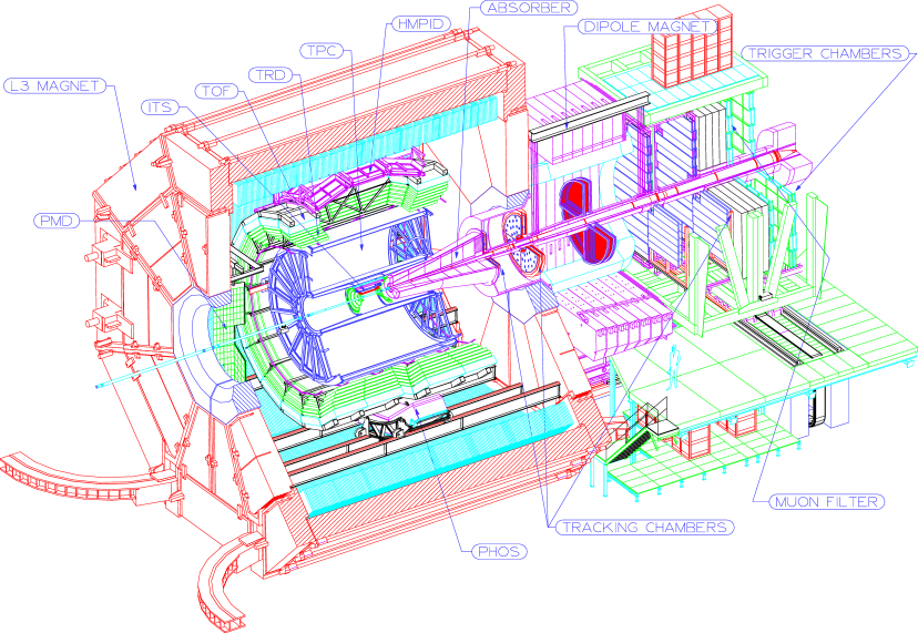
The primary application for which the framework has been developed is the ALICE experiment’s [51], [52], [53], [54] last trigger stage, the High Level Trigger (HLT). ALICE, shown in Fig. 2.1, is a detector for relativistic heavy-ion collisions currently being developed and built for the future Large Hadron Collider (LHC) [55] at CERN [56]. The LHC will be operated in two modes: proton-proton (pp) mode and heavy-ion (HI) mode. In the primary proton-proton mode LHC will collide bunches of protons every 25 ns corresponding to a collision rate of 40 MHz. In heavy-ion mode bunches of lead or calcium nuclei will collide every 100 ns or at 10 MHz respectively. ALICE will operate both in pp and HI mode although the detector is primarily designed for heavy-ions, where its main purposes are the search for and investigation of quark-gluon-plasma (QGP). QGP is a new state of matter in which quarks and gluons can move freely in a volume and are not subject to the usual confinement for strongly interacting particles. Overviews of QGP can be found in [57] to [62]. The temperature or energy density in the corresponding volume has to be high enough to enable this state to be established. The minimum required energy density is predicted to be around , roughly 7 times the density of normal nuclear matter. Comparable energy densities have existed during the first few microseconds after the Big Bang. It is expected that by colliding highly energetic lead nucleons it will be possible to reproduce conditions which feature high enough energy densities to allow the formation of quark-gluon-plasma. When the highly energetic fireball produced by the collision expands, it simultaneously cools down and the energy density decreases again. The quarks and gluons in the plasma then have to recombine again to hadrons undergoing the normal color confinement. From these hadrons and additionally produced leptons observed in the detector, one has to extract information about the system that existed during the collision. The number of particles produced in these collisions is very large. For ALICE of the order of particles are expected for a collision in the covered pseudo-rapidity range of . The minimum bias collision rate at the LHC heavy-ion design luminosity of is several 10 kHz. Combining event rate and particle multiplicity leads to a very high amount of data produced. Together with the preceeding trigger stages the HLT’s task is to reduce that data volume to a rate more manageable for mass storage and also to make the most efficient use of the available output bandwidth by storing only the most interesting events and compressing each event’s data to reduce its size.
ALICE’s Subdetectors
The detector consists of a number of sub-detectors, most of them arranged in a layered shell structure around the beam pipe covering a solid angle of almost and a pseudorapidity range of . Closest to the beam pipe is the Inner Tracking System (ITS) [63], whose primary purpose is the detection and reconstruction of the primary and secondary vertices and track-finding for charged particles with a low transversal momentum that do not enter the Time Projection Chamber (TPC) (see below). In addition it will also be used to improve the momentum resolution of particles with high momentum as well as for the reconstruction of low energy particles and their identification. Six cylindrical layers of detectors make up the ITS with a high enough space point resolution to cope with the expected high particle densities. The layers will be placed at radii from 3.9 cm to 45 cm and will extend from the interaction point (IP) where the collisions occur in both directions along the beam pipe. They extend from 12.25 cm for the innermost layer to 50.4 cm for the outermost one. For the two innermost layers, where the particle tracks are most dense, silicon pixel detectors (SPDs) have been chosen as they provide the best possible granularity and resolution at these small radii. Furthermore, they can be operated at high rates and will be used to determine an event’s vertex together with the muon spectrometer. The two middle layers have a lower track density due to their larger distance from the IP. Silicon drift detectors (SDDs) are used here as they are cheaper than SPDs and have the ability to provide additional information for particle identification. In the two outermost layers silicon strip detectors (SSDs) are sufficient to satisfy the less severe resolution requirements and the comparatively large area here makes it desirable to use this proven, reliable, and especially cheaper technology.
Outside of the ITS is the Time Projection Chamber (TPC) [64], [65], [66], [67], both ALICE’s physically largest sub-detector as well as the one producing the largest amount of data. It is the primary detector used for track finding and momentum measurements as well as for identification of particles by their specific energy loss . The TPC is a cylinder around the beam pipe measuring 5 m in length with a central high voltage plane. Its inner and outer radii are 88 cm and 2.5 m respectively. At the endcaps are readout chambers consisting of Multi Wire Proportional Chambers (MWPCs) to amplify and read out the signals of the particle tracks. Most of the TPC’s characteristics are results of the expected high particle multiplicity and the resulting problems of distinguishing separate particle tracks. Its inner radius has been chosen so that the expected particle density on the inner surface is around . For the outer radius the criterion was to obtain a length of tracks inside the TPC that will allow a measurement with a precision of 6 - 7 %. The length finally is determined by ALICE’s design coverage of with a drifttime chosen to be . Due to the high particle multiplicity a very fine granularity of pixels has been chosen to achieve a good two track separation ability. This fine granularity is the reason why the data volume produced by the TPC is the largest part in ALICE. Expected event sizes for the TPC, already zero-suppressed and runlength encoded, are about 60 - 70 MB for central HI events. The readout chambers are arranged in 159 pad-rows in each slice, with pad sizes of , , and .
Directly adjacent around the TPC and primarily designed to complement its electron identification capability is the Transition Radiation Detector (TRD) [68], [69]. Its primary purpose is to provide electron identification capabilities for the central barrel region for momenta beyond . Additionally, the TRD should enable a thorough research of the dilepton continuum found in the central barrel region. As the TRD is a fast detector and especially a fast tracker it also contributes an effective triggering capability for particles, particularly electrons, with a high transverse momentum (). Another trigger type of the TRD is the selection of hadronic jets with a high transversal energy. With the tracking information being available a few microseconds after each event, it becomes possible to select events with high particles and activate the TPC’s gating grid for readout only for those events. To optimally cooperate with the TPC the TRD has been designed to have the same acceptance of . It consists of six layers of chambers between radii of 2.9 m and 3.7 m. Each layer is divided into five segments along the beam axis and 18 segments around the detectors circumference. The total number of chambers is thus 540 with each chamber consisting of a combination of foil stacks to produce transition photons, Xenon filled MWPCs to detect them, and front end electronics for readout. A chamber uses between 12 and 16 pad rows in the direction of the beam axis and each pad row consists of about 144 pads read out. The total number of channels in the TRD is about , making the TRD the second largest producer of data among the ALICE detectors.
Outside of the TRD is a large Time-Of-Flight (TOF) array dedicated to provide particle identification information for particles of average momentum [70]. It is designed to have a large acceptance and covers a barrel area of about . Momentum coverage for hadrons is between about and . is the upper limit for which the TPC is still able to separate Kaons and Pions based on its information and is the limit for sufficient particle statistics in single event analysis. The overall timing resolution of the system is designed to be around 100 ps, which would allow separation of Kaons and Pions up to momentum. For electrons the momentum range to be covered is between and , where information is not sufficient to distinguish electrons and pions. In this application the timing resolution is of a lesser significance. As the overall inefficiency of the TOF is to be below 20 %, the occupancy of the detector is required to be less than 10 % at the highest particle multiplicities expected, resulting in more than channels being used in the TOF. The baseline technology choice for the TOF are Pestov spark counters, which have a number of advantageous features. Foremost among these is their very good time resolution reaching up to 25 ps. In addition they feature a lifetime corresponding to a running time of more than 20 years as well as an intrinsic efficiency of more than 96 % and do not require preamplifiers due to their high signal output. Major drawbacks, however, are a lack of experience with systems on a similarly large scale and a time comparable to the projected operation of ALICE. Therefore a fallback solution of Parallel Plate Counters (PPCs) is intended, an established technology that would have a lower resolution but would still fulfill the requirements from the physics goals.
Complementing the identification capabilities for particles outside of the momentum range covered by the TOF is the High Momentum Particle Identification (HMPID) detector [70], a Ring Image Čerenkov (or Cherenkov) Counter (RICH). Its area is small compared to the TOF, only and it is placed at the top of the detector at a radius of 4.7 m where the particle density is low. As the particle density of and event rate of around 10 kHz expected to be encountered are nonetheless still high for a detector of this type, a fast-RICH layout implementation is used. Another advantage of this technology is the ability to operate at much higher rates than the ones intended for heavy-ion operations at the LHC so that it can be used in pp-mode as well. The drawback of this techology is a cathode segmented into many small pads which requires a pixel like readout with highly integrated electronics and a large number of readout channels.
Located opposite of the HMPID on the bottom side of the detector is the Photon Spectrometer (PHOS) [71] whose primary purpose is the search for direct photons produced during heavy-ion collisions, which reflect to a high degree the initial conditions found in these collisions. As a secondary task the PHOS also has to measure the production of the neutral mesons and , for which the momentum resolution at is approximately an order of magnitude better than what the tracking detectors can achieve for charged particles. Unfortunately, there is a large background of photons being produced in decays of hadrons with a ratio of direct to decay photons of approximately 5 %. Due to the required detector sensitivity of about 5 % it becomes necessary to measure the rates and transversal momentum spectra of photons as well as and mesons in the same detector. The resulting very high multiplicity in turn necessitates a fine segmentation of the calorimeter, a large distance from the vertex, and a material with a small Molière radius to reduce the transversal extension of the produced showers. To achieve the intended particle occupancy of less than 3 % in heavy-ion collisions at a radius of 4.6 m has been chosen as the material for the PHOS because of its Molière radius of about 2 cm. In order to prevent charged hadrons from producing unwanted signals in the PHOS, a veto-detector will have to be placed in front of the PHOS to reject them. Similarly a system of applying time-of-flight cuts is considered to suppress the signals from neutral hadrons other than and .
One of the most promising signatures for the production of the quark-gluon-plasma is the suppression of the heavy quarkonium resonances, whose decays can be well detected by muon-pair production. To distinguish the signature for QGP from other processes that could also cause this suppresion, it becomes necessary to measure the relative suppression of the different states as well as the ratios to unsuppressed reference processes such as the inclusive heavy quark production. In addition the suppression has to be measured as a function of the transversal momentum spectrum down to its low regions. The search for the produced muon pairs will be done only in the forward direction of ALICE, along the beam pipe, and outside of the normal barrel construction for a number of reasons. Because of the shielding required for the background photons and hadrons only muons with a momentum of at least can be detected and the muons in forward direction will have a higher momentum due to Lorentz-boosting. The pion and kaon background is also reduced in that direction due to the higher momenta required to penetrate the absorbers and the generally lower particle multiplicity per rapidity unit.
The first part of the dimuon arm [72], [73], [74], [75] after the detector barrel are the absorbers already described. They are needed to reduce the particle background consisting especially of photons and hadrons coming from the vertex to acceptable levels, resulting in the momentum cut for muons at . But even with the absorbers in place the main problem for the dimuon arm is still the particle multiplicity in each event rather than the event rate. To cope with this problem the tracking system after the absorbers uses a high granularity so that the maximum expected occupancy is around 5 %. The tracking system is made up of five stations consisting of two chamber planes per station. Each chamber plate in turn has two cathode planes read out to provide two dimensional track information. Intermixed with the tracking stations is a large dipole magnet, with two stations each in front and behind it and one inside the magnet. After the fifth tracking station is another passive muon filter wall in front of four planes of Resistive Plate Chambers (RPCs) as muon identification and trigger detectors. The RPCs are arranged in two stations, each one providing and coordinates. Coordinate differences of the two chambers are used to determine the muons’ transversal momentum for the trigger decision. The whole muon arm covers an angle range from 2° to 9°, a compromise between detector acceptance and cost. It is shielded from the beam pipe by an inner shield for protection from particles produced at large rapidities.
One of the pieces of information needed to determine the collision types that occured is the impact parameter of a collision, a measure for the distance between the centers of colliding nuclei. The observable allowing the best conclusion to the actual impact parameter is the energy carried away by spectator nucleons from the beam that did not take part in the collision. Spectator neutrons and protons have a different charge to mass ratio compared to the ions in the beam. Therefore they will be separated from the beam by the same LHC dipole magnet that also separates the two colliding beams after the interaction point. Detection of the spectator nucleons will be done in two Zero Degree Calorimeters (ZDCs) [76] on each side of the interaction point at a distance of 92 m. Each of the two neutron calorimeters (ZN) will be placed between two beam pipes and will have to fit in the free space between them. The ZN transversal dimensions are therefore restricted by this free space and have been set at . Their depth of corresponds to 10 interaction lengths of the chosen shower material, which must have a high density to place enough absorption capability in the restricted space. By contrast the two proton calorimeters (ZP) are placed to the side of one of the beam pipes and do not suffer from such tight space restrictions. Less denser and cheaper materials can be used in them and the dimensions selected here are , the chosen depth also corresponding to . Quartz fibres have been chosen as the active material both for ZN and ZP in which shower particles produce Čerenkov light read out by photo-multipliers. The primary reason why quartz will be used instead of conventional scintillators is its radiation hardness. In addition, it also provides a good energy resolution even with small calorimeters, like the ZN, and is insensitive to radioactive background whose particles do not produce Čerenkov light. Nonetheless to avoid unnecessary radiation exposure that might damage them, the ZDCs will be removed from the beam pipe during proton-proton mode, when their operation is not required
Another detector covering the forward direction outside of the barrel is the Forward Multiplicity Detector (FMD) [76], measuring the distribution of particles per unit of pseudo-rapidity outside the central acceptance region of the barrel detectors. Additionally, it will provide information for the Level 0 (L0) and Level 1 (L1) triggers (see below) after an event as early as possible. Currently two possible choices exist for the FMD, either Micro Channel Plate (MCP) or Silicon multipad detectors. To determine the multiplicity in a pp event using the MCP one would simply read out and count the number of digital hits, while in heavy-ion mode it would be necessary to sum up the analogue information of the charge collected on each of the anode pads. MCPs have the advantage of very good timing properties with a resolution of about 50 ps. With this resolution MCPs could provide multiple types of information for the TOF and trigger systems, like event time , a first z-coordinate measurement of the event vertex, identification of beam-gas reactions, as well as a measure of pile-up protection for slower detectors, like the TPC. By contrast, the Si multi-pad detectors feature a time resolution of about 20 ns to 40 ns compared to less than 100 ps required. Advantageous for the Si detectors is the fact that they are well suited to multiplicity measurements in heavy-ion collisions and are often used for that purpose already. One possible approach therefore is the use of a combination of MCP and Si detectors. The FMD consists of seven disks arranged around the beam pipe at distances from the vertex from 42 cm to 225 cm. Inner radii of the disks range from 42 cm to 80 cm and outer ones from 105 cm to 175 cm. Together the disks cover the pseudo-rapidity ranges of 1.6 to 3.6 on the side where the muon arm is located and 1.4 to 4.7 on the opposite side. Each of the disks will be divided into several pad segments with the total number of pads on all seven disk being about 780. Due to the analogue summation for the MCPs and the general Si characteristics it will not be necessary to have a high granularity to cope with the high multiplicity.
Contrary to most other detectors ALICE does not feature any large calorimeter detector in the central barrel region. Due to the large radii that the tracking detectors need to handle the high particle multiplicities, any such calorimeter would have to cover a very large surface and be very expensive as a result. Instead ALICE relies on multiplicity measurements of charged particles which on average show a good correlation with the transversal energies in events. To provide some additional information about the transversal energies the Photon Multiplicity Detector (PMD) [76] has been added to ALICE. The PMD is a preshower detector that distinguishes photons from charged particles, especially hadrons, and measures the energy depositions of transversing particles. While the energies deposited by individiual photons show large fluctuations, these are considerably reduced when the depositions of a large number of particles are added for each event. In this way the PMD takes advantage of the high multiplicities that present a problem for most of the other detectors. The forward region was chosen for the PMD as the photon energies are higher in that direction, again due to the rapidity boost, and the area that needs to be covered is comparably small and manageable. It will be mounted on the door of the L3 magnet (see below) at a distance of 5.8 m from the vertex and covers the pseudo-rapiditiy range .
For the magnetic field ALICE will reuse the magnet [77] of the L3 detector [78], [79], [80]. This detector will have been dismantled by the time the LHC will start to operate and ALICE will actually be assembled and operated in the same underground cavern as L3. The magnet’s coil has an inner radius of 5390 mm while the yoke’s outer radius reaches 7900 mm and its length 14100 mm and the magnet’s total weight is about 7800 t. 168 separate octagonal turns make up the solenoidal coil, each with a conducting section of . At the intended magnetic field strength of 0.6 T the magnet will draw several Megawatt of electrical power. After its operation in the L3 detector concerns exist about its continued operation in ALICE, primarily regarding the magnet’s cooling system. Investigations of the current state are in progress and a number of possible modifications for the cooling systems are already under discussion to assure the magnet’s continued functioning during ALICE’s operation.
The ALICE Trigger System
One major problem of high enery and nuclear physics experiments is that the different types of events as well as the respective underlying physical processes occur statistically distributed. Processes with a higher probability therefore produce events more often than rarer processes and are better researched and understood already. As a result rare events are of much more interest to current experiments like ALICE. To increase the number of events available for analysis, trigger systems are used to select events indicated by certain signatures to belong to interesting rare processes. ALICE’s trigger system [81] before the HLT is made up of three stages: Trigger Level 0 (L0), Level 1 (L1) and Level 2 (L2). The system will be active both in pp as well as in HI mode. The primary objective of ALICE is the study of the hot dense matter created during central collisions of heavy-ions. Correspondingly the main emphasis of the trigger system’s design has been on these collisions of ions with relatively small impact parameters. The impact parameter can be determined to a given extent from the particle multiplicity in the FMD and the energy deposited in the ZDC. As central collisions occur relatively frequently the trigger does not need to be very selective and the most common event types can even be scaled down so that only a subset of them is processed.
Dimuon events with particles in the mass range to be observed on the other hand occur very rarely and are therefore processed with a high priority. The first trigger for these events signals that two particle tracks above a specific momentum threshold have reached the dimuon RPC trigger chambers. For these events it is desirable to read out the full data to perform correlations with other observables. In case of pile-up for a dimuon event it will be tried to read a reduced subset of detectors with usable event data. Readout time for such a subset will be about compared to about 2 ms for a full set of detectors.
The purpose of the first trigger stage L0 is to signal an event as soon as possible after occurance using exclusively data from the FMD. The latency of this signal is fixed to . To verify that an event occured three items are checked:
-
•
Whether the interaction point reported is close to the nominal collision point.
-
•
Whether the forward/backward distribution of particles in both directions of the beam pipe is consistent with a beam collision.
-
•
Whether the multiplicity reported from the FMD is above a given threshold.
To prevent non-central events with a muon pair being discarded at this stage the L0’s requirements on centrality are not very strict. A positive L0 signal is used by some of the detectors, amongst them the RICH and the PHOS, to strobe their front end electronics for readout.
The L1 trigger’s decision latency time is fixed to [69] after an event has taken place. Its decision is based on FMD and ZDC information about the centrality of the event, TRD data about high momentum electrons and information from the dimuon system. Since more complex correlations have to be examined for the dimuon system its data is only available at this stage. Any event for which the dimuon trigger reports two particles with a high transversal momentum is then classified as a priority event. An L1 accept signal is issued in that case to all detectors, in order to activate the readout of all detectors’ front end electronics. For the TPC the gating grid is activated, its maximum gating rate is 200 Hz for HI and 1 kHz for pp mode.
After the gating has been activated, the drifttime of has to pass before the TPC can be read out. During this time further processing of data already available from fast detectors can be performed in the L2 trigger stage. Among the possibilties for processing are a mass cut on the dimuon system or fast analysis of data from the FMD. Unlike the first two stages L2 does not have a fixed latency but an upper bound as defined by the drifttime given above. Due to the variable latency the decisions cannot be synchronous anymore. After a positive L2 decision the data from all detectors’ Front End Electronics (FEE) will be read out.
Another part of ALICE’s trigger is a past-future protection system keeping track of pile-ups of overlapping events in each sub-detector. Readout of data is then restricted by the system to a subset of detectors with non-piled-up data. Using the output of the past-future protection unit, an identifier describing the class of event that occured is generated. This is distributed to each of the sub-detectors which then decide what to do with their data for this event.
The Data Acquisition System in ALICE
As the trigger system the Data Acquisition system (DAQ) of ALICE, DATE, [82], [83], [84] will have to run both in proton-proton as well as in heavy-ion mode. As the data rate in pp-mode will be only one fifth of what is expected for HI the main requirements on the DAQ system are given by heavy-ion operation, although this will only be active for a few weeks every year. In general the DAQ system will have to cope with two types of events in this mode. The first will contribute most of the total data stream and consists of central events at a relatively low rate but with a large event size. In contrast, the second type of events contains a muon pair that has been reported by the trigger and is read out with a reduced detector subset, including the dimuon arm. Events of this type can occur at a rate of up to 1 kHz. These two requirements of a large data stream and a rather high event rate will both have to be handled by the DAQ system. In summary the system will have to cope with an aggregate data stream to the permanent data storage (PDS) of 1.25 GB/s.
The Architecture of the system is based on PCs connected by TCP over Gigabit Ethernet. Local Data Concentrator nodes (LDCs) are connected to the detector Front End Electronics (FEE) via optical links, the Detector Data Links (DDL). Each DDL link ends in a PCI Read-Out Receiver Card (RORC) located inside an LDC. One or more RORCs can be placed into each LDC and data from each sub-detector may be read out over several DDLs so that data from one event can be scattered over multiple RORCs and LDCs. Subevent data read out from the detectors in the LDCs is sent to Global Data Concentrator nodes (GDCs) for global event building. A GDC destination for a particular event is determined by the Event Destination Manager (EDM) which communicates this decision to the LDCs. Fully assembled events are shipped to permanent storage for archiving and later offline analysis.
The ALICE High Level Trigger
Together with the preceeding trigger stages the task of the High Level Trigger (HLT) [85], [86] is to maximize the physics output that can be attained by ALICE with the specified bandwidth to tape. To achieve this goal two approaches of online filtering and analysis are possible, which may also be used in combination. The first approach is the customary selection of the most interesting events as described already for the other trigger stages. In the HLT this selection will be performed by an online analysis of events to determine the amount and type of particles that passed through the detector. Among the detectors whose data will be analysed at this time are the ITS, TPC, TRD, and dimuon arm. The second possibility is to compress the events so that a greater number of them can be written to tape. Best compression results are achieved by this approach if the compression method used is adapted to the underlying data. This is similar to the approach taken for MP3 [87], [88] or Ogg Vorbis [89] audio files, where the results achieved when sound is compressed adapted to human hearing characteristics are much better than the results from general purpose compression algorithms. For the TPC data for example the underlying data model consists of tracks of charged particles passing through the detector and being curved by the magnetic field in the detector. A very good compression ratio should thus be possible to achieve if online tracking is performed on an event and only the parameters of the found tracks are stored. For a better offline analysis capability one would also store the space point coordinates of clusters of deposited charges in the TPC’s gas volume in addition to the tracks. To minimize the amount of additional data, the space point coordinates would be stored as distances from their associated tracks and the charges deposited would also be stored as differences from calculated averages for the corresponding particle.
For both of the presented data reduction approaches it is necessary to perform online tracking and charge clustering of the data read out. The two different methods could then be combined by storing the compressed/analysed data of the most interesting events. To properly analyse all the events it becomes necessary that the High Level Trigger has access to the complete data from each event or at least to the complete data from the sub-detectors whose data is needed for the HLT decision. It is the first subsystem where all this data can be available fully, allowing a global view of an event if desired.
To perform the necessary processing for online analysis of all events’ data, the HLT is planned to consist of a large PC cluster farm with a number of nodes of the order of several hundred up to about a thousand. The connection between the nodes has to be made by a high performance network, possibly with a network topology adapted to the necessary flow of data through the system. Candidates for the networking technology to be used are not yet fixed, but for the required bandwidth at least Gigabit Ethernet (GbE) or a System Area Network (SAN) dedicated to communication between systems in a cluster is necessary. Possible choices for this may be the ATOLL [15], [16], [17] networking technology currently being developed at the University of Mannheim, the shared memory (ShM) interconnect Scalable Coherent Interface (SCI) [13] from Dolphin Systems [90] or Myrinet [14]. All of these technologies are available as high performance PCI cards. If GbE is used then it is very likely that a protocol other than the default TCP/IP is used to avoid the problems related to its use for high performance applications described in section 2.1.
Similar to the DAQ’s LDCs a number of HLT nodes will be equipped with RORCs in which the DDLs coming from the detector’s front end electronics end. DDLs are connected to the RORCs via mezzanine daughter cards that contain the interface to the optical link. These RORC equipped nodes, designated Front End Processors (FEPs), are the first place where ALICE data arrives in the HLT. As for the LDCs one or more RORCs may be placed in each FEP and apart from the addition of the RORCs, the FEPs are in no respect different from the other nodes in the cluster. The RORCs in the HLT FEP node themselves, however, may well differ from the ones used in the DAQ LDCs. In addition to the DAQ baseline funtionality the HLT RORCs will be equipped with additional co-processor functionality to already perform (pre-) processing of data. The intention of this preprocessing performed by the RORCs is to take load off the HLT nodes’ CPUs by performing analysis steps well suited to such hardware co-processing. For the processing the HLT-RORCs will be equipped with FPGAs on which different analysis tasks, e.g. a Hough transformation [91], [92] for cluster finding, can be loaded as necessary.
To detail an example of the amount of RORCs needed for the TPC, it will be divided into 36 sectors called slices. Each of these slices is again subdivided into six patches. One DDL will thus be used to read out the data from one patch. Due to the size of the data transferred from the TPC each RORC attached to a patch DDL will end in its own FEP. So for the TPC alone there will be 216 FEPs, each receiving the data from one of its 216 patches.
Data that has been passed via DDL and RORC from the detector into an FEP’s main memory may undergo some further local processing on that node in addition to any processing done on the RORC itself. After this processing the data is shipped to a node of the next group, that consists of as many nodes as are necessary to be able to perform the analysis of the data in real time. The output data produced by each group of nodes is again shipped to the corresponding next group of nodes for the next processing step up to the final stage. Each of the processing stages in the system may also receive the output data from multiple groups of the next lower level, performing some additional merging or only merging the groups’ input data without any additional processing. After the data has passed through the system and has been successively processed and merged in this way, a synopsys of the whole analysed event is received by the final stage. Using this fully analysed event it is able to make the trigger decision about the event, whether to read it out and depending on the mode of operation also which parts to read out. This decision and the corresponding data is then passed to the DAQ for readout and storage. The interface between the DAQ and the HLT will consist of 10 DDL links between a set of HLT event merger nodes and a number of DAQ LDCs. To the DAQ the HLT will therefore appear as another detector, simplifying the interface between the two systems. In the HLT event merger nodes PCI DDL output cards have to be used. These cards are functionally different from the RORCs but will use the same board type with just another FPGA configuration and a different DDL daugher card.
The exact processing sequence with the distribution of data and workload has to be kept flexible. The design of the data flow and processing also determines much of the architecture and network topology used for the system. It drives the requirements on the communication between each pair of nodes, which has a very strong effect on the networking topology that can be used. In the case of switching networks the most easy and flexible approach would be to use a topology where every node can communicate simultaneously at full bandwidth with every other node. However, as this would require an enormous amount of unnecessary bandwidth in the switch(es) it would also make this topology probably the most expensive one. If each group of nodes only sends their data to a specific other group of nodes, then switches could be used that connect only those respective groups of nodes. The switches required in this case would have a much smaller number of ports and require much less internal bandwidth and should be cheaper as a result. As the necessary hardware components, i.e. the PC nodes and networking hardware, are basically of the commodity type, it is no problem to postpone the decision about the workload distribution and network topology. Because of the continuously decreasing prices it is desirable to buy these components as late as possible in any case. With the flexibility built into the framework presented in this thesis, for this exact purpose, the software configuration and architecture can be specified at a late point in time, before the start of ALICE’s operation.
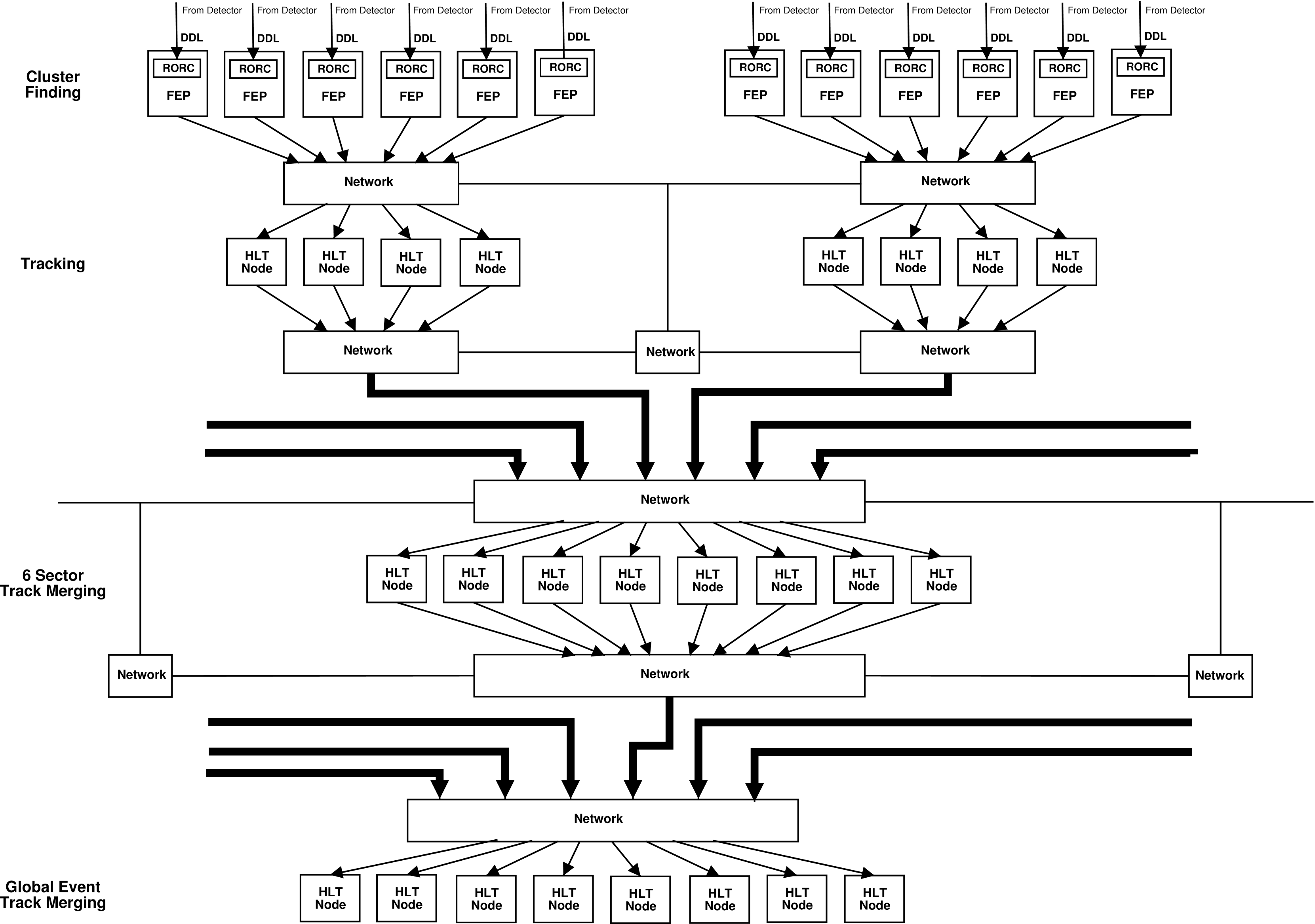
A sample architecture based on the assumption that all the analysis will be executed in software is shown in Fig. 2.2 for data from the TPC alone. The assumptions made for the amount of CPUs required for each step of processing are based on one hand on interpolations [93] from data of the Level 3 trigger at the Solenoidal Tracker at RHIC (STAR) [94] detector at the Relativistic Heavy-Ion Collider (RHIC) [95] accelerator at Brookhaven National Lab (BNL) [96]. On the other hand they are based on detailed simulations of the expected detector response in ALICE [97]. As can be seen in the figure, the cluster’s topology is built in a tree-like structure where successively larger parts of an event are processed and merged as one approaches the tree’s root. At the root of the tree the trigger decision is made based on the derived physics quantities of the given event. This tree structure is a natural choice given the segmentation of the TPC and the hierarchical nature of the analysis, which can easily be divided in multiple separate steps.
At the top one can see the FEPs for two slices with the DDLs and RORCs for the 12 patches needed. Two processing steps are performed on the FEPs. The run length encoded raw data is unpacked and then cluster-finding is done on the unpacked data to determine space-points of charge cluster depositions along particle tracks. This spacepoint data is then transported over a network to the next processing stage. On these next nodes an analysis is made to find track segments in each patch’s spacepoints that describe the particle tracks going through the TPC. For fault tolerance reasons with regard to the failure of nodes the spacepoints from one patch are distributed among the four nodes in the tracking group. Segments of tracks produced by six neighbouring tracking groups are then distributed to the next group of eight nodes. In this group the track segments from the six groups are merged to longer track segments over the respective six slices in the TPC. The data produced from the six groups of track merging nodes is sent to one last group of eight nodes where the data from all track merger groups is again merged to form the data of the complete event in the TPC. Based on this data these global mergers can make the HLT trigger decision. In this setup 216 FEPs would be present with an additional 144 nodes for tracking. Six additional groups of eight nodes are needed for track merging of a slice sextett and a final group of eight nodes for global event merging. In total this setup would thus require 416 nodes for the HLT.
All data from ALICE sub-detectors is read out upon an L2 trigger accept decision and is subsequently present in both the DAQ and the HLT. There is thus no need for a fixed latency or an upper bound on it for the HLT decision. The main memory of the FEPs will be used as derandomizing buffers for the events and event fragments. With memory sizes of several gigabytes expected for PCs when ALICE and the HLT will be activated, one PC will be able to store several thousands of event fragments read out from a TCP patch via one RORC/DDL. Nonetheless an average latency over all events will be enforced, determined by the event buffers, the average processing time, and the input data rates.
The HLT will consist of a farm with a large number of commodity PCs. Each of these individual PCs must be regarded as a relatively unreliable component and can fail at any moment. Experience with a small cluster in Heidelberg and elsewhere [98] [99] suggests a failure of one node at least once a week in a system of that size. Therefore the HLT needs a fault tolerant architecture that can cope with the loss of any node and still continue working. For the processing nodes a good approach is to distribute each task among a group of several nodes. An example for this are the track finding nodes in the sample setup in Fig. 2.2. Each FEP distributes its data among multiple nodes in the track finding group by sending incoming events on a round-robin basis to them. If one of the nodes fails this is noticed by a supervising instance informing the FEPs, which then can distribute data sent to that node among the remaining target nodes. Any new incoming data would also be distributed among the remaining nodes only, until the FEPs are notified that the failed node is available again. This node failure would thus cause no total system failure of the system but just a higher load on the remaining tracker nodes and maybe a slightly reduced event rate corresponding to the loss in processing power of the failed node. The capabilities of the HLT system as a whole would not be significantly influenced.
For the FEPs a different approach is necessary as each DDL ends in exactly one FEP. One simple solution to this problem is a kind of standby node equipped with RORCs, into which DDLs from failing nodes can be plugged. This of course would have to be done by manual intervention by a technician. But this approach would not prevent the loss of the raw data on the FEP at the time of the failure. An extension of the previous approach is to copy the raw data from an FEP immediately after it has been received to one of the other nodes in its patch group. In principle it would even be possible to use a device-to-device copy in which the RORC directly communicates with the networking adapter connected to the second node. The viability of this and other approaches will have to be analysed before a decision is made regarding this. But one major feature of any architecture chosen for the HLT must be the tolerance with respect to the failure of single nodes in the system and the lack of single points of failure in it.
The transport of the data through the HLT will be orchestrated by the software framework presented in this thesis. Due to the flexibility necessary with regard to different setups and changing analysis requirements, the framework must be very flexible and should allow easy changes in its configuration of the data flow. Similarly it should take into account the unreliable nature of the single nodes and be prepared to recover from the loss of any of them as detailed above. Furthermore, as the task of the system is the analysis of large amounts of data that will require large amounts of CPU power, the framework should be as efficient as possible and not use up too much CPU time for just the transport of data through the system.
2.2.3 CBM Project
The Compressed-Baryonic-Matter experiment [100] is a detector intended for the future High-Energy-Storage-Ring [101] (HESR) accelerator at the Gesellschaft für Schwerionenforschung (GSI) in Darmstadt [102]. Its primary research goal is the investigation of highly compressed nuclear matter, that can be found for example in neutron stars and supernova explosion cores. The HESR is designed to provide a dedicated heavy-ion accelerator with a number of parameters exceeding those of existing dedicated HI accelerators, like beam intensity, quality, and energy. The aim is to investigate new regions in the baryon-phase-diagram such as the quark-gluon-plasma and the areas of higher baryon densities. For this purpose the energy range between to per nucleon is investigated for a number of criteria, like exotic states of matter or the critical point indicating a phase transition from the quark-gluon-plasma to higher densities.
For the CBM detector the general HESR research goals are addressed by the simultaneous measurement of several observables sensitive to high baryon density effects and phase transitions. Amongst others particular attention is given to the following areas:
-
•
The parameters of penetrating probes, like light, short lived vector mesons decaying into electron-positron pairs, able to carry undistorted information from the dense hadronic fireball
-
•
Strange particles
-
•
The collective flow of all event observables
-
•
Event-by-event fluctuations of particle multiplicities, particle phase-space distributions, the collision centrality, and the reaction plane
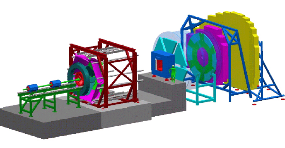
The CBM detector will basically consist of a magnet, silicon pixel and strip detectors, a RICH detector, TRD detectors, and an RPC Time-Of-Flight (TOF) wall detector, placed in line behind a fixed target in the beam as shown in Fig. 2.3. Unlike ALICE CBM is a fixed target experiment and thus does not need to provide a coverage around the collision point. The setup is designed to measure hadrons as well as electrons for beam energies up to per nucleon with a large acceptance. Particle tracking and momentum determination will be performed by the seven layers of silicon strip and pixel detectors inside the magnetic field located close to the target. In the remaining three detectors (RICH, TRD, RPC TOF) located downstream of the magnet, particle identification will take place, with the RICH and the TRD being used for general electron and high-energy electron identification respectively.
For the CBM readout a high level trigger or event filter farm using similar principles as for ALICE (PCI readout, a large Linux PC-cluster) may be used. In such a setup the use of the framework presented in this thesis is a possibility due to the framework’s generic design and the flexibility of its “pluggable” component approach.
2.2.4 PANDA Project
The Proton-ANtiproton-at-DArmstadt (PANDA) experiment [103] at GSI is designed to study collisions of protons () and anti-protons () with three primary physics goals:
-
1.
To study the behaviour of the strong force binding gluons and quarks together in hadrons, the collisions will be monitored for charmonium and other short-lived particles. A detailed spectroscopic analysis will then be performed on these particles with the aim of obtaining new results for the characteristics of the strong force at medium and longer distances as well as the origin of the quark and gluon confinement in hadrons.
-
2.
By studying high-energetic collisions it is expected to generate new data to determine the origin of the hadron masses, of which only a small part, e.g. 2 % in the nucleon, can be attributed to the valence quarks in each hadron.
-
3.
The third main goal is the search for exotic new forms of matter predicted by strong force theories, such as glueballs that consist only of gluons or hybrids that contain two valence quarks and one gluon.
For the PANDA readout the same statement for a potential high level trigger or event filter use and architecture applies as for CBM. This includes a corresponding use of the presented framework in such a system. One specific application could be searching for and selecting events in an online analysis that contain a charmonium particle.
2.2.5 Relation To Other Experiments
Other high-energy and heavy-ion experiments also use a system providing high level trigger functionality. The ones most related to ALICE are the ATLAS [104], [105], [106], CMS [107], [108], [109], and LHCb [110], [111], [112] detectors, currently also being built for operation at the LHC [55], and the STAR [94] heavy-ion detector at RHIC [95].
STAR is in operation at RHIC since 2000 and therefore belongs to a different generation of detectors compared to ALICE. It is, however, the newest heavy-ion detector currently in operation. The architecture of its Level 3 Trigger [113] [114] is characterized by a separation into Intel i960 processors on receiver boards and a PC farm with Alpha CPUs, all connected by Myrinet. Cluster finding is performed already on the i960 processors, and tracking is performed on Alpha PCs using the clusters received from the i960s. The L3 trigger’s task is to reduce the raw events of approximately 15 MB occuring with a rate of about 100 Hz to a rate of roughly 1 Hz.
ATLAS and CMS are two general purpose detectors whose main task is the search for the Higgs particle and signatures of physics beyond the Standard Model of particle physics. The ATLAS High Level Trigger [115] is separated into a Level 2 trigger and an Event Filter farm, both consisting of standard PCs. Together these two systems have to reduce the HLT input rate of 100 kHz events to the order of 100 Hz. A full event is between 1 MB and 5 MB in size, resulting in an output data stream of a few hundred MB/s. Data rate into the Event Filter is between about 600 Hz and 3.3 kHz, depending on the details of operation. An event switching network is located between the Level 2 trigger and the detector’s front end electronics so that a Level 2 node can request any fragment of an event needed. Between the front end electronics and the Event Filter farm an event building network is present so that the Event Filter farm operates on completely assembled events and does not have to perform any event merging itself. The disadvantage of this approach is the requirement of a high bisection bandwidth between the front end electronics and the Level 2 and Event Filter farms. As the network technology Ethernet has already been chosen for most parts of the system.
Expected event sizes for CMS are also about 1 MB. Input and output event rates for its HLT [116] are 100 kHz and 100 Hz, similar to ATLAS. An event builder network is used here as well to connect approximately 700 modules attached to the detector’s front end electronics with the HLT nodes. The HLT therefore will operate also on completely assembled events and will not perform any event merging or building itself. For the network technology the focus at the moment lies on Ethernet or Myrinet, both of which are investigated more closely.
The last of the three other LHC experiments, LHCb, operates with very small event sizes of around 100 kB. Its High Level Trigger [117] has to reduce the event rate from 40 kHz to 200 Hz. Since the output of the HLT are raw event data as well as event summary data the resulting output data rate is 40 MB/s, relatively low compared to the other three LHC experiments.
As can be seen from the above descriptions, these four experiments’ HLTs differ in at least one crucial parameter (required input or output data rates, event rate, or architecture) from what is required for the ALICE HLT.
2.2.6 Online Video Processing & Image Generation
Next to the use in high-energy and nuclear physics trigger systems other applications for the presented framework are also possible. Tasks that can be split up into sequences of parts which can be processed in parallel and/or in a pipelined manner are areas where the software is well suited to be used. Examples of such applications are online video processing and image generation, with four major uses:
-
1.
Decompression of a received, highly compressed video stream for display
-
2.
Compression of a video stream before transmission or storage
-
3.
Application of one or more filters to a video data stream before it is displayed
-
4.
On-the-fly rendering of 3D graphics into video streams for display or transmission
The general principle for the use of the framework follows a similar pattern for all of these four applications. A node receives data from an external origin and acts as a data source for the required number of processing units by distributing the data among them. Each of these processing units sends the output data resulting from its operation to one data destination. This destination node collects the data, assembles it into the correct order, and performs the desired action with it. It would even be a possibility to use two processing nodes for each sub-task, one of which performs a lower quality form of the operation that can be completed in a significantly shorter time. If the normal, higher quality data is not received on time at the destination the low-quality backup version can be used instead.
Video Decompression
In the first of these applications, online video decompression, the data input is the compressed video stream, received in the data source either by a specialized or commodity network or a specific readout device. The produced output data takes the form of a sequence of images, to be displayed on an output media.
Video Compression
For video compression the input is a raw video stream received most likely by a special purpose video readout device or receiver adapter. Output is a compressed video stream that can be written to disc, broadcast, or sent over a network to a number of receivers.
Video Filter Application
In the application of filters to a video stream input and output can both be a stream of either compressed or uncompressed video data. This stream is received and (re-)transmitted in the corresponding form as described for the previous two entries.
3D Image Generation
For image generation the source data are 3D scene descriptions either stored and read from a file or received from a generator system, either based upon a preset programm or following an operator’s input. The output is a video stream for storage or immediate display.
Chapter 3 Overview of the Framework
3.1 Introduction to the Framework
This thesis describes a framework that has been written for distributed online data processing in clusters as described in the previous chapter. One of its main characteristics is the focus on data driven architectures and applications in which elements can receive input data from other preceeding elements and produce output data for consumption by succeeding ones, as depicted in Fig. 3.1. Further emphasis during the framework’s development has been placed on efficiency, flexibility, and fault tolerance. For efficiency in this context the focus is primarily set on the reduction of CPU cycles used in the framework for the transport of data, to keep as much CPU power available for processing of data according to an application’s requirements. The requirement for flexibility is implemented such that the framework consists of a number of independent software components that can be connected together, without recompilation and even during runtime of the system, supporting a high adaptability in its configurations. Finally, fault tolerance of the software means that the framework has to be able to handle and recover from errors as autonomously as possible and that it should not contain any single points of failure. Instead the framework should be able to reconfigure itself during runtime to work around the faulty spot, aided by the dynamic connection ability described previously. In the following three sections of this chapter the most central design decisions and emphasises of the framework are detailed, followed by overviews of the components making up the framework and its software architecture.

3.2 Framework Design Considerations
A major point of attention and optimization during the design and implementation of the framework has been to avoid unnecessary overhead, mainly usage of too much CPU time and memory bandwidth. The suppression of these effects as far as possible is important since the framework is basically a means of getting data to the right place at the right time for its first intended use in the ALICE High Level Trigger. Considering the HLT’s purpose, i.e. the analysis of that data, and the size of the data involved, any amount of processing saved can substantially reduce the size of the whole system needed to process the required quantity of data, and a reduction of a system’s size also implies a reduction of its cost.
Furthermore the software has been optimized for a high throughput rate of events in a system. It has not been optimized for latency, i.e. the time elapsed between the event’s entering of the system and the HLT’s trigger decision for that event. The reason for this decision is that the HLT will be operated in a stream mode where new events will come in continuously. In such a system latency can be balanced by sufficiently large buffers to hold events that have been processed by one stage while the next stage processes preceeding events. This argument is made with the background that the recent and projected future development of memory size shows a steady increase following Moore’s Law. The increase in size is accompanied by a development of memory cost so that the price of the doubled amount of memory is at most only slightly more than the price for the original amount. Memory bandwidth in contrast can be scaled by the same amount, but this comes at a much increased cost and is not easily available for COTS PCs.
Another important point that has to be considered for such a system is the available memory bandwidth. As described in section 2.1, the available bandwidth of memory in PCs has not increased by the same factor as the CPU power. In theory CPUs are able to operate much faster than in reality where they are slowed down waiting for memory accesses. Caches have helped to resolve the situation partially and, depending on a program’s memory access pattern, effects may be more or less pronounced. In order to partially compensate for and work around the problem, trade-offs have been made in the framework that sacrifice amount of memory used over memory bandwidth. The motivation for this is the same as in the previous paragraph, memory size is cheap while memory bandwidth is not.
To allow a flexible and easy operation and configuration of a system using the framework as well as an easy customization, the framework should be composed of relatively small components, that can be connected together using a defined common communication interface between components. As such a system has to run distributed over the nodes in a cluster, a mechanism to allow components to communicate across nodes is needed as well. For efficiency reasons the communication between components has not been generalized to use a communication mechanism that would also work between nodes. Instead an efficient communication mechanism has been chosen that works only locally and special bridging components have been developed to connect components across nodes.
For the interface between the components a number of requirements have been specified:
-
•
A data producer should be able to feed multiple consumers to allow easy monitoring of both the framework’s and the analysis code’s correct functionality.
-
•
For efficiency reasons, only data descriptors should be exchanged between local processes, with the data itself kept in shared memory. As the data is potentially very large, especially in the case of the ALICE HLT, this requirement serves the purpose of preventing copy steps of the data between components.
-
•
Two kinds of data consumers should be supported:
-
–
Blocking consumers, called persistent subscribers, which need to access the input data until they have finished processing it. These are the actual analysis components that need to work on event data until the analysis is finished.
-
–
Monitoring consumers, called transient subscribers, that do not need to process every event and have to tolerate overriding event releases by the producer. These components can be attached as taps at any point in the data stream, statically as well as dynamically. An example of this is shown in Fig. 3.2.
-
–
-
•
Where possible producers and consumers should be identifiable by name rather than by numbers to ease setting up and debugging.
-
•
The design should be object-oriented to make use of the advantages of object-oriented software development like reuse and encapsulation.
-
•
Actual communication between processes should be hidden behind an abstract interface to allow an easy exchange of the underlying communication mechanism without having to change the upper layers.
-
•
It should run at least on the Linux operating system on Intel compatible CPUs as a baseline.
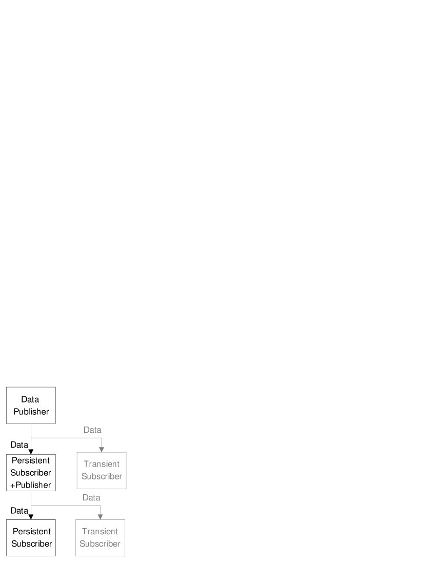
Since there is currently much development in the area of cluster interconnect and networking technology suitable for a system using the developed framework, such as the ALICE HLT, no decision has been made yet for a specific networking technology to be supported. Instead it has been decided that any inter-node communication is to be hidden behind an abstract communication interface that supports communication implementations using different networking technologies and protocols. This approach is also desirable with respect to flexibility, as it allows to setup a cluster for the framework with any supported network technology. It also allows easily to write implementations for new additional network interfaces that can be used by any system using this framework without changing the framework components.
Concerning the usage of network communication in the framework, two separate types can be distinguished. The first of these two types, the transport of the actual data to be processed, in general produces the bigger data volume. For ALICE this is the event data and the minimum block size for TPC raw data would be of the order of several hundred kilobytes. The second type of communication consists of small messages being exchanged for control, setup, and handshaking purposes, with a typical size from several tens of bytes up to a few hundreds of bytes. Taking this distinction between the two communication types into account, the abstract communication interface has been designed to provide optimized functions for the transfer of small data, like messages, as well as large blocks of data.
3.3 Components Overview
The framework consists of a number of separate components, that can be combined into a running system to allow maximum flexibility in its configuration. This flexibility necessitates that the components communicate via a defined interface that supports connection during runtime. To allow a maximum communication efficiency and usability, this interface is based on shared memory for the data exchange, as described above, and named pipes for control messages, like the exchange of descriptors. Named pipes make it possible to address each process by a unique name without the need to construct and manage a separate namespace. Instead the operating system file namespace is used. At the same time pipes provide an efficient operating system mechanism for a process to wait for incoming data without polling and thus without consuming CPU cycles while waiting. Two major kinds of components currently exist in the framework, generic components, not specific for a particular task, and components developed for use in the ALICE High Level Trigger.
With the generic components one can again distinguish four types: data flow components, worker component templates, worker, and fault tolerance components. Data flow components do not modify the data passing through a system but are responsible for routing the flow of data in it. These include components to merge parts of events into one part, to scatter and gather data among multiple nodes, e.g. for load-balancing purposes, and to transport data between nodes over a connecting network. Worker component templates are provided in the form of three sample programs that can easily be extended for components which respectively produce data (data sources), receive data (data sinks), and receive, process, and produce new data (data processing or analysis components). The generic worker components are a number of components, partly based on the template components, that act as data source, sink, or processing components. Finally, the set of fault tolerance components is responsible for making a framework system tolerant against faults of framework components, hardware parts, or even complete nodes. Some overlap exists between the fault tolerance and data flow components as a number of the fault tolerance components are extended versions of data flow components, performing the same tasks with added functionality.
ALICE specific components are analysis components that execute the different stages of the detector data processing. Starting at the raw data read out from the detector, each component represents one step in the analysis process and accepts a specific type of input data. This input data is processed and another type of output data is produced. The new ouput data is in turn made available to the next step in the chain for further processing. After the last step has been executed, a fully reconstructed event is available as the base for the trigger decision.
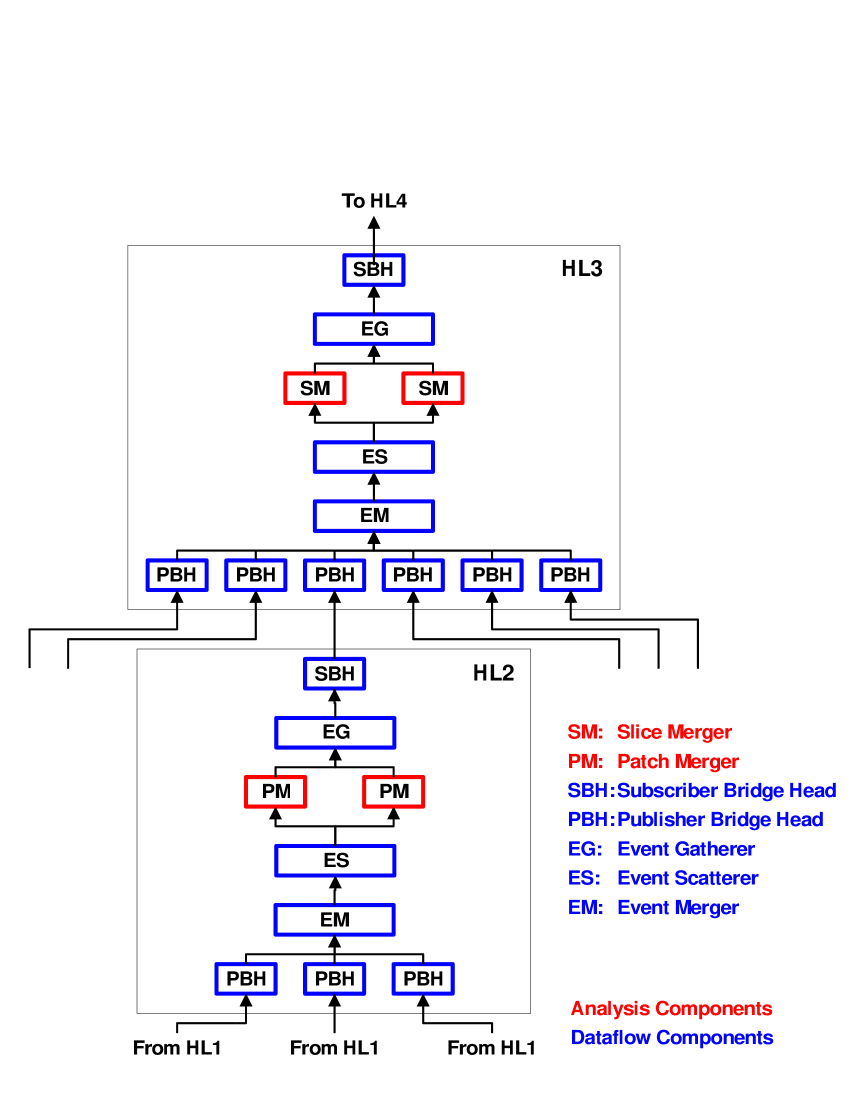
Fig. 3.3 shows a number of the framework’s components in a possible setup as it might be used in the ALICE High Level Trigger for the processing of TPC data. The figure shows two nodes in the central two hierarchy levels (HL) of an HLT configuration with several components running on each of them. A detailed description of the components is provided later in chapter 7. Components shown in blue are generic data flow components, while red ones are ALICE HLT processing components. One can see the data flow components that connect multiple nodes (SBH and PBH), merge parts of the same event (EM), and that scatter and regather event streams for load balancing (ES, EG). The two types of processing components in the figure perform different levels of merging, the first (PM) on the level of the subsector patches and the second (SM) merges a number of the sector slices. On the following hierarchy levels more merging components are present to reach a fully merged event at the end of the processing chain. As can be seen, the configuration makes use of the inherent structure and hierarchy in the TPC and its data analysis to arrive at a natural decomposition and distribution of the different processing tasks.
3.4 Software Architecture
From the software architectural side, the framework is divided into a number of distinct packages or modules, some of which are dependent on others. The relationship between the modules is shown in UML notation in Fig. 3.4.
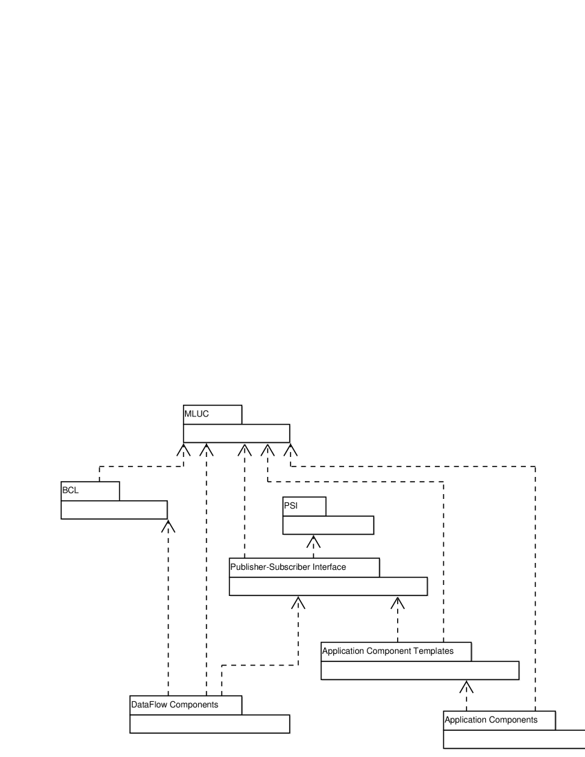
At the top of the figure are two basic modules, MLUC and PSI, that provide basic functionality and do not rely on any other module. The More or Less Useful Class library (MLUC) package is a C++ class library providing generic classes used in the other packages. One of the classes provided by MLUC is a thread class to encapsulate operating system functionality for creating multi-threaded programs. Also included is a string class, that actually provides less functionality compared to the string class present in the standard C++ library available with the GNU C++ (g++) compiler. The GNU class however is not thread safe and as all but the most trivial programs in the framework are multi-threaded it could not be used. Another major class in the package to be included here is a new vector class for handling of dynamic arrays. In most cases where the vector class is used, it is used in an almost queue like functionality, with items being added at the end and removed from near the beginning. With the Standard Template Library (STL) vector class, also distributed with the g++ compiler, this access pattern causes all elements after the one removed to be copied one element forward. Already for moderately large arrays this copying process takes up a lot of CPU time and obviously also uses up a lot of memory bandwidth. To change that situation the new dynamic array class was written, that trades off memory size used for the array for a reduction in used memory bandwidth, as outlined in the previous design section 3.2. The last major functionality contained in the MLUC library is a logging facility for programs. This logging facility is designed to have multiple severity levels of log messages and to have a negligible overhead when a severity level is turned off. Furthermore it features a modular system of logging targets to which messages are dispatched, that can be configured completely at runtime.
The second basic module, the PCI and Shared memory Interface (PSI), provides user level access to PCI bus devices as well as a shared memory interface. PCI devices that need to be accessed can be special readout hardware while shared memory is used to exchange data between framework components. The module consists of a library providing an Application Programmer’s Interface (API) together with a driver that performs the actual hardware accesses and operating system interactions. As the name suggests PSI’s primary purpose is to provide access to PCI adapter cards and other devices from normal user space programs. More specifically it allows to access the Configuration Space Registers (CSRs) of any PCI device, including bridges, as well as access to the memory and I/O regions described by the Base Address Registers (BARs) of PCI devices. Memory BARs as well as arbitrary physical memory addresses can be mapped into the address space of user space programs and can then be used like any normal program memory. Shared memory access is possible to two kinds of shared memory, the first of which is ordinary shared memory that can be located anywhere in the physical memory of the computer and does not need to be physically contiguous. The second type of shared memory is located in a memory area obtained by using the big physical area memory patch [118]. This patch reserves a single large physical memory region on system start and can allocate chunks of this memory to programs and drivers. The special characteristic provided by this patch is that any memory allocated from it is actually contiguous in the physical memory, making it ideally suited for streaming access and for access by Direct-Memory-Access (DMA) capable PCI devices. This last point is especially important, as many SAN adapters are actually DMA capable and could transfer data from and to this memory without using the CPU. A tool library also contained in the package makes use of the basic functions in the driver to provide more complex higher level functionality together with a number of utility programs.
At the left side of the figure is the Basic Communication Library (BCL) module providing the abstract interface for communication outlined in the preceding section. This module is also a C++ class library, which contains an abstract base class defining general communication functionality. Function names in the library have been chosen to follow the widely known and used socket API of the POSIX [119] or Single Unix specification [120], [121], [122] where appropriate. The base class provides functions for performing a bind to an address that remote programs can connect to as well as functions for connecting to remote program’s addresses. Two further abstract classes are derived from this class, one for each of the two communication patterns from section 3.2, transfers of small message-like data or large blocks of data. Each of the two classes provides its own API adapted to its specific task. The message like API has functions for directly sending and receiving small structures to any address. With the block API a user first has to request memory in the remote buffer to store the data before it can actually be sent. From these two base classes in turn the classes are derived that contain the implementations of the APIs for actual network protocols. Currently both communication types are supported for the TCP protocol [22] as the most widely available baseline and for the shared memory SCI interface [13] as an example of a low latency and low overhead SAN technology. More details about this module can be found in chapter 5.
While the previous three packages provide functionality that can be used in many projects, the remaining four packages, covered in chapters 6 and 7, contain the code of the actual data flow framework itself. Utilized by the other three modules, the Publisher-Subscriber-Interface module contains the implementation of the interface used by the framework components for communicating locally on one node. The interface is based on shared memory to hold the data to be transported between components and named pipes to send descriptors holding the location of the data to be exchanged as well as its size and type. It makes use of the publisher-subscriber pattern [123], also known as producer-consumer principle. The Publisher-Subscriber-Interface package provides a set of classes that encapsulate the interface and that can be easily used in programs that want to communicate with components in the framework or in components themselves. Components using this interface are supplied by the remaining three modules. Of these modules the Data Flow Components module also relies upon the BCL module. Components in this module are used to shape the flow of data through a system built with the framework. One component merges data streams containing different fragments of the same event so that one event stream with larger fragments or complete events is produced. Two other components can be used to split up a stream of events evenly into a number of streams of lower rates and to later reunite them into one large stream. This can be used for load balancing purposes with each of the smaller streams being handled by a separate node or CPU. The final pair of components is used to form a bridge between two nodes to transparently connect components on the nodes using the publisher-subscriber interface. For this purpose the first of these components uses the common interface for component communication to obtain the data to be sent. This received data is then transmitted to its counterpart component on the peer node, using communication classes from the BCL library. Data received by the component running on this node is again made available to other components, also by way of the component interface.
The second module using the Publisher-Subscriber-Interface module is the Application Components Template module that provides templates for application specific or user components. These components are needed so that a user building a system with the framework can incorporate components with functionality specific to the setup and tasks of that system. Three basic types of these user components can be distinguished: data sources, data sinks, and analysis or processing components. Data sources are components that accept or read out data from a source external to the framework. Sources can be simple files, network daemons, or special hardware such as the ALICE RORCs. This data is made available to further framework components, these data source components thus feed a system with data to be processed. Data sinks in analogy are components that only accept data from the framework to perform a specific task with it. Possible tasks are writing data to files on disk or a database or sending it via a network to another system. Sinks and sources are in principle the opposite endpoints for data in the framework. Analysis components in contrast are located in the middle of the framework. They receive data from other components and process it, either producing and outputting new data or just outputting the same data again. Its output data can again be used as the input for other components. In the Application Components Template module templates for all of these three types of application components are contained, providing most of the functionality needed to include specific components in a system. A user only has to add custom code to provide the data for sources, handle the received data for sinks, and produce new output data from received one for analysis components.
The Application Components package is making use of the Template module and supplies a number of working user components based on the templates. Some of these components can be used directly in production systems while others are intended for development and testing. An example of the second category is a data source file publisher component that uses a set of files specified on the command line and publishes them round-robin into a system’s data flow chain. A contained component that can be used in a production system is a data sink that accepts events and, after a configurable number of events have been received, calculates the average rate of received events and reports that rate using the logging facility of the MLUC package.
Chapter 4 Utility Software
4.1 PCI and Shared Memory Software
There are two types of applications requiring a special device driver in the context of a data flow framework: Access to specific readout hardware, including prototype and development boards, and use of large shared memory areas for interprocess exchange of data. For the last usage the operating system supplied shared memory, such as System V Shared Memory [120], [121], [122], [124], could in principle also be used. However, under Linux at least there seems to be a restriction to a maximum segment size of about 32 MB. This restriction makes the approach unfeasible for the use in the desired application, where buffer sizes of several hundreds of megabytes are needed to store a sufficiently large number of data blocks. As far as the first application is concerned, programming a separate device driver for every piece of hardware is the more elegant approach, but is the most undesired too, due to the complexities and overhead involved in the programming of device drivers compared to ordinary user space programs.
The PCI and Shared memory Interface (PSI) software described in this section is used to provide the handling of shared memory for the publisher-subscriber interface and the framework components described in chapters 6 and 7 respectively. For the ALICE HLT the module will additionally be used for the development of programs accessing the RORC readout cards. An item that at the moment is not supported by the software is interrupt handling.
To provide a background for the explanations of PSI software functions, parts of this section contain a brief overview of some characteristics of the PCI bus. For more in-depth explanations or specifications please refer to e.g. [21] or [125].
One consequence associated with the interface are the security risks it presents, since it allows any user of a system who has privileges to access the driver unrestricted access to any memory area of the system, even operating system memory. This memory access could be used to gain full access privileges to the system and access any desired data. One way to prevent or restrict this, is to make the device node used to access the driver available only to a trusted group of users and regulate access in this way. At a later stage, the driver might be modified in such a way, that it allows access only to a certain set of devices and shared memory segment areas. This set of PCI devices might be specified with the PCI vendor and device id, unique to each PCI device. Both restriction sets, memory and devices, could be either compiled into the driver itself or for somewhat greater flexibility could be specified as parameters when the driver is loaded.
The interface operates on the principle of regions and a virtual device tree. A region corresponds to each type of access one wants to perform and is analogous to a file handle. It is necessary to open a region before being able to access any device or memory area. Each region allows access to only one device or area of memory associated with it. Which device or memory area has to be opened is specified using a string that describes a node in the virtual device tree. A graphical sketch of the tree structure is shown in Fig. 4.1. Fig. 4.2 shows the strings used to specify the corresponding device regions.
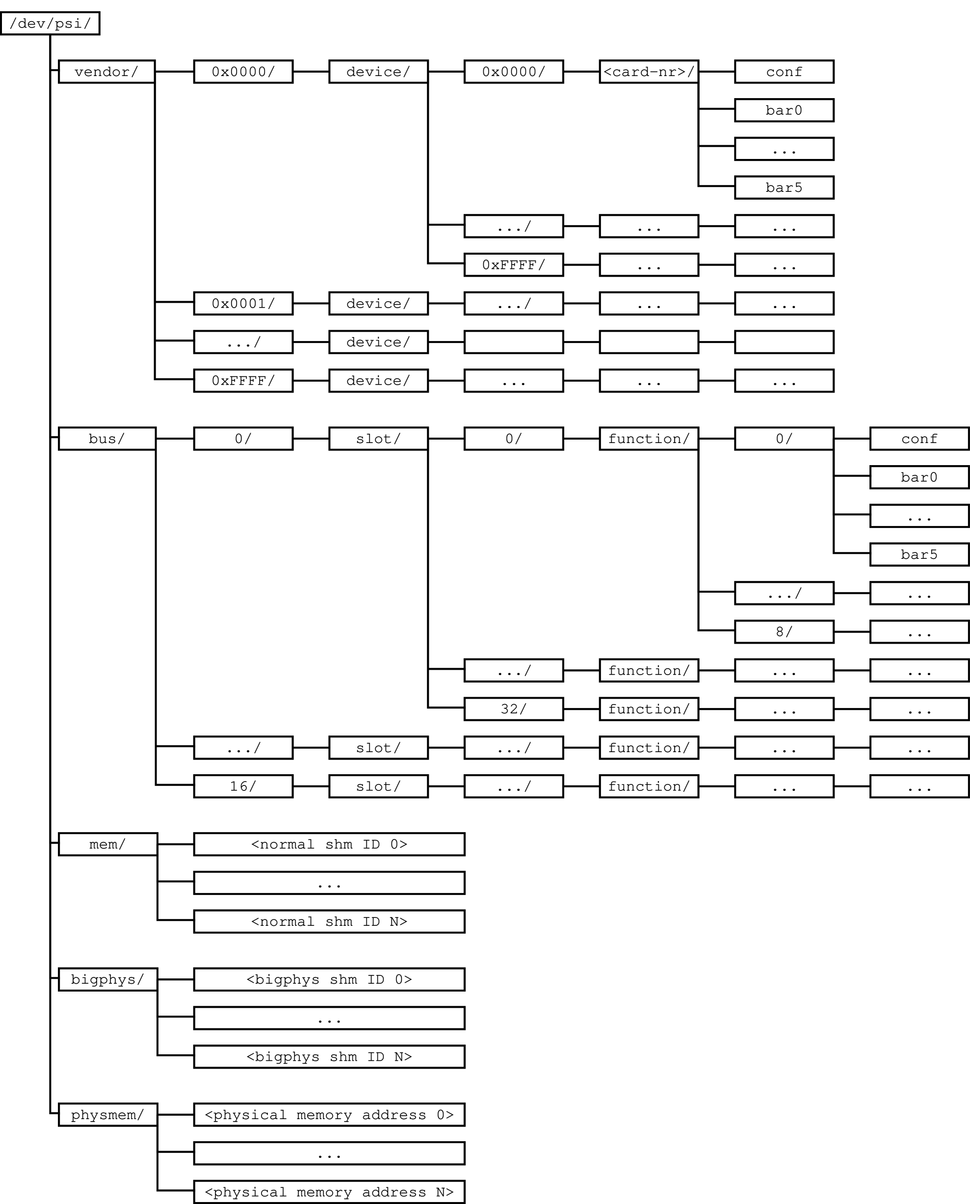
/dev/psi/vendor/<PCI vendor id>/device/<PCI device id>/<card nr>/conf /dev/psi/vendor/<PCI vendor id>/device/<PCI device id>/<card nr>/bar<bar nr> /dev/psi/bus/<bus nr>/slot/<slot nr>/function/<function nr>/conf /dev/psi/bus/<bus nr>/slot/<slot nr>/function/<function nr>/bar<bar nr> /dev/psi/mem/<shared memory id> /dev/psi/bigphys/<bigphys shared memory id> /dev/psi/physmem/<physical memory address>
PCI devices that have to be addressed can be specified in two ways, logically and physically. Logical addressing is done using a device’s vendor and device ID, unique 16 bit numbers. The vendor ID is assigned by the PCI group and the device ID is assigned by a device’s vendor so that each manufacturer and each device have its unique ID. With the combination of vendor and device ID it is ensured that no two types of devices in a PCI bus can be mixed up. But it is of course still possible that multiple cards of the same type are inserted into a system. For such a case a card index is available to specify which of the present cards should be used. This is the format shown in the first two lines of Fig. 4.2.
Physical addressing, also called geographical addressing, of a card makes use of the architecture of the PCI bus. A system can actually contain multiple PCI busses, up to a maximum of 16, numbered starting at 0. Each bus in turn can have a number of slots for plug-in cards, also numbered from 0 up to a maximum of 32 slots. Fixed built-in devices are still assigned a number in the same range, called slot/device number. Finally, each device can contain multiple functions, it can basically be divided into multiple sub-devices up to a maximum of 8. Addressing a device with these three parameters is done using the syntax shown in the third and fourth lines in the figure.
Once a certain device or card is specified, the part of the device that has to be accessed must be specified. A PCI device’s configuration can be written or read through its configuration space, a 64 byte region present for each device’s separate function or sub-device. In addition to this configuration space, each device’s function can offer up to six address regions for accessing its specific functions. These address regions can be either memory mapped regions, addressed like computer’s RAM, or they can be I/O regions. As the I/O address range is very limited many devices use memory mapped address regions. The six accessible address ranges of each device are specified in registers in the device’s configuration space called Base Address Registers (BARs). Frequently the term BAR is also used to specify the actual address areas that a register points to. For both of the above methods of addressing a PCI device, it is possible to either specify the configuration space to be accessed, shown in the first of each pair of lines, or to access the area pointed to by one of the available BARs.
Next to PCI hardware, the interface allows also access to shared memory areas. Two different types of shared memories are supported: Ordinary shared memory and memory accessible using the big physical area patch [118]. Ordinary shared memory does not differ much from other interprocess memory, like e.g. System V ShM. It is located in normal RAM and is available on every system without modifications to the operating system kernel. A shared memory region of this type is opened by using the syntax of the /dev/psi/mem line in Fig. 4.2. The shared memory ID in this line can be any string, unique for each shared memory region to be opened. To share a memory range programs have to open a region using the same ID. One drawback of this shared memory type however is that it can be limited in the maximum size possible for a segment. System V shared memory for example has failed to be allocated beyond a size of around 32 MB in tests. Another potential disadvantage is the fact that although this type of shared memory appears contiguous in the virtual address space of a user program it may be scattered in the actual physical RAM.
Bigphys shared memory in contrast does not suffer from these two problems. It is in principle similar to the standard shared memory and its regions are also identified using a string ID. The major difference is that bigphys shared memory is allocated via a kernel patch, the big physical memory area patch. This patch allocates a specified number of memory pages at the start of the system, with the advantage that the allocated memory actually exists as one large block in physical memory. Other drivers, in this case the PSI driver, can request a certain amount from that allocated memory. If this request can be fulfilled the returned memory range will be contiguous as well and will neither be swapped out nor removed by the system from its physical address for any other reason. The continuity of that type of memory has the advantage of being well suited for data streaming purposes and for accesses from Direct-Memory-Access (DMA) capable hardware. DMA capable hardware typically receives a pointer to a memory area and then either reads data from or writes data into that location. One example of DMA capable hardware is the ALICE RORC, that receives a pointer to a large data buffer in the computers RAM and copies received event data into that buffer on its own without copying being done by the system’s CPU.
Immediate physical memory addresses that can be anywhere inside the system’s memory address space — 32 bit for typical PCs — are the last type of region that the PSI driver can access. The driver performs no check on the presence of actual hardware accessible at that address. Write accesses to unused addresses will succeed, without the data being written anywhere. Data read attempts will return invalid data, in most cases data with all bits set.
After a region has been opened, its size needs to be set for the region types where this cannot be determined automatically. This is the case for the three memory region types, normal shared, bigphys shared, and physical memory. PCI BAR regions and configuration space regions are sized automatically. The respective BAR size to be used is determined conforming to the PCI specification from the device’s configuration space. Configuration space regions are sized to the default value of 64 bytes. For a sized region it is possible to read data from and write data to it. These read and write accesses can be done in units of 1, 2, or 4 bytes and can be any arbitrary multiple of the unit size. For all memory types, including memory BAR regions, it is also possible to map them into the user program’s address space. The mapping returns a pointer to the program that can be used like a normal pointer variable in a C program. It provides a very direct and fast access to the memory region concerned, as there is no operating system call associated with each region access, making this the most effective and easiest way of hardware access.
Built on top of the basic functions provided by the PSI library is a further library, the PSI Tool Library, that makes some higher level functions available. Included functions address various tasks associated with PCI configuration spaces. The most basic ones of these are for reading out configuration spaces directly into data structures with variables corresponding to the decoded elements of the configuration space. These structures can be printed out in a human readable form using further available functions. Other functions in this higher level library deal with the sizes of regions pointed to by PCI devices’ BARs, which can be determined by specific read and write accesses to a device’s configuration space. These BAR region sizes, together with flags that can be set for a BAR, can be read out and printed by another set of functions. Defined flag values can specify whether two 32 bit BAR addresses have to be combined to a 64 bit address and whether a certain memory BAR is prefetchable (cacheable) or not.
In addition to determining the size of a region pointed to by a BAR it is also possible to configure a device’s BAR by assigning an address under which that region will be accessible. This assigned address has to point to a free memory region of a size large enough to accomodate the needed window in order to avoid conflicts. In order to ensure this the library function first determines the sizes of the memory regions needed and scans all devices on the system’s PCI bus(ses) to determine the address ranges already in use by other devices. If the device is located behind one or more PCI bridge devices, the library will take further steps to configure the region so that it will be inside the address window passed by the bridges to devices behind it. Once the used address ranges are determined, the remaining free ones will be scanned for the best fitting window, the smallest one still large enough to take up a region of the necessary size. During this process the necessary alignment of the address according to the PCI specification is also taken into account. Finally, when the device itself is properly configured, the function will again scan the bus for bridges in front of the device and configure their window sizes accordingly so that accesses to the device will pass through them.
Another function contained in this library can be used to test open regions by writing a number of patterns to it, reading back the data, and comparing it with the written data. If the data read back does not correspond to the data written, it is read a second time to get an indication of whether an error occured on reading or on writing. Four patterns can be written by this function:
-
•
Walking Ones, where one set bit is shifted once for each word written, e.g. 0x00000001, 0x00000002, …, 0x80000000, to each 32 bit memory location.
-
•
Walking Zeroes, where one unset bit is shifted once for each word written, e.g. 0xFFFFFFFE, 0xFFFFFFFD, …, 0x7FFFFFFF, to each 32 bit memory location.
-
•
Full Bits, where alternatingly data words with all bits set and all bits unset are written, e.g. 0x00000000 and 0xFFFFFFFF, to each 32 bit memory location.
-
•
Flipping Bits, where alternating data words with every odd or even bit set are written, e.g. 0xAAAAAAAA and 0x55555555, to each 32 bit memory location.
The final part of the PCI and Shared Memory software is a set of small user programs for access to most of the region types described above from a command line shell. This avoids the necessity of writing separate programs for small infrequent accesses, e.g. basic testing. The type of region to be accessed, the parameters required for that region type, and the data to be written are all specified via command line parameters. Data to be read is printed out normally. The first program in this set allows read and write accesses to a PCI device’s configuration space or its BARs as well as to physical memory addresses. Data read can be dumped in a format suitable for input as write data so that it can be written to a file and later to the same or another region. A second program can perform the test routine described in the previous paragraphs on the same region types as the read/write program. The final utility program reads an arbitrary data file and dumps it into a format that can be used as write data input for the read/write program. This allows any file, for example configuration data, to be written directly into a specified region.
4.2 The Utility Class Library
During the development of the framework the necessity arose for a number of utility classes with a sufficiently generic functionality to place them into a separate library, the More or Less Useful Class library (MLUC), so that they can be used in other projects as well. Some of these classes encapsulate existing system functionality with an object oriented (OO) interface while others encapsulate and supply new functionality. A third set of classes was written to replace or enhance classes from standard libraries either for performance reasons or because the standard library class did not work in a multi-threaded environment.
4.2.1 Function Encapsulation Classes
The Logging System
The first set of classes is designed to offer a fast logging system for programs to easily and flexibly dispatch informative messages to one or more destinations. Different levels of severity for messages are supported by the classes, ranging from fatal errors to debugging aids. Three main criteria have been set for the development of these classes: Normal operation of a system should be influenced by the logging system as little as possible, therefore the overhead of a message with a deactivated severity level has to be very low. Secondly, the system should support multiple message destinations in a manner transparent to the code performing the actual logging. Destinations should also be changeable at runtime, again transparently to the code using the logging system. The last requirement for the system was that the severity levels should be selectable independently of each other. In many systems of this kind deactivating a severity level causes all less severe levels to be deactivated as well.
LOG( MLUCLog::kDebug, "LogTest", "Msg 1" ) << "Log test message 1." << ENDLOG;
A code example of a logging message is shown in Fig. 4.3. The first parameter to the LOG call specifies the severity of the given message, in this case debugging severity, a list of the available levels follows below. Following the severity are two strings, the first specifying the origin of the message, the second holding keywords categorizing the message. After the LOG call the C++ stream operator << is used to pass the actual contents of the message to the system. To signal the end of the log message the ENDLOG constant is streamed into the system.
The requirement for individually selectable severity levels of the system has been implemented by using a single bit in a 32 bit number for each level, restricting the number of levels to 32. Currently six levels are used in the system. In order of decreasing severity these are fatal, error, warning, informational, debug, and benchmark. As these six levels should cover most of the occuring applications, the remaining 26 allow enough extension possibilities. Bits and thus levels can be set, unset, or queried using the standard bit operations in the C/C++ language. Most of these operations can be translated directly to one or two low-level machine instructions so that especially the frequently used query operation can be executed effectively.
As stated in the first paragraph, the first design criterion of the system was a very low overhead for logging calls with deactivated severity levels. The rationale for this requirement comes from the fact that the less severe messages, like debugging messages, are frequently used and as a result can occur very often during the runtime of the system. These message levels are typically activated only during the development and testing of a system or in case of errors, and not during normal production, as logging a message is generally very slow on the typical timescales of such systems. But to retain the ability to diagnose runtime problems it is not desirable to remove them from a production system completely, and so one takes the compromise of deactivating the severity levels concerned. In case of a problem they can be activated again during the running of the system. Although it will be impossible to completely eliminate any impact of messages with deactivated levels on system performance, it still should be kept as low as possible. This includes even the avoidance of a function call in such a situation if possible. The overheads resulting from various methods of calling a logging system are presented later in section 8.1.1. In a preceeding summary it can be stated that function calls have a much higher overhead than the method chosen here. However, despite all these efforts to make the system effective it should still be easy to use in programs.
#define LOG( lvl, origin, keyword ) if (gLogLevel & lvl) \
gLog.LogMsg( lvl, origin, keyword, \
__FILE__, __LINE__, __DATE__, __TIME__ )
To achieve the aims of low overhead for unused severity levels and ease of use, a combination of C preprocessor macros, C++ class methods, and overloaded operators has been chosen, partly hidden from users. The first important part is the macro definition for the LOG call, shown in Fig. 4.4, that hides an if-statement and a method call executed when the condition in the if-statement is true. This if-statement is mainly responsible for achieving the required effectiveness. In the if condition it is tested whether the bit corresponding to the message’s severity is set in the gLogLevel variable. gLogLevel is a global variable specifying the activated severity levels in a program. If the respective severity bit is not set, the rest of the logging statement will not be executed at all. For disabled severity levels the overhead of a logging call thus amounts to an if-statement with a test for a set bit. On Intel compatible processors the GNU C Compiler (gcc) (Version 2.95.3) translates this into the four processor instructions for an i686 (Pentium-Pro or later) processor shown in Fig. 4.5.
movl gLogLevel,%eax
addl $16,%esp
testb $2,(%eax)
je .L2612
The gLog object used in the LOG macro is not an object itself but a global reference. It points to an instance of the MLUCLog class, the actual interface to the logging system. This object also handles the dispatching of logged messages to the different message present destinations. By using a reference instead of the MLUCLog instance directly it is possible to transparently change the log message interface. For reasons of brevity the global MLUCLog instance will be referred to as the gLog object.
In the gLog object’s LogMsg method, called in the macro when a message is logged, the message is prepared. Four preprocessor macros are passed to the function in addition to the three parameters passed to the LOG macro: The name of the code’s originating file together with the line number in the file, and the time and date when it was compiled. Additionally the current date and time as well as the name of the host on which the program runs are stored. To ensure thread safety a mutual exclusion semaphore (mutex) is locked so that only one thread at a time can access the logging system. As the locking is only performed for messages actually logged, the impact on a running system should be minimal. The message content streamed into the logging system is stored in the gLog object until the ENDLOG identifier has been streamed. This causes the full message to be assembled and passed to the active logging destinations. After this has been done the logging mutex is unlocked again, releasing the logging system for access by other threads.
To achieve the final goal of multiple transparent logging destinations for the logging system, it has been divided into multiple classes: The MLUCLog class as the primary interface, the MLUCLogServer class as the abstract interface for message destinations, and classes derived from MLUCLogServer with the actual destination implementations. This division is shown in Fig. 4.6.
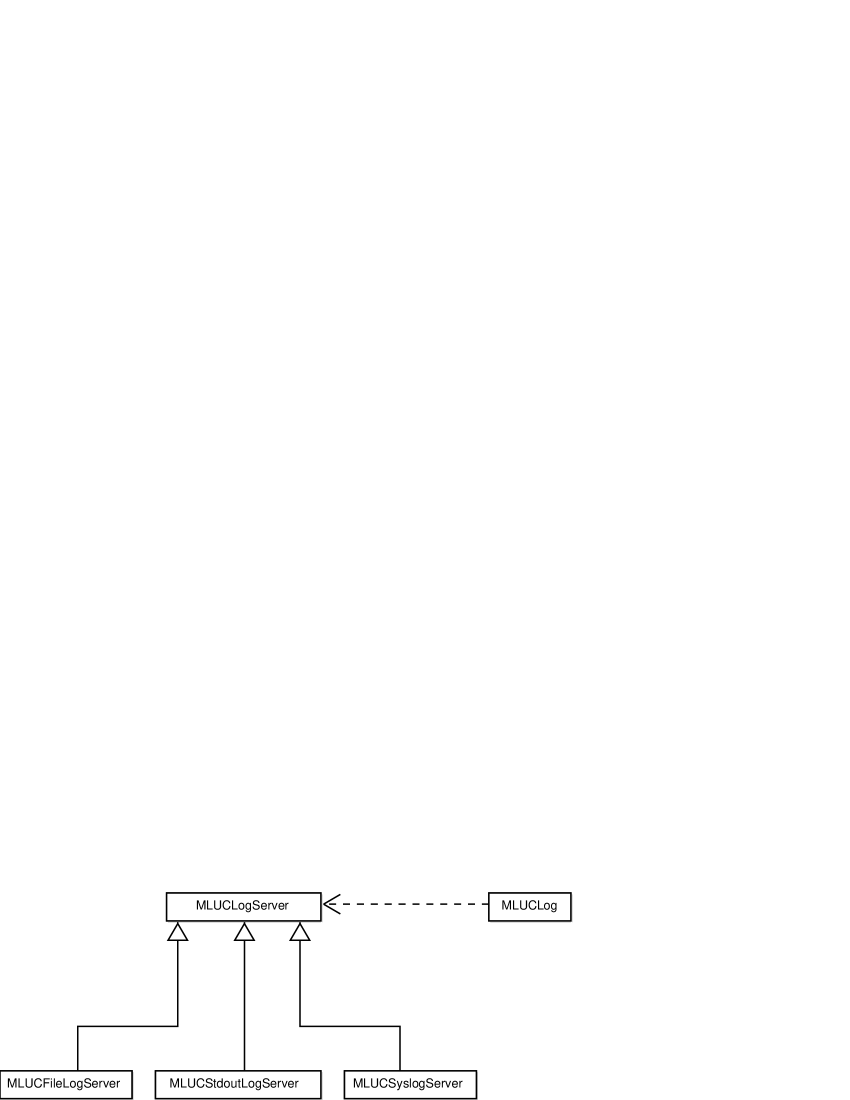
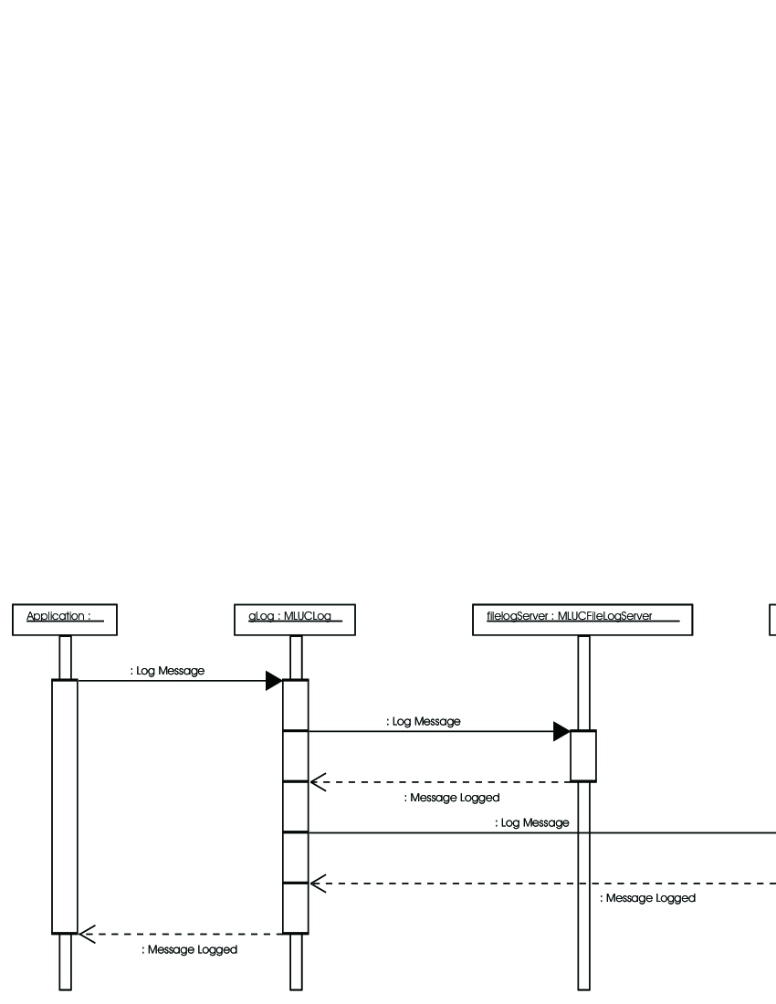
The global gLog object contains a list with pointers to instances of MLUCLogServer derived classes. Each of these derived classes is responsible for delivering log messages to a certain destination, examples of which are the standard output channel of programs, sets of files, or the syslog facility present on Unix computers. Instances of the classes corresponding to desired log destinations are registered with the gLog object, which enters them in its list of destinations. When the program makes a call to the logging system the complete message is assembled in the gLog object. Having received the message the object iterates over its list of registered MLUCLogServer destination classes, dispatching the message to each of them. After this the destination classes are responsible for delivering the message, e.g. by printing it to the standard output or writing it to a file. The interface to the destinations, the MLUCLogServer class, is hidden inside the logging system. Only when a class for a new destination has to be written has it to be used directly.
A sample sequence of a logging call is shown in Fig. 4.7. In this sequence an application makes a logging call for a message to the global gLog object. Two instances of MLUCLogServer derived classes are registered in the gLog object: an MLUCStdoutLogServer, printing messages to the program’s standard output, and an MLUCFileLogServer, writing the messages to a file. The gLog object sends the received message first to the MLUCFileLogServer object and then to the MLUCStdoutLogServer object. After the message has been dispatched to both registered MLUCLogServer objects the logging call returns control to the application’s code.
Depending on the implementation of the logging servers used logging a message might block a program, e.g. when a disk is full or when a network error for a log target node occurs. The currently provided servers will block in such situations, corresponding to their respective destination. To avoid blocking a log server implementation could make use of a background thread to for sending or writing of the data. Such a solution however could require the discarding of log messages when this background thread is blocked for too long.
Multi-Threading Classes
Most of the programs used in the framework consist of multiple threads for two reasons. Primarily, the motivation is to prevent programs from blocking completely when one part of a program blocks. This might occur when a system function used to communicate with another program blocks, for example because the communication partner has terminated. If on the other hand the program is multi-threaded, only the thread executing the communication can block. Care has to be taken of course that no other thread in the program will block because of waiting for a certain condition in the communication thread.
To facilitate multi-threaded programming and especially communication between threads in one program, several classes have been implemented in the MLUC library. MLUCThread, the first of these, has the purpose of handling of the threads themselves, e.g. starting and stopping. It uses the POSIX threads (pthreads) API [119], [120], [121], [122] and encapsulates it into a class providing methods for starting and aborting threads. An abstract (pure virtual) member function Run declared in the class is called when a thread is started, serving as the actual thread function, so that the thread is terminated when the Run function ends. Creating a new thread as a consequence involves deriving a class from MLUCThread and overwriting the Run method with the code to be executed by the thread. For integration with functionality in other classes, the template class MLUCObjectThread has been derived from MLUCThread. It uses another class type as its template parameter, accepting an object and a member function of that class in its constructor. In its Run method the specified member function of the given object is called, making that method the actual thread function.
For purposes of signalling between threads the MLUCConditionSem class implements a condition semaphore, also called a signal. Waiting for signals from other threads is supported by the class either with a specified timeout or without. When a timeout has been specified, the Wait function returns even when no signal has been received. Otherwise it will wait indefinitely for a signal to arrive before returning. To prevent race conditions between waiting for a signal and signalling, the MLUCConditionSem uses an internal mutual exclusion semaphore (mutex). It is acquired by default and is released atomically before a wait is entered. When an attempt is made to signal a thread waiting on this object, the mutex is tried to be locked as well. If no thread is waiting for a signal on the object, this will cause the signalling thread to block until another thread calls one of the object’s Wait functions. To support longer processing sections between waits, without blocking signalling threads, the class supplies two member functions for manual locking and unlocking of its internal lock.
In addition to these signalling features the MLUCConditionSem class also supports a notification data structure. This queue consists of a list of 64 bit data items. Items are added to the end of the list and queried or removed from its beginning. Using the queue makes it possible to provide a thread with a list of items to be processed by signalling it whenever a new item has been added to the list. To ensure thread safety while maintaining efficiency the notification data is protected by a separate lock, distinct from the internal lock associated with the signal/wait functionality. Internally the class uses the MLUCVector class covered later in this section, making use of the provided efficiency features of that class.
For inter-thread communication where exchanging single 64 bit values is not sufficient, a second First-In/First-Out (FIFO) communication class is available. The MLUCFifo class offers an interface for the exchange of data of any size between multiple threads. For efficiency reasons the interface is optimized so that it is not necessary to have the data available for a write call to be copied into the FIFO. Instead a location of a specified size is allocated in the FIFO and the pointer to that location is returned. The thread writing into the FIFO can then write its data directly without having to store it in a temporary location and copying it from there into the FIFO. After writing the thread calls a commit function that updates the FIFO’s internal tables, exposing the written data into the FIFO as available for reading. For thread safety the allocation and commit member functions of the class also perform locking/unlocking respectively so that only one thread at a time is able to write into it.
Reading works in a similar manner: When data is available for reading the responsible member function returns a pointer to the start of the available data. After the reading thread has finished processing the data it calls another function to free the accessed data. The free call also updates the object’s internal tables, marking the freed space as being available again for writing new data. Similar to writing, reading also involves a locking mechanism ensuring that no two threads can access the data simultaneously. To allow concurrent reading and writing separate read and write mutexes are used.
An MLUCFifo object contains two buffers for data, an ordinary and an emergency one, where the emergency buffer is typically rather small. On writing data it is possible to specify into which of the two buffers the data should be stored. On reading this is not possible, instead the emergency buffer is always checked first for the availability of data, and only if it is empty is the ordinary buffer checked. This mechanism ensures that it will always be possible to send high priority messages to a thread.
A FIFO’s size is initially set to a power of 2 and can be resized by doubling its size if necessary. If the amount of the buffer used drops below a specified threshold, e.g. a quarter of its size, the buffer is reduced again to half its size. These measures ensure that a buffer will not suffer from a yo-yo effect of constant expanding and shrinking when it is used around a resizing threshold. If the resize ability of a FIFO’s buffer is not desired, then it is also possible to disallow resizing completely. In such a case writing to a full buffer will fail.
Timer Classes
In multi-threaded systems it can be necessary that threads wait for a specified time while still being interruptible during the wait. When the thread itself knows for how long it needs to wait, then the timeout Wait method from the MLUCConditionSem class can be used. If however the thread itself does not know how long it needs to wait, then some other method must be used. To solve this problem MLUC provides the MLUCTimer and MLUCTimerCallback classes.
The MLUCTimer class allows to set timeouts associated with a specific instance of a class derived from MLUCTimerCallback. MLUCTimerCallback is an abstract base class consisting of just one abstract member function, TimerExpired. When a time set in MLUCTimer has passed the TimerExpired function in the specified instance of the MLUCTimerCallback derived class is called. To provide more information about the timer that has expired, a 64 bit value, that can also hold a pointer, can be passed to MLUCTimer when the timeout is started. This value is then subsequently passed to the TimerExpired function as well. Additionally, it is possible to remove set timeouts before their expiration and to set new waiting times for active timeouts.
Internally the MLUCTimer class uses a thread class in which the main timer loop runs. This thread also calls the TimerExpired functions of the objects registered for each timeout. Implementations of these functions as a consequence have to fulfill two requirements. Firstly, since the function is called in most cases from a thread different from the one in which the timeout was set, it has to be ensured that the function is thread-safe and that all data accesses are properly synchronized by mutex locks. Secondly, the function should not take too long or even block, as this could slow or even stop the complete timer loop and its functionality.
To address both of the above issues and also make the timer functionality better accessible, a third specialized class has been developed. The MLUCTimerSignal class is derived both from MLUCTimerCallback and MLUCConditionSem described earlier. Its implementation of the TimerExpired function, inherited from MLUCTimerCallback, adds the supplied 64 bit data value to the notification list inherited from MLUCConditionSem and calls that class’s Signal function. By using the class it thus becomes easy to have a thread wait for events from the timer and other sources at the same time.
Monitoring Classes
Monitoring of a cluster node’s parameters is a functionality not especially needed for a data transport framework, but is useful in many other applications. A class hierarchy in MLUC allows to monitor many relevant system parameters through a common interface, e.g. CPU load, network throughput, or hard disk throughput. At the base of this hierarchy is the MLUCValueMonitor class that declares an abstract method GetValue to read out a 64 bit large system parameter and allows to specify a description for that parameter. Derived classes overwrite the GetValue method to read out and return specific system parameters. Implementations exist, amongst others, for reading out different CPU usage values, incoming and outgoing network traffic, separately on each network interface or globally for all interfaces, and for measuring the amount of data read from and written to hard disks.
In addition to the basic functionality of reading out these parameters the MLUCValueMonitor class hierarchy also contains methods to calculate averages of the last values read for each parameter, to print the values to standard output, and to write each read value to a file together with a timestamp. Especially the last capability has been very valuable for performance and correlation analysis of programs used in the framework.
The Tolerance Handler Class
The MLUCToleranceHandler class is used internally in some of the fault tolerance components presented in section 7.5. It is able to manage a given number of items that can be either functional or non-functional, for example corresponding to processing nodes in the HLT. For a task, identified by a 64 bit index number, one of the items to which it is assigned can be determined. When all managed items are functional the worker item is obtained by a simple modulo operation on the task’s index number with the total number of items available (functional and non-functional).
When one or more of the items are non-functional, additional steps have to be taken. Using the above modulo operation’s result, a check is always made whether the item found is functional or not. If it is functional the task is assigned to it. Otherwise the next step is taken. The task’s index number is divided by the total number of items available. A second modulo operation is performed on this division’s result, based upon the number of functional items. The number obtained from this operation is used as the index for a map array. In this array the indices of the available functional items are contained. From the array the item to which the task is assigned is determined by the second index. Fig. 4.8 shows the principle for five items, on the left with all items functional and on the right with item 2 non-functional.
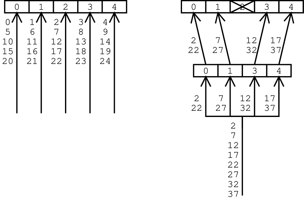
With the above rules, tasks assigned to functional items are not affected, while all tasks that would have to be processed by non-functional items are redistributed among the available ones. To show that in the case of errors the distribution is done evenly, a small test program has been written that simulates a number of item errors and fills histograms for each item with the number of tasks assigned to it. Sample distributions for a number of parameters are shown in Fig. 4.9.

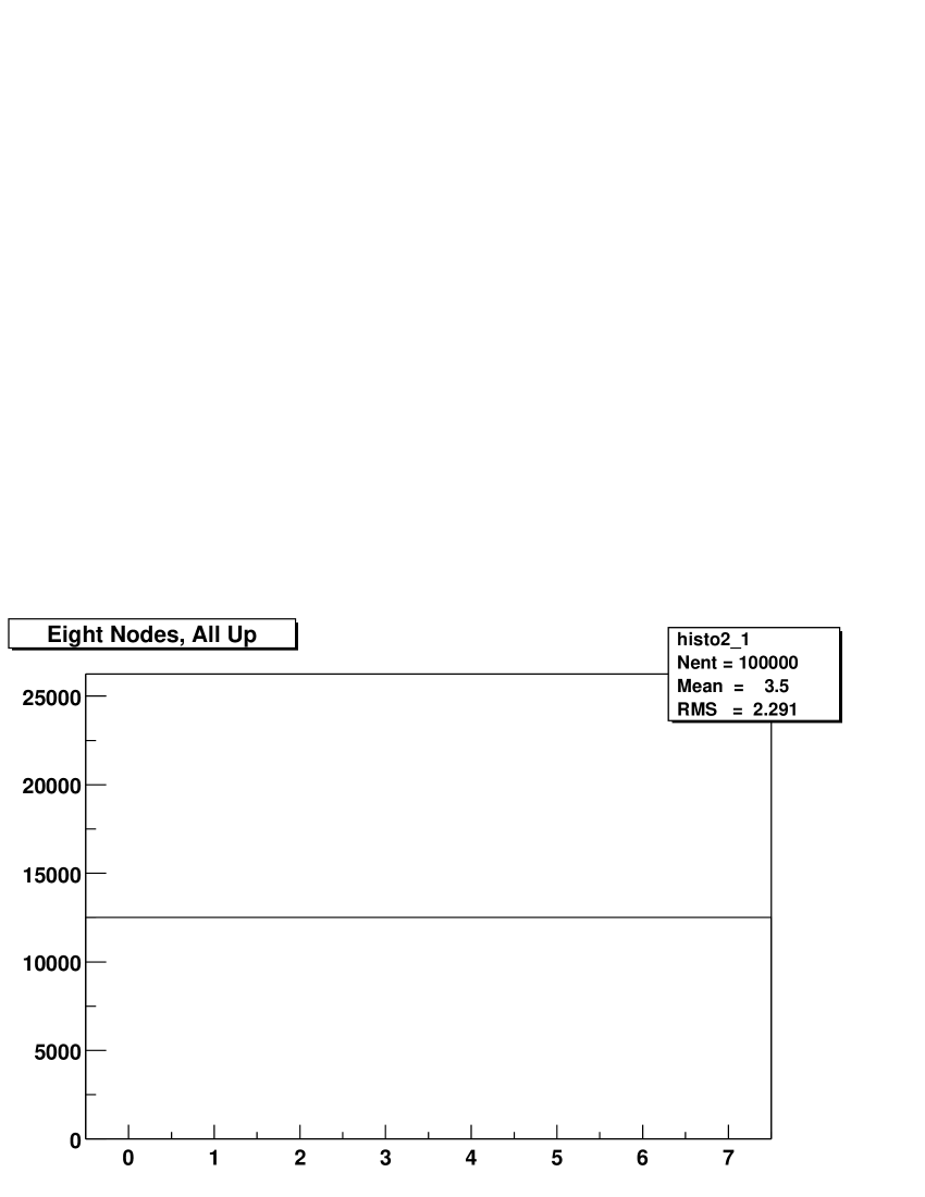

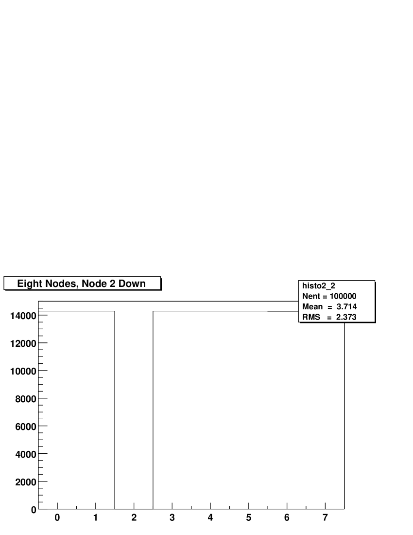
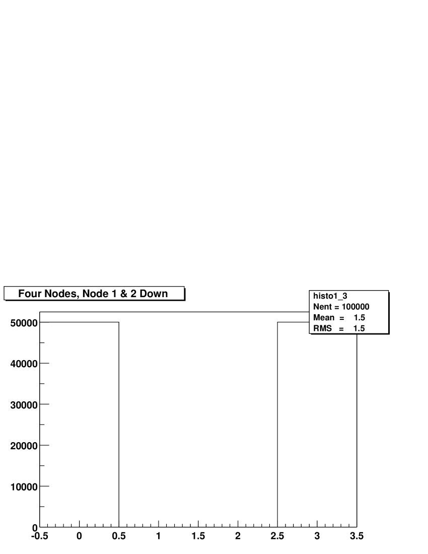
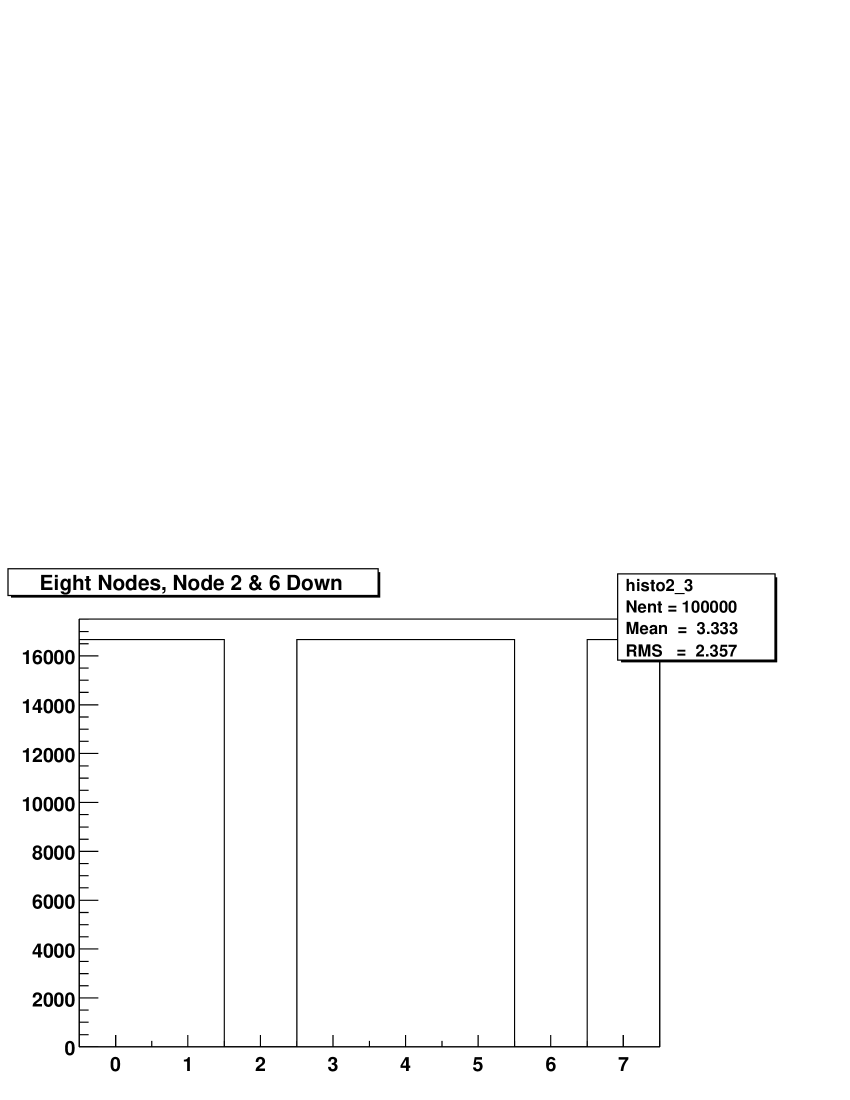
4.2.2 Functionality Replacement Classes
The MLUCVector Class
In the framework many uses of a dynamic array class involve an almost FIFO-like behaviour where new values are added to the end of an existing list. Access and removal of values, however, is not always strictly from the beginning but can in extreme cases be from the end as well. Typically though, removal is done from the first few elements of a list. Due to this non-strict removal from the head of the list, the queue class from the C++ Standard Template Library (STL) is not suitable, nor is any other queue class. A dynamic array class, allowing random access, is used instead. Although the STL list class is also usable in principle, tests have shown its performance to be slower than the vector class, probably because of the large number of element allocation and deallocation operations performed.
Unfortunately the STL vector class has a major drawback in this usage pattern. Whenever an element is removed all elements located after it in the list are shifted one slot forward. With a potentially very large number of events in the system coupled with a high rate this leads to a large number of copying operations that have to be executed in a node. For example, with event sizes of 8 kB, an event buffer size of 256 MB, an event descriptor size of 32 byte, and an event rate of 200 Hz, about 200 MB/s will be copied in memory just as a result of handling a list of event descriptors. To overcome this problem the new dynamic array class MLUCVector has been designed as a replacement class for the MLUC library.
Like the STL vector class the MLUCVector class is a template class with the template parameter defining the type of data stored. Unlike the STL class the MLUCVector uses a preallocated array as a ring buffer with a number of elements equal to a power of 2. In addition to the array for storing the contained elements themselves another array for a similar number of boolean elements is used to specify the validity of each element slot in the primary array. If the valid flag for a corresponding element slot is false, the slot is unused.
The advantage of using powers of 2 as sizes for a ring buffer is an easy wrap around handling. All operations on indices, e.g. the increment of an index for looping over all contents, are followed by applying a bitwise AND operation with a specific mask. This mask is the number of available elements minus one, corresponding to set bits for all valid indices in the buffer. Indices that have become too high or low by a previous operation are thus automatically truncated back to valid values. As the AND operation is typically very cheap, it often can be executed in one clock cycle by current processor types. It often is even cheaper to apply than to use the ordinary check for index wrap around. The combination of a comparison (or subtraction) operation coupled with a conditional jump that corresponds mostly to this check make these instructions typically at least as expensive as the AND operation applied in this class.
When an element is added to an MLUCVector object, it is inserted at the position specified by the end index of the ring buffer which is subsequently increased by one. In addition, the valid flag for that location is set to true, indicating that the slot is now used. For read accesses the index of a specific slot may be given, allowing random access to each element. To search for elements corresponding to specific criteria search functions are available that iterate over all valid elements using a caller supplied callback function for element comparison.
Removal of elements is done by specifying ring buffer indices, whose corresponding valid flags are then set to false. If the element to be freed is the first or last element, the appropriate index is increased or decreased respectively. When invalid elements are adjacent to such a freed boundary element the corresponding index is increased until a valid element is encountered.
When no free space remains between the ring buffer’s end and start indices two different actions are possible. If the ring buffer contains invalid elements, the buffer is compacted by shifting the valid elements together. After this operation the ring buffer consists of two separate blocks, containing all used and all unused element slots respectively. A buffer without invalid elements can be resized by doubling the size of its internal buffer arrays. Moving of elements can be necessary after a resize if the used element block wraps around the end of the buffer. In this case it has to be moved to the new end of the enlarged buffer. As soon as the number of used slots in a previously enlarged MLUCVector object drops to less than a quarter of the available slots the buffer is compacted again and its size is halfed. A buffer is never shrunk below its originally specified size. If resizing is not desired or necessary, then it is possible to set a flag in the constructor that inhibits resizing, both growing and shrinking, for the object concerned.
With the described features of the MLUCVector class it is ensured that the available resources, especially memory bandwidth, are used optimally for the dominant access pattern specified above. Correspondingly the change from the STL vector class to the MLUCVector class has brought a significant increase in the framework’s speed.
Allocation Cache Classes
To avoid copying large amounts of data, or small amounts very often, many parts of the framework only store pointers to data instead of the data itself. Only these pointers are passed between functions or different threads. This approach, however, has another problem of frequently issued allocation and deallocation calls, that usually are costly as well if used in such large numbers. In response to this problem two more classes, MLUCAllocCache and MLUCObjectCache, have been introduced into the MLUC library to prevent these frequent calls to the memory subsystem.
Both classes allocate a specified amount of elements on creation and store them in a pool of available elements. Instead of calling the normal memory allocation routines, e.g. malloc for C or new for C++, a program calls the allocation routine of one of these classes. This routine checks whether there is at least one element available in its pool and returns a pointer to the first available element if this is the case. The element’s pointer is then removed from the available pool and stored in a list of used elements. If the pool of preallocated elements is exhausted, the allocation objects use the system allocation routines to obtain the requested element. A pointer to this allocated element is stored in another list for additionally allocated elements.
When an element can be freed again the allocating object’s release function is called. If the element was allocated additionally, because the preallocated pool was exhausted, it is removed from the list it was stored in and is freed again, using the appropriate system deallocation call. For elements that originated from the preallocated pool, the pointer to the element is removed from the list of used elements. Subsequently it is reinserted into the pool to make it available for further use.
For both of these classes the amount of elements to preallocate is specified as a power of 2 and the MLUCVector class is used internally to store all element lists. The lists of available and used pool elements are both presized to the number of preallocated elements so that from the beginning both lists have enough space available to store all pool elements. No resize will be necessary for them. By using the MLUCVector class in this manner, the two classes benefit from its low overhead features and can handle operations on their internal lists efficiently.
The MLUCObjectCache class is a template class with the template parameter defining the type of elements for which the allocation object functions as a cache. Objects of the given type are preallocated, including executing their default constructor, and are stored in the allocation object’s pool. When a pool object is released again, it is not directly reinserted into the pool. Before the insertion one of its methods, ResetCachedObject, is called. This method’s task is to reset the object into a clean state, corresponding to its state immediately after creation, ensuring that a used object can be reused by the calling program without a check for a usable state. A consequence of this mechanism is that the ResetCachedObject method must be present in each class to be managed by an MLUCObjectCache instance.
In contrast the MLUCAllocation object manages only blocks of memory of a specified size. The block size is specified in the object’s constructor together with the amount of elements to be stored. Elements contained in an MLUCAllocation instance are neither explicitly overwritten with zeroes on creation nor upon release, again to save memory bandwidth. A program using an object of the MLUCAllocCache class thus can make no assumptions about the content of memory blocks received from it.
The String Class
Many pieces of code in the framework have to store a name or another type of textual information. Compared to the traditional C handling of the string type C++ string classes allow a significantly easier handling of these texts. In conjunction with the STL string class the discussed multi-threading of the framework poses a serious problem, as this class uses internal static members, globally shared between all objects of its type. Presumably for performance reasons these members furthermore are not protected by mutex semaphores. These global data items can thus be accessed and even changed simultaneously by multiple threads in a program. This behaviour has led to several very hard to trace bugs during the development of the framework until the real cause of the problem was found.
To work around the problem a primitive replacement string class, MLUCString, has been written and included in MLUC. This class is very simple, providing only the most basic functions to ease handling of textual data. Its function names also do not conform to the standard string class functions, as the aim was not to provide a complete reimplementation of the STL standard string class. Instead the decision was made for consistency reasons to have this string class conform to the naming conventions used in the MLUC class library as a whole.
Chapter 5 The Communication Class Library
5.1 Overview
One of the concepts of the ALICE High Level Trigger is to purchase the necessary components rather late, to take advantage of new technological developments. This concept should not only be applied to the cluster nodes themselves but to the network used for the interconnection of the nodes as well. To be able to support this aproach and, of equal importance, to maintain the generality of the framework, the communication technology and protocol used for communication between processes on different nodes have not been fixed. Instead a C++ class library has been developed that exports an abstract communication API with implementations for two network technologies. The API provided by this Basic Communication Library (BCL) has been designed to be generic and independent of any specific network technology. Despite this generality the API has also been designed so that implementations are able to make use of low-overhead, high performance, or efficiency capabilities present in the respective underlying network technology or protocol used. After evaluation the communication packages described in section 2.1 have not been considered as a basis for communication in the framework due to their different requirements, characteristics, and intended uses.
The API is split up into two parts, each optimized for a different communication pattern. Its first part is designed for the transfer of small amounts of data corresponding to the sending and receiving of short messages. For these small amounts of data the use of special transfer types like DMA is typically too much overhead so that they should be sent via Programmed I/O (PIO) transfers. The other API part is designed for the transfer of Binary Large OBjects (BLOBs), large blocks of data, in one transfer. For these block transfers any overhead needed for special transfers, e.g. DMA, is considered to be negligible compared to the actual transfer of the data. These special transfer mechanisms are thus acceptable and even desirable if they provide a lighter load on the host CPU and/or memory system.
To demonstrate the actual generality of the library’s API and also to provide a usable communication subsystem, two implementations providing the API’s functionality have been written. The first is based on the Transmission Control Protol (TCP) [22] as the most widespread network protocol. Its prime advantage is its availability on practically every computing platform and that most Unix variants, including Linux, contain a very robust and efficient implementation. For the hardware used with this protocol, Fast or Gigabit Ethernet are very widespread, with very cost-effective adapters being available for standard PC nodes. TCP’s disadvantage is its high overhead compared to dedicated System Area Network adapters, partly due to its design as a Wide Area Network (WAN) protocol over unreliable connections. The second communication implementation is provided, although only in a prototype form, for the SISCI API [126] on top of Dolphin SCI SAN [13], [90] interface cards. These SCI adapters are shared memory interface cards with a network bandwidth of more than 650 MB/s and latencies of below . Their primary disadvantages are the comparatively high price, which almost doubles the cost of a node compared to Gigabit Ethernet, and their weaker default reliability. Unlike TCP the SISCI API does not provide a reliable data delivery and packet loss has been observed although the physical layer specification guarantees packet delivery.
Various computers exchanging data can organize that data in different formats. The most common problem being the byte-order of stored multi-byte integer values. To avoid this type of problem when transporting data a number of helper classes and structures have been created that enable automatic translation of data between different storage formats. To take advantage of these capabilities the data types concerned have to be declared using a special type definition language. This language is then translated into normal C++ code by utility programs provided in the library.
5.2 Communication Paradigms
Several of the design decisions and paradigms chosen for the Basic Communication Library are different from design characteristics found in common network APIs, notably the socket API used for TCP. To avoid misunderstandings and confusion in later chapters these design decisions will be presented here.
5.2.1 General Design Features
A primary general design feature of the BCL library is that all data transport operations, both for message and block communications, can be executed with or without a previously established connection. In the library support is provided for establishing connections between two communication objects, but its use is not mandatory. If a data transport to a remote partner is performed without an explicitly established connection, then a connection will be set up implicitly for that transfer if required by the underlying protocol. After the transfer has completed the connection is terminated again. For a transfer to a remote partner, to which a connection is already established, this connection will be used to transport the data. The motivation behind this scheme is that in large systems it might be necessary to exchange messages with a large number of communication partners at a low rate. For these infrequent exchanges it would be too much overhead to establish open connections to all potential partners, if it would be possible at all and would not be restricted by the operating system. A user application should not be required to establish a connection manually for each of these transfers as that would complicate the application’s program unnecessarily. On the other hand, there may be frequent exchanges of data with other remote communication partners. For these the overhead of establishing a connection for each transfer has to be avoided, and a connection should be established only once. Therefore both explicitly as well as implicitly established connections are supported by the library.
One additional property supported for explicit connections is the on-demand connection. This means that a connection is not actually established immediately when the connection attempt is made. Instead the connection address is entered into an internal connection list but is marked as not yet established. When the first data transfer to this address is started, the connection is checked and found not to be established yet. As for an implicit connection, it is then established as part of the send operation. Unlike in the case of implicit connections, however, the connection remains established and is not terminated at the end of the operation. Like other explicitly established connections it has to be closed explicitly by the calling program as well when it is not needed anymore.
Another decision for the library is partially influenced by the above requirement for both connection-less and connection-based data transfers. Prior to any data send operation, each communication object must have been assigned its own receive address and must have performed a bind operation on it in order to make its address available to external programs. There are two reasons for this demand. The first of these, derived from the support for optional connections above, is that each program should be able to receive answers to messages it transmits. For the connection-less send mode the receiver cannot use the back-channel of a connection established from a remote object to it. In some instances sending of data requires a unique identifier in the system, e.g. to regulate access to a resource on a remote node. This remote identifier is trivially obtained by using a valid receive address for a specific network technology, which has to be unique by design. To ensure that a given address is actually valid and therefore unique a successful bind operation has to be performed on each communication object’s address before it can send data.
For some types of connections it might become necessary to perform some handshaking or negotiating before sending data even when using an already established connection. One example is SCI where multiple senders have to regulate access to a shared memory segment provided by a receiver process. Only in cases where a point-to-point connection is used between two communication partners, it is possible to avoid that overhead for each send operation. In these cases an already established connection can be locked and later unlocked by a sending object via two library functions. Locking of a connection makes the receiver object exclusively available to the locking sender object. No other sender object can send data to this receiver object even if a connection to it is established. This negotiation requirement is specific for ShM networks like SCI. Therefore the functions for locking and unlocking do not have to contain any functionality. A further function is provided so that an application program can determine whether a given communication object supports locking or not and can make use of the other functions as appropriate.
With regard to the handling of errors the choice has been made for a combination of return values and error callbacks. Every function in the library’s API returns an integer value of zero on success and a non-negative value describing the error that occured otherwise. These error values are taken from the standard C errno.h header file with the advantage that the preexisting C standard functions to convert the integer values to error descriptions can be used directly without any additional effort. In addition to these return values, that have to be evaluated explicitly, another method of detecting errors is available based on error callback objects registered with communication objects. The callback classes are derived from one common base class, that exports an interface of methods called for the various error types. If an error occurs inside a communication object it calls the appropriate function for all its registered callback objects. Parameters passed to these error callback methods include a pointer to the originating object and an integer value describing the error, identical to the error return value returned by the function. In addition to these two basic parameters further arguments are passed if necessary, e.g. the remote address for a failed connection attempt. After all callback objects have been called, the communication object’s function returns with the integer error described above. Exception handling has not been chosen for error handling to keep its use optional and not make it mandatory. It can be used by providing a callback object that throws an appropriate exception when one of its error functions is called. Beyond the callback objects registered statically with each communication object most of the communication objects’ function calls can accept an optional argument representing a pointer to an error callback object to be used in addition to the registered objects.
5.2.2 Message Communication Design Features
For the design of the message communication classes and their interface only a few design choices have been made. The primary design choice is to base the design on the pattern of sending and receiving of messages rather than on a stream of bytes, as e.g. for the standard socket API. Send and receive calls can include a timeout to be applied to the operation, which can be infinite. In most such cases, however, a fixed timeout of the underlying communication technology used, will expire and cause a system function to return with an error.
Another feature is actually more a requirement than a design decision. As a calling program cannot know in advance the size of a message received the allocation of the memory space for that message has to be made by a communication object’s receive method. By extension it also has to free the message again after the calling code has finished processing it, for which there are actually two reasons. The primary reason is that a calling program does not have to make any assumptions about the memory allocation function, e.g. new, new [], or malloc. Therefore the library has the liberty to choose which function to use and to change it without affecting a user’s program. The second reason is that for some network technologies it might be possible to store a message in an internal buffer which may even be done directly by the network hardware. The object then justs returns a pointer into that buffer without the steps of allocating memory and copying the message. Such a message is not freed using any system function but instead by the buffer management for the object’s internal buffer.
5.2.3 Blob Communication Design Features
For the blob communication mechanism more characteristics have been specified than for the message classes. Initially, a user may set the size of the buffer where received data will be stored so that user code can access it. For some of the blob communication implementations it may in addition be possible to specify the receive buffer itself. However, this feature might not be supported by a specific implementation of the blob interface, one example is the existing SCI implementation. Although it might not be possible to specify the receive buffer directly, a user always has the possibility to obtain a pointer to the receive buffer from the communication object. This enables it to write any received data into the receive buffer directly, from where it can be accessed by user programs. No additional copy step is required to copy the data from the communication object. Instead a user can directly access data that has been received from a remote node via the receive buffer pointer.
To enable this type of direct transfers it is necessary that the sending node knows beforehand where the data should be stored in the receive buffer and whether it is not already full so that the data cannot be stored at all. For this the sending process is split up into two parts each contained in its own function. In the first step an ID for the transfer is obtained by specifying the size of the data to be transferred. This transfer ID is queried from the remote receiving object, using an optional timeout, and then passed back to the user program. With this transfer ID the program can then use the second function by supplying it with the obtained ID and a pointer to the data to be sent. The communication object now has a receive buffer location associated with this transfer ID, and transfers the data to that location in the remote node. For this sending process a gather call is available where the data to be transferred is collected from multiple blocks scattered in memory. The size of data for which the transfer ID is obtained must of course be the sum of the sizes of all data blocks.
A transfer ID obtained for such a transfer is not automatically transmitted to the receiver object or program. Instead a user program has to pass it explicitly to its communication partner, most likely by using a message communication object. In the receiving program it is now possible to use the transmitted transfer ID to get access to the transferred data. Using the ID one can either obtain a direct pointer to the data or an offset to the data from the start of the receive buffer. With these informations a user program can access the data and process it as required. Once this is finished another communication object function has to be called to free the buffer block in which the data was stored. This block is again identified by passing the transfer ID used.
For the communication required between two blob objects, e.g. to negotiate a transfer ID, each blob communication object makes use of the facilities offered by the message communication mechanism instead of using an internal one. A message communication object is assigned to each blob object to be available exclusively to that blob object, implying that this message object must not be used by the user program. The advantage of this approach, besides avoiding duplicate development, is that the message communication may use another network technology than the blob communication. One example is if two technologies exist, one with low latency but comparably high overhead and the other with low overhead and higher latency. In such a case the high-overhead/low-latency technology could be used for the message exchange and the low-overhead/high-latency one for the blob transfers.
To achieve an even lower overhead of sending with the avoidance of the additional latency incurred by the negotiation phase before each transfer a special approach can be taken. A sender can allocate a large block of a remote buffer in advance by requesting a large transfer block. This block could be as large as the whole buffer which is made possible by using a function that queries a remote node’s receive buffer size. The transfer ID of this block is sent once to the remote object, which stores it for future use. From this point on the sending program can perform a completely local buffer management in its obtained block and only sends the offsets in that buffer to its receiving node. This completely avoids waiting for reply messages from the receiver and decreases the time overhead associated with each data transfer by twice the message sending latency.
5.3 Auxiliary Classes
5.3.1 Data Format Translation
One of the main problems encountered in network communication on potentially heterogeneous systems is the different format of stored data, most often encountered in the form of different byte orders for integer data. To work around this problem, a helper hierarchy with one base class and structure is included in the BCL. The base structure, BCLNetworkDataStruct, provides a header for derived data to be stored. Derived types are used to actually store the data. Code and meta-data required to execute the translations is contained in the base class as well as its derived classes. In the header three elements are stored to provide information about a structure’s original data format at creation, its current data format, and the total length of the data structure. Since the native data format of any given system node is trivially known it is always possible to convert data, described by this format, into a node’s native format. By also supplying the data’s original format, it becomes possible to handle data not directly under the control of this mechanism as well. This cannot be done automatically anymore though. Including the total length of the structure furthermore enables all software stages to know how much data they have to handle without having to know its actual content.
In the basic class BCLNetworkData a number of static member functions are provided to transform integer data of different sizes between data formats. For each of the integer sizes 16 bit, 32 bit, and 64 bit two functions are available to convert the data. One can be used to convert the data in place. The other one works with separate source and destination, copying the data during the translation process. In addition to these static functions, the class provides further functions to aid the handling of different formats of data. Importing of data structures into a class is supported by different methods either at an object’s creation using its constructor or by calling member functions later. At creation only two possibilities for copying the data into the class’s internal data structure exist: transforming it to the node’s local format in the process or copying the data untransformed. For an existing object it is possible either to copy the data structure, as on creation, or to adopt it by setting an internal pointer to the structure. Both approaches can optionally be combined with the same data transformation possible for the constructor. The advantage of the second approach is that it avoids the overhead of copying data, which for large amounts of data and/or high frequencies of transforming data can be quite significant. After data from a network data structure has been imported into an object, functions exist, that allow to transform the data, either to its original format, the node’s current format, or a user specified data format. In addition it is possible to query both the data’s original as well as its current data format.
Data types to be managed by this mechanism have to be declared using a very simple type definition language (vstdl), translated into normal C++ code by a program in the BCL library. The language supports only plain 8, 16, 32, and 64 bit sized unsigned integer types. Each structure type must be derived from another vstdl type, at least from BCLNetworkData, as its two respective C++ elements contain the translation functionality. A sample of the declaration of such a datatype is given in Fig. 5.1, showing the three size options available for a structure element: A single scalar type, a fixed size array, or a variable size array. Fig. 5.2 shows the C++ structure type generated from the previous vstdl definition. As for the base BCLNetworkData types the generated class and structure differ by the Struct modifier appended to the structure’s name. The base name for both is the name specified in the vstdl type definition and both are derived from the corresponding C++ type for the vstdl parent type. Transformation is performed in the inverse inheritance hierarchy. A derived class first converts its own elements and then calls its parent class’s transformation functions.
Structure elements of the variable size array type can only be contained as the last element in a structure. Otherwise the C++ declaration of the structure would have to allow moving subsequent elements due to the array’s changing size, this however is not supported by the C++ language. This also implies that each structure can only contain one such element. For these elements the array is preceeded by an automatically generated member, holding the number of actual elements making up the array, to allow for the correct handling of the changing array size.
#// Anything after a ’#’ at the beginning of the line is copied #// verbatim into the generated files. # name SampleData: BCLNetworkData uint32 fField; uint8 fArray[4]; uint16 fVarArray[]; #
// Anything after a ’#’ at the beginning of the line is copied
// verbatim into the generated files.
struct SampleDataStruct: public BCLNetworkDataStruct
{
uint32 fField;
uint8 fArray[4];
uint32 fVarArrayCnt;
uint16 fVarArray[0];
}
A sample hierarchy of three generated vstdl data types from the BCL is shown in Fig. 5.3, with the vstdl types on the left side, the generated C++ classes in the middle and the generated C++ structures on the right. The vstdl BCLNetworkData type displayed in the figure exists only virtually, since only C++ class and structure exist for the represented base type. Of the three vstdl types BCLAbstrAddress and BCLMessage are directly derived from BCLNetworkData while the third type, BCLTCPAddress, is in turn derived from BCLAbstrAddress. In the resulting C++ classes and structures the hierarchy of the respective vstdl types is reflected directly. Also displayed in the figure is the mutual dependency of each type’s class and structure with the class directly containing an embedded structure type as well as a pointer to the structure. This pointer is used to access structures that have not been copied into a class object but that have been adopted for efficiency reasons as discussed.
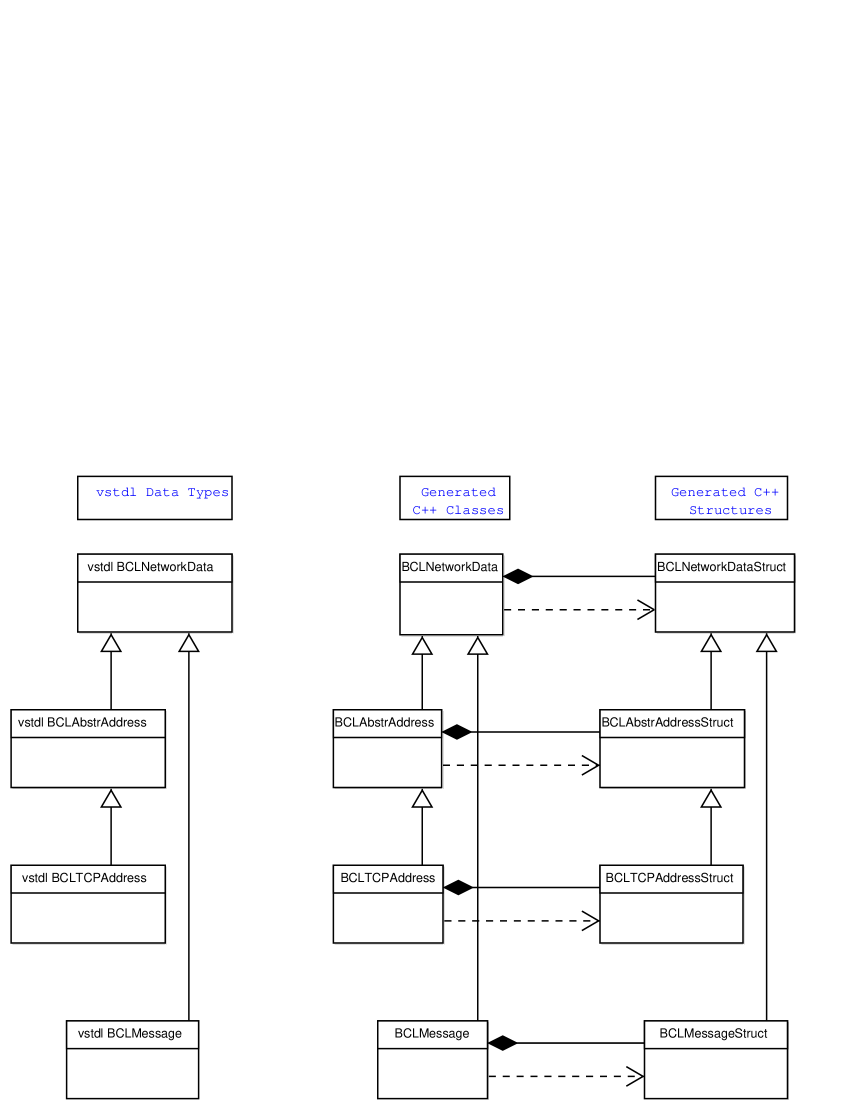
Using the interface provided by BCLNetworkData and generated classes for other vstdl data types, it becomes possible for programs to handle the parts of data it needs, independent of the data format they were originally stored in. This is achieved without having to write the conversion code for every data type explicitly, which can instead be written as a vstdl type definition, from which the necessary C++ code is subsequently generated. One drawback of the mechanism employed is that code working with C++ types generated from a vstdl data type definition is unable to transparently handle derived data types as well. It will always handle only the data elements it was compiled for. A more mature and flexible data format conversion scheme might be implemented and used in later versions of the library and framework.
5.3.2 Address Classes
Addresses used in the BCL library are based on a vstdl type hierarchy, with the abstract address type BCLAbstrAddress at its root. BCLAbstrAddress is shown in Fig. 5.3. It contains only an integer element that defines the type of address in addition to the BCLNetworkData inherited header. Each communication implementation defines its own constant to identify its address type, e.g. 1 for SCI and 2 for TCP. The address types for each network technology are derived from the BCLAbstrAddress type, included are implementations of addresses for SCI as well as for TCP.
SCI addresses include three 16 bit elements, the first of which is used to identify the specific node concerned. It is unique to each SCI adapter card, making it rather an adapter than a node ID but is sufficient to identify a node. Which adapter in a node is used for transmission is defined by the second number in the structure, this number is required if multiple adapters are present in a node and is 0 otherwise. The third number finally holds the ID of the shared memory segment used to receive the data in the target node and must be a unique identifier in each node. For TCP the address structure contains only two elements, a 32 bit field with the target node’s IP number and a 16 bit number for the port that the receiving communication object uses. Fig. 5.4 shows the three different vstdl types used for address handling. At the top is the abstract address type definition with its single element to define the network technology supported. In the middle is the SCI address type with its three described 16 bit numbers, and at the bottom the TCP address with the IP and port number required for a TCP connection.
name BCLAbstrAddress: BCLNetworkData uint32 fComID; name BCLSCIAddress: BCLAbstrAddress uint16 fNodeID; uint16 fAdapterNr; uint16 fSegmentID; name BCLTCPAddress: BCLAbstrAddress uint32 fIPNr; uint16 fPortNr;
5.3.3 Message Classes
For the message communication mechanism the basic datatype used to define the message header, BCLMessage, is derived from BCLNetworkData. It is thus also based on the data transformation mechanism from section 5.3.1. The first of its three fields contains an ID that defines the type of the message, outside the scope of the library and under the control of the application. Unlike this field the second field contains an ID to identify messages, reserved for use by the library itself. For the current implementations this is just a counter increased for each message sent. The final field allows the specification of flags to affect the sending of a message. At the moment, though, the field is not used by the library and no flags are specified, neither general message flags nor flags specific to an implementation of the message communication interface. Fig. 5.5 shows the vstdl type definition of the BCLMessage type with the three fields described.
name BCLMessage: BCLNetworkData uint32 fMsgType; BCLMessageID fMsgID; uint32 fFlags;
5.3.4 Error Callbacks
Error handling is performed partly by a set of callback object classes derived from the abstract base class BCLErrorCallback shown in Fig. 5.6. Instances of this or derived classes can be registered with communication objects and provide a number of callback functions, called by a communication object when the corresponding error has occured.
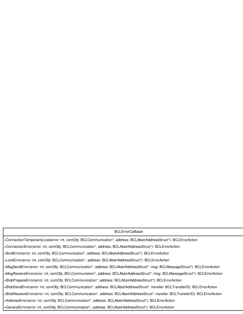
As can be in seen in Fig. 5.6, the class contains callback methods for different types of errors:
-
•
General errors, applying to any communication object
-
•
Send and receive errors for message communication objects
-
•
Prepare, send, and receive errors for blob communication objects
All methods accept at least a set of three common parameters: an indicator for the error that occured, a pointer to the originating communication object, and a pointer to an address structure involved. Depending on the context this last parameter may contain either a local address, e.g. on a bind operation, or a remote address, e.g. for a connect or send operation. In addition to these common parameters more may be accepted or required as appropriate for the error type that occured. For message errors this is a pointer to the message concerned by the respective error and for blob transfers it is the transfer ID. The available callback methods are not declared as abstract methods. Instead each is provided as a default implementation that only returns a default value described below so that derived classes have to implement only those methods whose functionality is needed.
The value returned by the callback functions is an action indicator containing a suggestion from the callback object how to handle the error. This action can have one of three values indicating either to ignore the error, abort the operation, or make a retry attempt of the failed operation. Since the value is only treated as a suggestion the communication object can ignore the values returned by all callback objects and proceed differently, as an action might not be possible for a specific case. In the current implementation of the communication classes, the error callbacks’ return values are not evaluated at all, but the option to do so is already present for later implementations of the library.
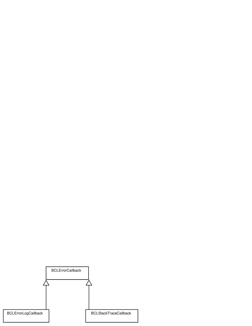
Next to the base callback class two more derived classes are contained in the communication library, shown in Fig. 5.7. The first of these, BCLErrorLogCallback, calls the logging system of the MLUC library with an appropriate error message constructed from its parameters. In the other class, BCLStackTraceCallback, a set of system debugging functions is used to dynamically obtain a trace of the current call stack. This trace is then also passed to the MLUC logging classes. Beyond these two included classes an application can also derive its own classes from BCLErrorCallback to implement any error callback handling necessary.
5.3.5 Address URL Functions
To support future additions of communication classes to the library without the need to recompile programs using the library, a set of functions is included in the library that allows to specify BCL communication addresses in a Uniform Resource Locator (URL) like format. Addresses in this format specify the network technology to be used, whether the message or blob communication mechanism is to be used, and the specific address information required by the technology concerned. In this way a generic separation of address handling and network technology has been introduced into the library. The supported abstract address format supported is now essentially a string type. Fig. 5.8 shows the syntax for TCP and SCI addresses. As can be seen in the figure, the elements of the URL specifying the actual address correspond to the elements of the respective address structure types described in section 5.3.2.
tcp(msg|blob)://<IP Nr>:<Port Nr>/ sci(msg|blob)://<SCI Node ID>[.<Adapter-Nr>]:<Segment ID>/
Address URLs are processed by four functions in the library, two for creating BCL objects and two for releasing them. Objects can be allocated for either local or remote addresses by the BCLDecodeLocalURL or BCLDecodeRemoteURL function respectively. For local addresses an address structure is returned together with an appropriate communication object of a class derived from BCLCommunication. Additionally, a flag is provided indicating whether the returned object is a message or blob communication object. To release allocated objects two BCLFreeAddress functions are available, one to release only an address structure and the second one to also release the communication object. A fifth helper function, BCLGetAllowedURLs, is provided to aid in providing lists of allowed addresses to program users. It returns two list of strings containing valid message and blob address URL formats.
5.4 Communication Classes
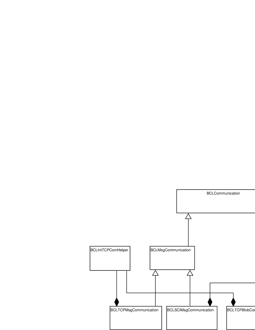
The seven primary communication classes in the library are organized in a tree hierarchy, displayed in Fig. 5.9. At the root of this class hierarchy is the BCLCommunication class, providing basic services and declaring interface functions common to both of the previously described communication types. Derived from this class are BCLMsgCommunication and BCLBlobCommunication, which declare interfaces and implement common services for the message-like and data-block communication mechanisms respectively.
Two classes are derived from each of the two communication type base classes to provide implementations for the TCP protocol using the standard socket API as well as for the shared memory interconnection technology SCI by Dolphin using the SISCI API. All four implementation classes are designed to be able to make use of as many performance and efficiency optimizing features as possible for the specific network technology used. In addition to these primary communication classes two separate classes, BCLIntTCPComHelper and BCLIntSCIComHelper, are present, used by the two implementation classes for each network type as shown. They supply functions and variables common to both communication mechanisms but specific to each network technology. These two classes are not intended to be used directly in a program but are for the library’s internal use only as signified by the Int specifier in their names.
5.4.1 The Basic Interface Classes
The BCLCommunication Class
At the base of the communication class hierarchy is the BCLCommunication class containing functionality common to all communication types and mechanisms. Primarily, however, it defines the common interface for the different communication types using abstract member functions. A UML diagram of the class with the main features described in the following paragraphs is shown in Fig. 5.10. The main functionality contained in BCLCommunication is the handling of the error callback objects, that can be registered with each communication object. Two public functions are provided, allowing to add or remove callbacks to a communication object plus a number of protected methods for internal use by this or derived classes. Each of these functions corresponds to one of the different error functions exported by the callback interface. They are called when an error occurs and in turn call the appriopriate error function for each registered callback object as well as for the optional callback parameter object supported by most functions.
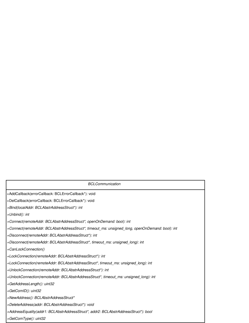
Common interface parts defined by the BCLCommunication class include functions for binding, connecting, locking connections, handling addresses, and one function for querying whether a communication object is a message or a blob communication object. For all functions any address needed must be specified in the form of a base address structure BCLAbstrAddressStruct or a pointer to it, to keep the interface generic from a specific network technology. The actual address used still has to be of the type required by the corresponding communication object itself and is thus specific to the network technology supported by that object.
The Bind function defined in the interface requires one argument only, a structure pointer holding the address to which the communication object should be bound. Data sent to this address must be received by the communication object, and the address therefore must be a valid address for the network technology chosen. No parameter is required by the Unbind function, which releases a bind to an address, as each communication object has exactly one address it is bound to. Both functions return an integer value to indicate the success or error status of the operation as described previously. Unlike the Bind call the Connect call exists in two versions: one using a millisecond granularity timeout value and the other without a timeout. Both calls require a remote address to connect to and a boolean stating whether the connection should be established immediately or as an on-demand type connection, as explained in section 5.2.1. The supplied default value of false for the boolean parameter specifies that the connection has to be established immediately. As a communication object can be connected to multiple remote communication partners the Disconnect function requires the remote address of the connection to be terminated. Similar to the Connect function, the Disconnect function also exists in two variants, one with a milliseconds timeout and one without. All four connection related functions return the standard integer error indicator.
The following set of five functions is responsible for locking connections, with the first of these functions allowing to query whether the locking feature is supported by this object, which depends on the network technology implemented. Two functions are available to lock an established connection, one with timeout value and one without. Like the Connect function both need the address of the remote connection partner and return an integer error value. The two unlock functions are also similar with respect to their required arguments. Each needs the address and one of them allows to use a timeout value.
Support for handling network addresses in an abstract manner is provided by the final set of functions defined by BCLCommunication. In conjunction with the set of helper functions that allow to specify addresses in a string similar to Internet address URLs, any user program working with address classes needs to know as little as possible about the format of the underlying addresses and the specifics of the network technology used by a communication object. The first two of the address support functions allow to query two values relevant for address handling, namely the actual length of an address and the value of the communication ID. These two values allow to identify whether a given address belongs to a specific communication implementation. The address length is also required for storing, copying, or allocating addresses.
Allocating memory for addresses is also supported by the second set of two functions, that allow to allocate memory for an address and to free an allocated address. The allocation function NewAddress returns an address structure object with header fields and the communication ID initialized to values appropriate for the communication object. DeleteAddress frees the memory allocated for an address structure by using the free call corresponding to the allocation call used in NewAddress. By using these two functions it is ensured, that the allocate and free functions always match, the correct amount of memory is allocated, and the basic fields are initialized correctly. A fifth address helper function is used to compare address structures for identity, to support comparing of addresses whose exact type and contents might not be known at compile time. Comparing two structures bytewise relying on their length is always possible, but addresses with different byte contents might point to the same remote address, e.g. because of different byte orders. The final helper function provided by BCLCommunication specifies whether a communication object is a message or a blob communication object so that it is possible to distinguish between these two sub-hierarchies in a generic manner.
The BCLMsgCommunication Class
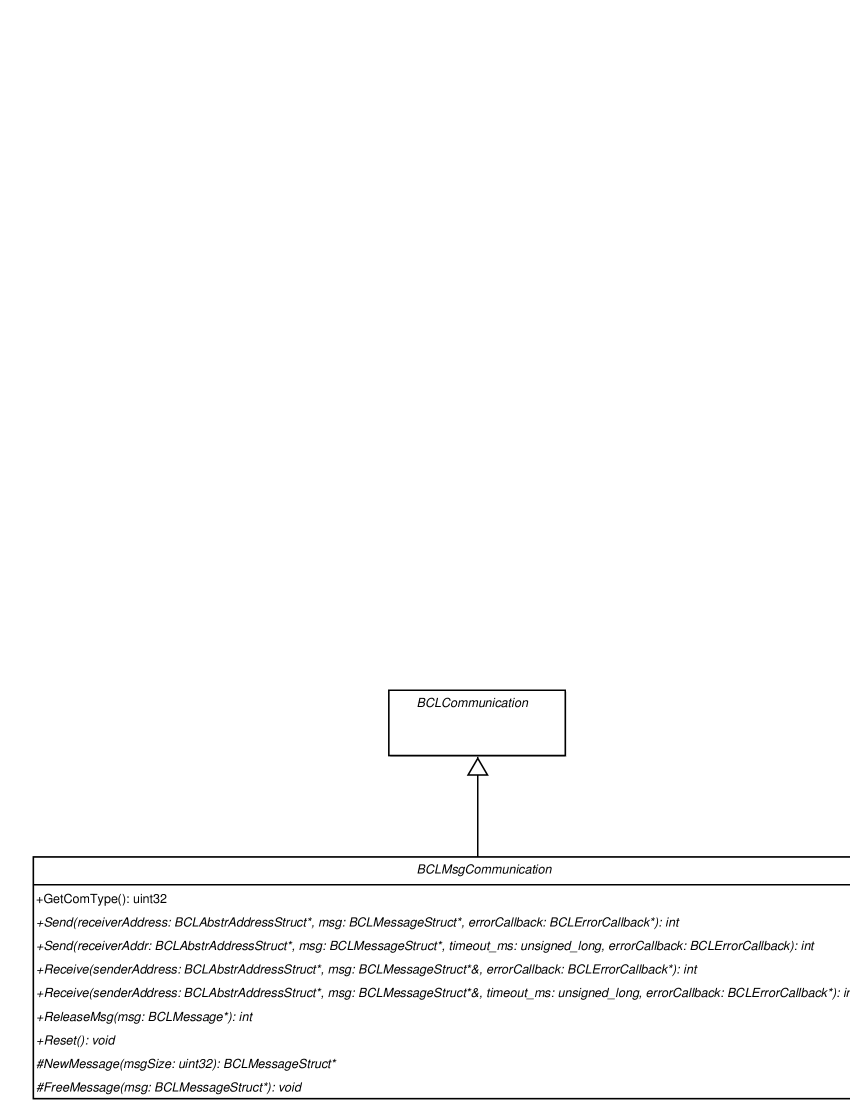
The BCLMsgCommunication class is derived from BCLCommunication. It defines the interface for the message communication mechanism, as shown in Fig. 5.11. This class provides almost no additional functionality beyond that provided by BCLCommunication but defines the interface only. The one supplied functionality is the implementation of the helper function to distinguish between message and blob classes, which returns the indicator for a message communication object so that derived classes for specific network technologies do not have to implement this function themselves. Primarily, the BCLMsgCommunication class defines the interfaces for sending and receiving of messages on top of the basic interface defined in BCLCommunication. Beyond these send and receive calls a Reset call is provided, that serves to reset a message communication object to a clean defined state. Resetting an object might cause some previously received data to be lost.
For all Send functions two parameters are needed, the remote address where to send the message to and the message itself. The address is supplied as a pointer to a BCLAbstrAddressStruct object, and the message is specified as a pointer to a BCLMessageStruct structure. This message object can be of the actual BCLMessageStruct type, or it can be of a structure type derived either directly or indirectly from BCLMessageStruct. An optional third respectively fourth parameter is a pointer to a BCLErrorCallback object. In the case of an error this object’s error reporting callback functions will be called prior to those of the communication object. In order to always provide a Receive function with a message’s originating address, a Send function implementation should send its address prior to the actual message data. This might not be necessary, if the remote communication partner has other methods of finding out the originating address of a received message, but a Receive function must always be able to provide a message’s source address.
The Receive functions also accept two mandatory and one or two optional arguments. In analogy to the Send functions the Receive function’s optional parameter is a callback object whose functions will be called in addition to the ones of registered objects. As their first parameter, both Receive functions use a pointer to a memory location where the address of the sending communication object will be stored. A check is executed whether the structure has the correct length expected for addresses used by this communication object. If that size is incorrect, the Receive call fails. The second mandatory parameter is a reference to a BCLMessageStruct pointer, used to return the received message itself to the calling program. Memory to store a message is allocated by a call to NewMessage, another function provided as the declaration for an abstract member function, to be implemented by derived message communication classes. The function is declared as a protected member function so that it is only available for internal use by other methods of this or derived classes and not as an interface to programs. Allocated memory for a message is filled with the contents of the message received. The pointer to the new message is returned via the reference parameter. It is not mandatory for the Receive calls to allocate memory for the message data, it could for example also be stored in an internal buffer, or it might be written directly into a reserved buffer by the sender, like in the case of SCI. Here it would be sufficient to return a pointer to this internal buffer memory.
A message that has been received and its memory been allocated, has to be released again after the program has finished using the message’s data. To retain flexibility in the way the messages are allocated in the Receive functions, the BCLMsgCommunication class declares the ReleaseMsg method for this purpose. It accepts a pointer to an allocated message as its argument. This pointer is then passed to the protected member function, FreeMessage. As is the case for NewMessage, FreeMessage is also declared as a pure virtual member function to be implemented by derived message classes.
The BCLBlobCommunication Class
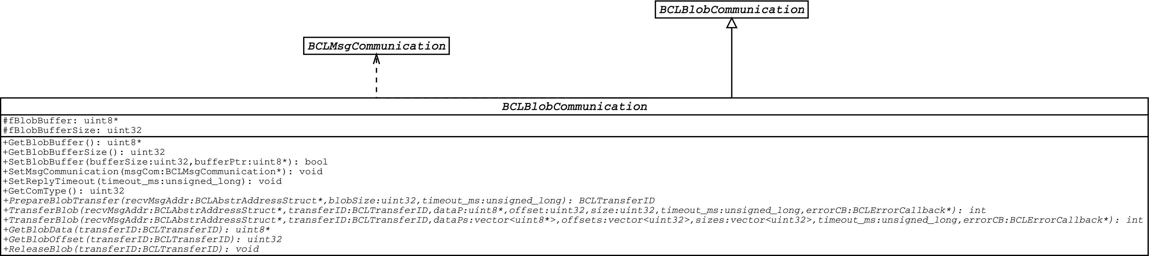
As the BCLMsgCommunication class, the BCLBlobCommunication class shown in Fig. 5.12 is also derived from the BCLCommunication class. It contains functionality for the blob communication mechanism and also declares an abstract interface for it. Functionality is provided by this class mainly for the blob receive buffer, that stores data received from remote nodes for access by the program. One further helper function in the class is an implementation of the function from the BCLCommunication class that identifies objects of this and any derived class as blob objects. The main function for the receive buffer is used to specify the buffer’s size and optionally the receive buffer directly by using a pointer to the respective area of memory. Setting the buffer’s size is always allowed, it is allocated immediately with the new size. If the buffer was already allocated, the old buffer is released and a new one allocated with the given size. Specifying the buffer to be used itself in a parameter to this function is not guaranteed to be supported. This depends on the blob implementation. For the SCI implementation, for example, this is not possible, since received data is written directly into the buffer by the remote sender program. As the current implementation of the SISCI API for SCI does not allow to specify arbitrary memory locations into which data can be written remotely, the allocation of the receive buffer has to be done by the SISCI driver or library. To allow the required overriding of the original SetBlobBuffer function in BCLBlobCommunication by blob implementation classes the function is declared as a virtual function. Two additional helper functions are available to obtain a pointer to the buffer for accessing received data and to query the buffer’s size.
As was pointed out in section 5.2.3, the blob communication mechanism has to exchange handshaking and control messages with a remote communication partner using exclusively reserved message communication objects. The specification of the message object to be used by a blob object can be done either in a BCLBlobCommunication constructor or it can be done later using a separate function. Both approaches use a pointer to the message object set in the blob object. A helper function allows to set the timeout used to wait for answers from the remote node via the associated message communication objects. When replies are not received within the specified timeout they are treated as errors. An exception is the special timeout value of 0 which disables timeouts, resulting in an infinite wait.
The blob communication interface, declared by the BCLBlobCommunication class, consists of two parts, the interface for the sender to transmit the data and the one for the receiver to access received data. Each of the declared sending and receiving interfaces consists of three pure virtual functions. Before a transfer is started, a negotiation has to be performed first to determine where to store the data in the receiving buffer, if it can be stored at all. This negotiation is performed by the PrepareBlobTransfer function, that uses the address of the remote message communication object associated with the receiving blob object. It is not necessary for the object to know the address of the blob object itself. The second parameter required by this function is the size of the data to be sent, the data itself is not passed to the blob object for the preparation of the transfer. Optionally, a timeout can be supplied as well, in order to restrict the time that the function waits for the reply from the remote message communication object. On a successful negotation the function returns an ID that can be used subsequently to execute the transfer. Using the returned transfer ID the data can be sent to the remote blob object with the help of one of the two available TransferBlob functions. Both functions require the remote message address as their first argument followed by the transfer ID returned from PrepareBlobTransfer. Two optional arguments, supported by both functions, are a timeout and a pointer to an additional error callback object. This object is used in addition to the registered callback objects. By default the timeout is disabled through the value zero and the default callback pointer is empty.
In addition to these common parameters the simpler of the two transfer functions accepts three more parameters that describe the data to be transmitted. Of these parameters the first is a pointer to the actual data to be transmitted itself, followed by an offset holding the location where this data block should be stored in the previously reserved receive transfer area. The offset is specified relative to the start of the reserved transfer area and can be used to write multiple data blocks into a transfer area with multiple calls. This is needed especially when a larger portion of the receive buffer is reserved in advance, and the sender performs its own buffer management in that area, as discussed in section 5.2.3. As the function’s final parameter, the data size is specified. The sum of the size and the data offset must not exceed the size parameter passed in the transfer preparation function call. Explicitly specifying the size parameter is done to allow splitting a transfer over multiple calls in conjunction with the function’s offset parameter. Unlike the first transfer call, the more complex second one allows to perform a scatter-gather-transfer with one call. Therefore the three parameters describing the transfer, data pointers, offsets in the receive buffer, and block sizes, are not specified as scalars but instead as three vectors, or dynamic arrays, each containing multiple values. The arrays holding the pointers to the data and data block sizes must contain the same number of elements for the transfer attempt to be valid, but the array of offsets can contain less values than the other two arrays and may even be completely empty. If it contains less offsets than needed, the remaining offsets will be calculated so that each block will be immediately adjacent to the previous block. In particular this means that if no offsets are specified the blocks will start at the beginning of the transfer area and will then continue directly adjacent to form a single large block. Essentially this provides a merging or coalescing functionality for the scatter-gather-transfer.
Three functions make up the receiving interface of the class, each of which uses only one parameter, the ID of a received transfer. One of the functions, GetBlobData, returns a pointer to the beginning of the area of the receive buffer. With this pointer an application program can access the data that was received for the particular transfer. GetBlobOffset, the second function, returns the offset to the transfer’s block in the buffer, relative to the buffer’s start. Together with the pointer to the receive buffer itself this can also be used to get access to the received data. The final receive interface function, ReleaseBlob, is used to release the buffer space occupied by a received transfer. No method is provided by the blob communication interface to send a transfer ID to a receiving node or to wait for a completed transfer. This has to be done explicitly by a user program, for example using a second message communication object.
5.4.2 The TCP Communication Classes
The classes presented in this section implement the message and blob facilities on top of the widely used Transmission Control Protocol (TCP) [22]. Both primary classes BCLTCPMsgCommunication and BCLTCPBlobCommunication for the two different communication mechanisms make use of the services provided by a third class, BCLIntTCPComHelper. Communication is based upon the established POSIX socket API [119], [120], [121], [127], available on basically every Unix system as well as on Windows systems. TCP is a connection-oriented protocol, and the use of the BCL communication functions without an explicitly established connection results in a TCP connection being initiated for the duration of the sending. On the other hand, the system API used to access the TCP protocol trivially allows to receive data from multiple connections simultaneously, making the locking functionality unnecessary for TCP.
The TCP Communication Helper Class
In the BCLIntTCPComHelper class functions are provided for the TCP protocol used by both communication mechanisms, and which therefore have been placed in a separate class for reuse. Most of the functions supplied by the TCP helper class follow the interface defined by the top-level communication class BCLCommunication and differ primarily in the number and type of parameters. Parameters supported by this class can be made more specific for the TCP implementation compared to the generic interface definition. For example, for the functionality to bind to a valid address provided by the helper class’s Bind function, the generic address pointer to a BCLAbstrAddressStruct instance is replaced by a BCLTCPAddressStruct pointer.
In the Bind function the socket that will be used to accept incoming connections is created using the socket function. The SO_REUSEADDR flag is set by the setsockopt function to allow the socket to bind to an address that has been in use before and not been properly cleaned up. Since a bind to an address in actual use will still fail, the option can be safely used here. After setting the flag the socket is bound to the port number from the specified address using the bind API function. If an IP number has been specified in the address the socket will be bound to that particular address so that data can be received only from the network interface associated with that address. Otherwise it will not be bound to a particular IP number, and data sent to any IP address of the current node can be received. When the bind call has completed successfully, the socket is set to a state in which the system accepts incoming connections using the listen system call. Finally, a background thread is created to wait for and handle incoming connections as well as data arriving on an already established connection. This accept thread is described in more detail below. Analogous to the Bind function the helper class also contains an Unbind function that ends the ability to accept incoming connections and data. To unbind the socket created above the function sets an internal flag and tries to establish a short connection to the local receive socket itself to activate the created accept thread. Upon activation the thread checks whether the flag has been set. If this is the case, it cleans up and terminates, setting another flag in the process. The connection established by the Unbind function is closed again immediately, and the function waits a specific time for the second flag to be set, signalling the termination of the accept thread. If the flag is not set within the required timespan the thread is aborted forcefully. After termination or abortion of the accept thread, the accept socket created in Bind is closed to complete the unbind operation.
The second type of functionality provided by the TCP helper class for both communication mechanisms is the ability to connect to and disconnect from remote communication objects. For this purpose two interfaces are available in the helper class. One of these interfaces is identical to the connection interface supplied by the BCLCommunication class, again with the exception of TCP address structures being used instead of abstract addresses. Its parameters are the address pointer mentioned, a flag whether a timeout is to be used together with the timeout value, and a boolean flag specifying the connection type. The timeout value may be ignored depending on the timeout flag’s value and the connection flag indicates whether to connect immediately or create an on-demand connection. This interface is used for explicitly initiated connects by the TCP communication classes. It makes use of the second basic connection interface in the helper class.
This second helper connection interface is used by any sending function in the TCP communication classes that needs to use a connection for the duration of the send operation as well as by the explicit connection interface. The function for initiating a connection, ConnectToRemote, requires as its primary arguments a pointer to the TCP address of the remote connection partner and a pointer to a structure used internally to store data for an established connection. In this structure the remote address and the socket used for this connection are stored together with a use count. It is filled by the connection function and allows the code that initiated the connection to use it through the stored socket descriptor. In addition to these arguments ConnectToRemote supports two more input flags and one output flag, the first of which specifies whether the connection should be established immediately or as an on-demand connection. The second input flag controls whether the connection is a permanent connection initiated by an explicit user connection call or whether it is an implicitly established connection. In the first case, the connection data as returned by the function is stored in a list of connections if it has not been stored there already. Related to this, the output flag of the function indicates whether the connection was already stored in the connection list, indicating that the connection had already been established before the ConnectToRemote function call.
If the connection has been already established, only its data is copied into the connection data structure, and the appropriate output flag is set so that a connection can be used multiple times. For a connection that needs to be established immediately, but that has been stored as an on-demand connection, the call will cause the connection to be established. The established connection’s data will be stored in the slot already used. It is stored independently of whether the function call causing the connection to be established, specifies a permanent connection or not. When a connection cannot be found in the internal connection list three possibilities have to be distinguished.
-
1.
An on-demand connection that has to be stored: In this case just the remote address is stored in the list with a usage count of one and an invalid socket descriptor. The invalid descriptor indicates later calls to this function that the entry is an on-demand connection which still has to be established.
-
2.
An immediate connection to be made permanent as well: In this case the connection is established as described below and, if successful, stored in the internal list.
-
3.
An implicit connection from a transmission operation: This connection needs to be established immediately but does not have to be stored in the internal list. It is also established as described below, but contrary to the other cases the connection data is only returned to the caller and is not placed in the list.
If a connection has to be established for one of the three cases listed above, certain steps are executed in ConnectToRemote, starting with the creation of the socket used as the local endpoint for the connection concerned. After creation the TCP_NODELAY socket option is set as any message should be sent immediately without waiting for further data that might have to be sent. When these preparation steps are completed an attempt is made to establish the connection using the connect system call. If a timeout has been specified, it is used for the connection attempt by setting the timeout with the SO_SNDTIMEO socket option. After the connect function returns the old timeout value is restored. At this point the connection has been established if the connect function signals success and the connection data can be stored in the connection list as required (see above). One combination of the two on-demand and store input flags for ConnectToRemote has not been discussed in the previous paragraphs: an on-demand connection that does not have to be stored as well. This combination of flags does not have any significance for establishing any kind of connection but the function will still return whether a connection could be found in the internal list. As a consequence this input flag combination can be used to check for the existence of a connection with a given remote address in the list of a communication helper object.
For terminating existing connections, two functions for the two different connection interfaces exist in analogy to the two connection functions. The Disconnect function of the explicit connection interface requires three of the arguments of the corresponding Connect function, the address of the remote connection partner and the timeout flag and value. Using the input flag combination to the ConnectToRemote function described in the previous paragraph, it determines whether a connection to the specified address is active. In that case it uses the disconnect function of the second interface type to terminate the connection. The second disconnect function, DisconnectFromRemote, also accepts three arguments, but unlike for the Disconnect function the first argument is not the remote connection address. Instead it expects a pointer to the connection data structure returned by ConnectToRemote that contains the data of the connection to be closed, including the remote address. Its two other parameters are again the timeout flag and value parameters with the same meaning as for the other functions. Using the remote address in the connection data structure the function searches the connection list for a matching connection, and if it is found, its reference count is decreased by one. For a reference count greater than zero the function terminates without any further action. If the reference count is zero or less, the connection’s socket is closed by the close system call, again using the SO_SNDTIMEO option if the timeout is specified. Following this the connection data item is removed from the list of connections. Saving the socket’s previous timeout value is not necessary in this case as the socket is closed and thus unusable at the end of this block. If no connection data structure containing the specified remote connection address could be found, it is presumed that the connection is an implicitly established one that has not been stored in the list. In this case the socket in the structure is simply closed as before.
As introduced above, the Bind call starts a background thread with the task of managing new incoming connections as well as data arriving on established connections. This thread consists of a loop that runs until the end flag is set by the Unbind function as described in the previous paragraph. In the loop the select system function is used to check the socket created and bound in Bind as well as any socket belonging to an accepted connection for available data. To ensure regular checks of the end flag the select function is called with a timeout of 500 ms as a safety measure in addition to the short connection made from Unbind (cf. above).
If a select function indicates that new data is available for the listen socket, this signifies a new connection attempt, which is accepted by the accept system call. The new socket returned by accept is passed to a callback function of the helper object’s parent, an instance of either BCLTCPMsgCommunication or BCLTCPBlobCommunication. If this function returns the boolean value false, the connection is rejected and the socket closed. Otherwise the connection is accepted and placed into the list of currently established connections to be checked for new data by the background loop. When new data is signalled to be available on an accepted connection, a second callback function of the parent object is called. In this callback function the steps required to read the received data have to be performed, and its implementations differ between the TCP message and blob communication classes. If this callback function returns false this is an indicator that an error occured while attempting to read and the socket is placed in a list of connections to be closed. This is necessary because a receiver can only detect a connection that has been closed by a sender when select returns available data for a socket while a subsequent read call fails with no available data. Errors that occur during a select call have a configurable limit for the number of calls allowed to fail in a row. If this limit is exceeded, the background thread handling the connections is terminated, as it is assumed that either a fatal error occured with the listen socket or that it has been closed from outside the loop. The error count for select calls is reset after every successful call.
During the receiving of messages many read calls for small amounts of data are executed, e.g. first the header of the sender’s address is read to check for the correct address length, and then the rest of the address is read. Following this, the header of the message and the message data itself are read. Consequently four read calls have to be made to receive one message. To reduce this overhead of many system read calls, a special read aggregation mechanism has been implemented in the TCP helper class. In this mechanism the communication classes do not use the read system call directly but instead use a read function provided by the helper class. When called, this function checks an internal read buffer, currently 1 kB large, for the presence of data. With data being present in that buffer, the data requested to be read is copied from that buffer instead. If not enough or no data is present in the buffer, then a read system call is made. In this call it is attempted to read as much data as is available in one call, up to a maximum of the read buffer’s size. Later read requests can then again be satisified from the buffer’s internal memory. A read attempt that, after emptying the read buffer, requires more data than would fit in the buffer will not result in a read system call to fill the buffer again, but instead the read call is made so that the whole amount of data is read directly into the desired final location. This “override” was implemented to avoid read requests for large amounts of data being “translated” into multiple small read system calls to fill the buffer followed by memory copying operations from the buffer into the final destination memory.
The TCP Message Communication Class
Making use of the functionality provided by the TCP helper class, the BCLTCPMsgCommunication class contains the implementation of the message communication functionality for the TCP protocol. The basic functionalities for binding to a given receive address and establishing connections to remote addresses are implemented based upon the helper class functionality described in the previous subsection. In many message class functions appropriate functions provided by the helper class are simply called with the appropriate type casting of the parameters from abstract to the respective TCP types. As written in the TCP section’s introduction, TCP trivially supports receiving data simultaneously from multiple data destinations. Connection locking is therefore not supplied by the TCP message class. Since the pure virtual functions inherited from the communication base class still have to be implemented to be able to use the class, they are provided as empty functions. An error is returned by these functions to indicate that the functionality is not supported.
One of two primary functions of the class is the sending of messages to remote processes using implementations of the two Send functions declared in BCLMsgCommunication, both of which call the same internal member function. In analogy to functions from the helper class this function accepts a timeout flag and value to support both connection functions that differ in the support for a timeout. In addition to these two parameters it also requires the remote receiver address and the message to be sent. An optional error callback object pointer can be passed as well. Checks are performed first in this internal Send function on the remote address for the correct communication ID and minimum structure size of the BCLMessageStruct length. A further check is performed on the message itself to reduce segmentation violations during sending. The first and last byte of the message data are read once so that potential violations occur before the sending is started at all to avoid that a sending operation is aborted while in progress. After these checks the connection is established or data of an existing connection retrieved by calling the second connection function ConnectToRemote in the helper class. If a timeout value has been specified, it is set here after saving the old value for restoration after the send is completed.
In the next step the address of the sending object is sent to the message recipient to inform it about the message’s origin. Like all TCP send operations in the library classes, sending itself is done in a loop where all remaining data is passed to a write call for sending. Depending upon the amount of data written, as returned by write, the loop is either ended or a select call is made to wait for the connection to become available for writing again, using a timeout as appropriate. An additional inner loop is present around the select call to account for uncaught signals that cause select to exit even though the connection is not available again as required. When the address has been written successfully, the actual message is sent using a similar loop. If the connection had been established implicitly for this operation, it is terminated by calling the second disconnect function, DisconnectFromRemote, in the helper class. During message transfers it may happen that a connection to a specific receiver address is interrupted, for example due to a temporarily severed network connection. A mechanism has been implemented in the TCP message class to hide this fact from the calling code and prevent error handling at that level as well as data loss. The mechanism is present in the form of a loop in the Send function surrounding the parts of the function between and including the establishing and termination of the connection. When a lost connection is detected during a message send operation, the connection is closed and the loop starts again, attempting to reestablish the severed connection. If this fails due to a more severe and/or permanent network error, the transfer is aborted and the error is escalated to the calling program.
Data sent from other communication objects is received with the help of the background accept thread started by the communication helper class. When new data is available from an established connection, the thread invokes a callback function of its parent message object with a connection data structure. Using this connection data a check is made on an internal list whether a data receive operation for this connection is currently already in progress. If this is not the case, a new operation data structure is created and filled with the necessary data. As detailed in the TCP helper class description, the address header is read first from the connection’s socket to check whether the received sender’s address has the correct size. Like all data read operations, this is performed by attempting to first read as much data as necessary in one call using the helper class’s buffered read function. In case of insufficient amounts of data being returned in order to satisfy the read request, a select call with a zero timeout to return immediately is made to determine whether there is more data available on the connection. Similarly to its use in the Send function, the select call is surrounded by a loop that handles interruptions by calling the function again. For a select call that signals available data a new read is attempted for the whole missing amount of data. This process is repeated until select indicates that no more data is currently available for reading. In this case the receive operation data is inserted into the appropriate internal list, if not already present, and the callback function terminates.
If an error occurs during a message read an operation that has been continued by this call is removed from the operations list, while a started operation is not entered into it. Read operations are thus fully aborted upon an error. An address header that has been successfully read is checked for the correct length of the whole structure. A mismatch here causes the receive operation to be aborted as for a read error above. For a correct address size the rest of the address itself is read by a similar read loop and the complete address is checked for the correct communication ID type. A failure of this check again causes the termination of the receive operation. In the next step the reading of the message’s header data is attempted, followed by a check for its correct minimum size. After this check is passed, the memory to store the complete message is allocated using the size specified in the header. The header already read is copied into this memory and the pointer to it is stored in the read operation’s data structure for later calls, if the operation cannot be completed in this call. Following the allocation, the rest of the message data is read into this new memory using a similar read operation sequence. Upon successful completion of the read operations the final receive steps are performed. The receiver’s address and the received message are added to a list of received messages. If this function call was the continuation of a receive operation, the operation’s data structure is now removed from the list of in-progress operations. Finally, a signal is sent to wake up receive functions waiting for new data.
Receiving of messages is done through implementations of the two Receive interface functions declared in the BCLMsgCommunication class from section 5.4.1. Both functions call an internal third receive function that handles the two different cases with and without a specified timeout. If a received message is already available when the function is called, the corresponding sender address and message data pointer is passed to the function’s caller using the corresponding parameters. The address is copied into a structure provided by the caller, and the pointer to the allocated message memory is returned as the message’s address is known only after it has already been received. If no message is available for return to the calling code, a wait is entered on a signal object. An appropriate timeout is used if it has been specified in the function’s parameters. When the wait call returns, either because the timeout expired or because a signal has been sent by the background receive thread, the list of messages is checked again and the first available message is returned as above. If still no message is available, the wait is entered again or the function terminates, depending on whether the timeout has already fully expired or not. Messages that have been received like this must be released by the user with a call to the ReleaseMsg method to free the memory allocated in the incoming data callback function described in the previous paragraphs.
The TCP Blob Communication Class
The purpose of the BCLTCPBlobCommunication class is to provide the implementation of the blob communication mechanism on top of the TCP protocol and socket API. Similar to the TCP message communication class, basic functionality like binding or connecting makes use of the facilities supplied by an internal instance of the TCP communication helper class. The implementations of these functions in the blob class also perform the necessary address type checking and casting before calling the helper object’s corresponding function, but unlike the message class’s implementations the functions perform some additional steps. In the Bind call two further steps are executed after the helper class’s function has been called, initialization of the list of free blocks in the buffer and starting of a background thread to handle requests issued to this communication object. The free block list is initialized to contain one block for the whole buffer. It will later be used to keep track of used and free areas in the buffer.
In the started request thread a wait is entered for incoming messages, using the message communication object assigned to the blob object’s exclusive use, as described in section 5.2.3. Received messages are handled according to their type, which in general is either one of five different requests issued to this object or a reply from a remote object to an issued request. Of these five requests the first is the most basic one and has to be issued before any direct communication can take place between two blob communication objects. This request queries via its associated message object the address to which a remote blob object has been bound. It is necessary to use the message object as only the message address is passed to blob object functions. To avoid unnecessary message traffic the address is queried only once when a connection is established. It is stored in the blob object together with its associated message address for later uses. Two more query requests handled by the thread are a query for the blob buffer’s size and a request for a free block in that buffer. Of these two the first is handled by generating a simple reply message containing the desired size. In order to answer the third request type a block has to be obtained from the list of free blocks. If a free block of the desired size is available, its starting offset is sent in the reply message, otherwise a -1 is sent as a buffer full reply. In the search for a free block the whole list is searched to find the smallest free block of at least the requested size to reduce fragmentation of large blocks.
The remaining two request messages handled by the thread are notifications about the connection status between the sender and receiver object. When a blob object has established a connection to a remote partner the first of these two messages is sent to the remote object to trigger a reverse connection to the initiator object. This connection is made both for the blob object itself and for its message object to profit from the connection for the frequent reply messages expected. No reply other than establishing the connection is sent in response to receiving this connection message. A disconnect of such an established connection between two blob objects and their associated message objects is triggered by the last request message handled by the background thread. The disconnect message is sent by the communication partner that initiates the process to ensure that the connections in both directions are terminated. Like the connection notification, this message is not answered. Replies to one of the first three request types are handled identically by placing the received reply in a list and by triggering a signal object on which any thread expecting a reply waits. When a thread is woken up by this signal the list is checked for the expected reply using a reference number placed in the original request. If the reply is found, it is extracted from the list and processed as needed. Less additional work than in the Bind function is performed in the class’s Unbind function, which just terminates the background thread prior to calling the helper object’s Unbind function.
In the TCP blob class’s Connect function several steps are executed before and after calling the helper function’s Connect function. After the obligatory address type check and the check for an associated message object, the function calls the Connect function of this object. Using the established message connection the remote blob partner’s address is obtained using the address query message mechanism described above. The received address is passed to the helper object’s Connect function to establish the blob connection. As the final step in this function, a connection notification message is sent to the remote object to initiate a reverse connection as discussed above. In the class’s Disconnect function the same checks as in the Connect function are performed initially for the address type and message object presence. Using the remote blob object address from the cache list the blob object connection is terminated by calling the helper object’s Disconnect function. The message connection which is still established is used to send a disconnect notification message to abort the established reverse connections too. Afterward the message connection is closed as well, and finally the remote blob address is removed from the cache list. In analogy with the TCP message class, the locking feature is not supported by this class. Implementations of the locking functions return the same function-not-supported error indicator as in the message class.
As detailed in sections 5.2.3 and 5.4.1, a blob data transfer is split up into two phases. During the first phase the two communication partners negotiate where the transfer data has to be placed in the receiver’s data buffer, and the second phase is the actual transfer of the data. Functionality for the first phase is contained in the TCP blob class’s PrepareBlobTransfer method defined in its BCLBlobCommunication base class. Like the previous functions this function also first performs the address type check together with a check for a configured message communication object. After the checks are passed, it requests a block in the remote blob object’s buffer by sending an appropriate request message with the size specified in the function’s parameter. The block’s offset is then received in the request’s reply message and is used as the transfer ID returned to the calling code. An error indicator that has been received for the block request corresponds to an invalid transfer ID and thus can be returned directly as well. After the preparation phase the actual data transfer is performed by one of two TransferBlob functions. These two functions differ in the argument types and actions they have to perform, as described for the BCLBlobCommunication class in section 5.4.1. In the single block version of the function the block parameters are simply passed to the multiple block version by placing them into lists containing just one element each. In the second, multi-block, transfer function the same address checks as in the transfer preparations function are made, followed by additional checks of the transfer parameters, starting with the validity of the transfer ID. The two lists of block sizes and pointers are checked for identical numbers of elements, while the offset list is not checked since any missing offsets cause the blocks to be placed consecutively.
No validity checks are made for the offsets and sizes of the data blocks in this function, instead the values for each block are sent to the receiver prior to the data itself to be validated there. The obvious drawback of transferring data that will be discarded if the parameters are wrong is reasonable as this should happen rarely. However, the advantage is the avoidance of a validation message exchange, that would otherwise increase the transfer latency. Actually the only occasion where offsets could be wrong, apart from a bug in the library, arises when an incorrect transfer ID is passed to the transfer function. After the preliminary checks have been passed successfully, the remote blob communication object’s address is queried, either from the cache list for established connections or through a query message. Using this address the helper class’s ConnectToRemote function is called to establish a connection to the remote blob object. A timeout is set for this connection, if one has been specified in the function’s parameters. Following this is the main loop of the transfer function that iterates over each block to be transferred. In the loop each block’s data pointer, size, and offset are extracted from their respective list or calculated in the case of a missing offset. These parameters are then placed into a structure derived from BCLNetworkDataStruct described in section 5.3.1. This structure is then sent to the receiver blob object prior to the data block itself. Sending of the header as well as the data is done in loops similar to the one used for sending message data, detailed in the preceeding message class section.
Errors that occur during the transfer can be separated in two classes. Broken connections, the first category of error, are handled by signalling a broken connection to the helper object and then reestablishing the connection. Such an interrupted transfer is resumed by retransmitting the block where the interruption occured, as it cannot be determined exactly which amount of data was successfully sent. Other types of errors that occur during the writing of data or during attempts to reestablish a connection are handled by aborting the function. Once all blocks of a transfer have been sent the function waits indefinitely or for the specified timeout to read a 32 bit data word indicating that the receiver has read all transmitted data successfully. After receiving this indicator value, the connection is released by calling the helper object’s DisconnectFromRemote function, to either decrease its usage count or terminate it.
Receiving of blob data is achieved similar to receiving of messages with the help of the background thread in the TCP helper class. From the thread a data reading callback is invoked that functions similarly to the corresponding message class function. With the help of the connection data structure transfers are either started or resumed as appropriate. The actual process of reading the data is also split into two parts, for the transfer header containing the block’s destination information and the data itself. Using the offset and size values from the transfer header a check is made whether the transfer is valid and can be placed into a reserved block in the object’s receive buffer. If this is the case, the read operations for the data are performed such that it is placed directly into the appropriate receive buffer area. All reading steps are executed similarly to the reading of messages in small inner loops with read and select calls. Uncompleted transfers for which no more data is available for reading are placed into a list to be resumed in later calls of the function when new data is available. Errors that occur during the receive operation are signalled to the calling accept thread via the functions’s return value and result in the closing of the concerned connection. When all expected data has been read from the socket, the 32 bit completion indicator expected by the sending transfer function is written using a select call with a short non-zero timeout to verify that the connection is available for writing, followed by a single 32 bit write operation. At this stage errors are ignored and not reported back to the accept thread. After writing the completion indicator the function terminates, signalling success to the calling accept thread.
Access to data received from a remote object is possible via the GetBlobData function or a combination of the GetBlobOffset and GetBlobBuffer functions, as described in section 5.4.1. The starting offset required to access the data, both for GetBlobData and GetBlobOffset, is equal to the transfer ID passed as the functions’ only parameter. Both functions check the list of used blocks for a block whose starting offset is equal to that transfer ID. If such a block is found the transfer ID is presumed to be valid. Otherwise an error is reported and no valid pointer or offset is returned. When a block of received data can be released, the object’s ReleaseBlob function is called to free the used block in the receive buffer. The block is located in the list by comparing its starting offset with the transfer ID passed as the function’s parameter. If the appropriate block could be found, it is removed from the used block list and inserted into the free block list to be used again.
5.4.3 The SCI Communication Classes
In this section the three classes are described which implement the two different communication facilities on top of the SISCI API [126] for SCI adapter cards by Dolphin [90]. Functionality in these classes is very similar to what is provided by the three TCP classes: one class each for the message and blob communication facilities, BCLSCIMsgCommunication and BCLSCIBlobCommunication, and the helper class BCLIntSCIComHelper encapsulating functions for both communication mechanisms.
Dolphin SCI cards are a high performance system area network (SAN) technology designed to provide tightly coupled interconnects in clusters of PCs or workstations. SCI is an IEEE standard [13] for a shared memory interface. Nodes connected via SCI are able to write to or read from a remote node’s memory directly. In addition, the Dolphin SCI adapters contain DMA engines capable of copying data autonomously between nodes without intervention by a host CPU. Low level details of accessing the adapters are hidden by the SISCI C-API, based upon supplied device drivers to access the adapter cards for controlling connections to remote nodes and DMA transfers. Programmed I/O (PIO) transfers, performed by a host CPU, are executed over an established connection without any API or driver intervention. For the SCI communication classes any data transfers, for messages as well as for blobs, are performed via a memory segment in the receiver object to which the remote sender writes the data to be transferred. This memory segment, exported for remote node access, has to be allocated by the SISCI API. It is not possible to specify a normal user allocated memory block to the SISCI system for exporting.
The SCI Communication Helper Class
Analogous to the BCLIntTCPComHelper class the BCLIntSCIComHelper class provides common services to the two classes implementing the message and blob communication mechanisms on top of the SISCI API and SCI network. Due to the more complex SISCI API being used to access the SCI cards, this helper class needs to contain more support functions than its TCP counterpart. The first interaction with the SISCI API is made by this class already in its constructor, as each API function call requires a handle to an SCI descriptor in its call. This descriptor is obtained using an SCIOpen function call in the constructor. An error occuring here is only logged without any further action, although subsequent SISCI calls will fail due to the invalid descriptor. Therefore, all functions in the class check the descriptor’s validity first before performing any other action, particular prior to any API function call.
As for the TCP helper class the first functionality supported by this class is binding to a valid address to enable an object to accept remote connections and data. For this purpose a local memory segment is allocated and exported under a given ID for remote access using the SISCI API. The Bind function that executes this task accepts two arguments, the size of the memory segment to be allocated and the address under which the segment is to be made available in the form of a pointer to an BCLSCIAddressStruct structure. In the Bind function the local ID of the SCI adapter specified in the address is queried. Using that ID’s lower 16 bit together with the 16 bit segment ID also specified in the address, a 32 bit ID is generated. Since each segment ID has to be unique on each node and each node ID has to be unique in a cluster, the generated 32 bit ID is unique in a whole cluster as well. A prerequisite is that only the lower 16 bits of a node ID are used in a cluster. Next to the node ID restriction to be 16 bit, a further requirement placed on the generated ID is that its final value must not be 0xFFFF, which is reserved as an invalid ID.
A memory segment of the given size is created with the specified 16 bit segment ID. It is mapped and exported so that the creating program as well as remote programs can access it for reading and writing. Creation of the segment is executed using the SCICreateSegment call, specifying a size one page larger than the user specified amount. This additional page, typically 4 kB, is needed to provide room for a header structure located at the segment’s start. Mapping and exporting are done via SCIMapLocalSegment and the combination of SCIPrepareSegment followed by SCISetSegmentAvailable. Following the segment creation an SCI interrupt is created by calling the SCICreateInterrupt function with no ID specified so that an available one can be selected and returned by the SCI system. This interrupt will be used to signal the availability of new data that has been written into the memory segment to receiving objects to avoid the need of polling for data. Before the segment is made fully available for remote access using the SCISetSegmentAvailable call, the header at its start is filled with the returned interrupt ID, the segment’s size, and further management data required to handle the memory as a FIFO ring buffer area. To ensure accessibility from remote nodes the header structure is derived from BCLNetworkDataStruct and thus allows to use the data transformation mechanism described in section 5.3.1. The mapping function returns a standard C pointer, allowing the use of the segment’s data in the local program like any other memory area. This pointer is used to access the messages that have been written into the segment from remote processes.
For errors occuring during any of these steps the error number returned by the SCI subsystem is logged and transformed into a standard C system error code passed to the calling function. Ultimately this number is reported to the program using the library from an SCI message or blob communication object, either as a return value or an error callback parameter. After an error has occured, the steps that have been taken in the binding process are reversed so that the object is brought into the same state as before the call. The above reversal is achieved by calling the Unbind function in the helper class, which iterates through each of the steps of the bind process in the opposite order. For each of these steps it is checked whether it has been performed by analysing the allocated resources. First the segment is made unvailable for external connections, and then the created interrupt is removed using the interrupt number stored in the segment’s control structure. After this the segment is unmapped and finally destroyed, freeing the allocated memory. API functions called in this process are SCISetSegmentUnavailable, SCIRemoveInterrupt, SCIUnmapSegment, and SCIRemoveSegment in this order.
Like the TCP communication helper class BCLIntTCPComHelper from section 5.4.2, the BCLIntSCIComHelper class also offers two sets of function calls for establishing and terminating connections to remote objects. Both interfaces are identical to the TCP functions in their respective tasks and arguments, apart from the SCI and TCP differences, e.g. in the addresses used. The first of the interfaces is used for explicitly established connections while the other one is used to establish implicit connections, as well as by the first helper class functions for explicit connections. In adition to the remote address and an optional additional error callback object, the explicit connection API supports two flags, one specifying the use of a timeout value and the other to specify whether a connection should be established immediately or as an on-demand connection. The explicit Disconnect function also accepts four of these parameters: the remote address, the error callback object, and the timeout flag and value parameters.
Five of the eight arguments being used by the implicit connection function ConnectToRemote are in principle similar to the Connect function’s arguments. A small difference can be found in the flag that differentiates between an immediate and an on-demand connection. Since a set flag specifies that a connection is to be established immediately, the flag’s meaning is reversed with respect to the flag for the Connect function. Concerning the parameters specific to this function, the first is used to return information about the established connection to the calling function. This information includes a SISCI API descriptor for the connected remote memory segment, a pointer to access the segment mapped into the local program’s memory, and a handle used to trigger the remote segment’s data notification interrupt. The first of the remaining two parameters is a flag that specifies whether the connection is to be stored and thus established as a permanent connection or whether it is an implicit connection only established for a single send operation. A return flag for the function’s caller is contained in the last parameter, indicating whether the connection was already existing or whether it had to be initiated by this function call. In the first case the data for the connection is obtained from an internal list and is returned to the calling function without further communication taking place, while in the second case the connection has been established, if this was specified in the function call.
In the first step of the connection attempt the unique global ID of the remote segment is constructed from the node and segment IDs in the given address as described for the bind process. If the resulting 32 bit ID is invalid, the connection attempt is aborted with an error. Otherwise a new SCI descriptor handler is obtained by calling the SCIOpen function. This step is necessary because each SCI descriptor is only able to handle one remote segment, one local segment, and one interrupt. Using this new descriptor a connection attempt is made to the memory segment on the remote node with SCIConnectSegment, specifying the remote node’s ID and the ID of the segment to connect to. One retry is made for two types of SCI errors reported back from this function. This has been found experimentally to be necessary. After a successful connection attempt the SCIMapRemoteSegment function is used to map the header part of the remote segment into the local address space. From the header the segment’s total size is obtained, which allows to map the whole segment into the local address space. The segment descriptor and the pointer returned by the two API functions are stored in the data structure for the established connection.
After completion of the mapping, an SCI sequence is created for the remote segment. A sequence is an SCI mechanism that allows to check for errors while accessing a remote segment and to exercise some control over local read and write buffers for a remote segment. It is created by calling the SCICreateMapSequence function in two attempts, first for a fast sequence type, of which only a limited number are available, and for the normal type if the fast one fails. Then the created sequence is cleared from old errors by calling the SCIStartSequence API call in a loop until it indicates success or a specified timeout expires. In the final step of the connection process the remote segment’s interrupt number is read, and a connection attempt to the interrupt is made using the SCIConnectInterrupt function with the returned descriptor being stored in the connection data structure. As for the SCIConnectSegment call, this function may fail the first time under specific circumstances and is therefore attempted a second time upon failure. For an on-demand connection it is possible that an unestablished connection is locked by the user. Instead of establishing the connection when the lock call is made, a flag is set in the connection data structure in the helper class, and the flag is checked in ConnectToRemote when a connection has been fully established. If the flag is set, the class’s internal LockConnection function, described below, is called with the connection’s data to establish the lock.
Closing of an established connection is performed by the DisconnectFromRemote function, which requires the connection data structure of the connection concerned. Additionally, an optional error callback as well as timeout flag and value parameters are accepted by the function. If a matching established connection is found, its usage count is decremented. If the usage count subsequently is zero the connection is terminated. To terminate a connection first a local segment created by a DMA enabled blob class (see below) is destroyed, and the connection’s lock flag is checked. If the flag is set, the remote segment is unlocked. The SCI calls to release the connection’s resources are made next, releasing the remote interrupt, unmapping the segment and disconnecting from it. SCIDisconnectInterrupt, SCIUnmapSegment, and SCIDisconnectSegment respectively are used for these steps. Afterwards the SCI descriptor used for the connection is closed by calling SCIClose, and the stored connection data is removed from the object. If no matching connection could be found in the helper object, the connection is presumed to be an implicitly established one and the steps are performed identically, except for the removal of the connection’s data structure.
All PIO read and write operations executed on remote memory segments by a node’s CPU, in the helper class as well as in the message and blob classes, are contained in an error checking loop. This loop uses the SCI sequence data created in the ConnectToRemote function with the help of two internal functions of the class. These two functions, StartSequence and CheckSequence, are called prior and after the access respectively. StartSequence is used to initialize the sequence while CheckSequence clears any pending errors and checks for errors that occured during the operation. The return value from CheckSequence can be one of three types: success, a fatal error, or a temporary error. For the last type the operation has to be repeated until one of the two other cases occurs. In the two functions the appropriate SCI API calls SCIStartSequence and SCICheckSequence are encapsulated with the appropriate temporary variables and error conversion required. The SCIStartSequence call is also repeated until either success or a fatal error is reported, after which the operation can be started or has to be aborted respectively.
Unlike the TCP communication classes, the SCI message communication class supports the locking feature defined in the BCLCommunication class, as already detailed in the preceeding paragraphs. Like the connection API two versions of the locking functions exist. One used for explicit user initiated locking and a second one used internally by the first version and to handle the write arbitration necessary for normal send operations. The LockConnection function for explicit locking requires the connection’s remote address, the usual timeout flag and value, and an optional erorr callback parameter. For unestablished on-demand connections only the lock flag in the connection’s data structure is set as discussed above. If an established connection to the specified address exists, the internal locking function is called with the connection’s data structure to obtain the lock. When the lock arbitration in that function has completed successfully, lock flags are set in the connection data structure and in the remote segment’s initial header structure. In the last locking step a local cached copy of the remote segment’s control data is created to avoid remote read or write calls. This caching is possible, as only the local process is allowed to access that data after locking. In the corresponding UnlockConnection function the same parameters as for the LockConnection function are available for use. For locked but unestablished on-demand connections the lock flag is simply cleared without any further action. If the specified connection is established and locked, the locking flag in the remote control structure is cleared and the internal UnlockConnection function is called to relase the granted write access to the remote segment. In a last step, the lock flag in the local connection data structure is cleared as well.
The internal version of the LockConnection function accepts the connection data structure in addition to the parameters required for the explicit LockConnection function. For write arbitration two 32 bit large fields in the segment control data are used, one to request write access and the other to indicate the current owner of the write access. By writing the sender’s own unique 32 bit ID into the first field and triggering the remote segment’s interrupt, the remote receiving process is notified that a process requests permission to write. After this activation the remote process reads the requesting ID and if it is valid and no other process currently owns the segment, the ID is written into the field for the current owner. When the requesting process reads the owner ID and finds its own ID, it knows that it has been granted exclusive write access to the remote segment. If it reads another ID, the process of writing its ID into the request field is repeated, with small busy waits, until the request is granted or a specified timeout expires. The busy wait uses a short loop to run for to keep the intervals short and not delay too long. Normal system wait functions which actually suspend a process without using processing time cannot be used for this purpose as they work with a granularity of 10 ms, much too long for this purpose. A granted write access is released in the internal UnlockConnection function by writing the invalid 32 bit ID with all set bits into the current owner field of the remote segment’s header structure. After writing the function triggers the remote segment’s interrupt to allow the receiver to update its arbitration state and ends normally. For locked connections two helper functions exist to increase a programs efficiency by handling a local cache copy of a remote segment’s control data. Since only the message communication class has to deal with reading and writing values from the control data structure, when it writes messages to the remote segment, these two functions are only used by that class and not by the blob class. The first of these two functions, UpdateCachedCD, updates a local cache copy from the remote segment’s data structure, while the second one, WriteBackCachedCD, writes back a modified cache copy.
Two additional helper functions contained in BCLIntSCIComHelper are only used by the SCI blob communication classes to compensate restrictions in the SISCI API implementation. It is not possible to execute a DMA transfer, where the SCI card copies the data autonomously to the remote node, from normal user space program memory. Instead these transfers are only possible if a local SCI memory segment is used as the data source. This is an implementation issue with the supplied SISCI API which does not allow to register ordinary memory as a segment to make it usable as a data source location. The SCI adapters themselves are in principle zero-copy DMA capable. To retain the desired DMA capability these helper functions allow to create a local memory segment as a buffer for DMA transfers. Blob Data to be transferred is copied from the ordinary program memory into this local segment in chunks of up to the segment’s size. Each chunk is then transferred by the DMA engine from the local segment to the remote target memory segment. This approach still requires a memory copy using the CPU, but as it is now only local it should still be faster and more efficient than a PIO transfer of the data to the remote memory. Creation of this buffer segment is done in the CreateLocalSegment function with the size specified as a parameter. The segment’s data is stored in a connection data structure to associate it with a specific connection, either an implicit or explicit one. An ID for the segment is obtained by using IDs from the part of the 32 bit large SCI ID space that cannot be used by user segments for which only 16 bit are allowed. A call to SCICreateSegment is made for each possible ID to test whether it is already used or available. If the call succeeds, the segment created by it is used as the local segment. Otherwise the process is repeated until a free ID is found or all available segment IDs have been tested. In the latter case the function cannot create a segment and fails with an error.
A successfully created segment has to be prepared so that it can be accessed by the SCI adapter card for DMA and from the program through a pointer, using the SCIPrepareSegment and SCIMapLocalSegment calls respectively. Handles obtained from the three SCI API Calls are stored in the data structure of the connection associated with the segment. In the DestroyLocalSegment function a local segment’s usage counter is decreased. If it is zero or less the segment is released. To release a segment its user space pointer is invalidated and unmapped by calling SCIUnmapSegment, and the segment itself is freed with SCIRemoveSegment. In addition to these helper functions a number of smaller utility functions are provided. These functions allow access to several of the object’s fields so that the parents of helper class objects can use SISCI API routines that require these parameters to expand the class’s functionality as necessary.
The SCI Message Communication Class
Next to the SCI helper class the second important class for the SCI communication implementation is the BCLSCIMsgCommunication class that provides the message communication mechanism using the SCI network technology. Like the TCP message class it relies on services from its corresponding helper class but performs more actions beyond type checking and calling helper class functions in its binding and connection functions. In the Bind function, this additional action is performed after the address type has been checked and cast and the Bind function from the helper class has been called. A background thread responsible for the arbitration of write access requests to the local segment, as discussed in the previous section, is created as well. The Unbind function in the message class first stops this started arbitration thread and calls the helper object’s Unbind function afterwards. Support for explicit connections, the next basic functionality provided by the message communication class, is implemented in the Connect and Disconnect functions, which have been declared in the BCLCommunication base class. All of these functions basically just call the corresponding helper Connect or Disconnect function with the appropriately converted parameters. As detailed in the preceeding section, the SCI message communication class, unlike the TCP classes, supports the locking feature for established connections to avoid the overhead of write arbitration for each message in cases where this is possible. Both the LockConnection and the UnlockConnection functions are implemented in the two versions defined in the base communication class. All four functions also call their respective counterpart in the helper class with the required parameters.
The first functionality specific to the message class is contained in the implementations of the Send functions inherited from BCLMsgCommunication, which call a third internal version that can send with and without a specified timeout. A passed message is checked in this internal Send function by reading its first and last byte to prevent segmentation violations during the process of copying the message into the remote memory segment, similar to the TCP message class. In the next step the helper object’s ConnectToRemote function is called to retrieve an existing connection’s data or to establish a new one to the destination address. Depending on whether the connection is locked or not, the header information for the remote segment is either read from the cached copy maintained by the helper object or from the remote memory itself.
If the connection is not locked already, the helper class’s internal LockConnection function is called to obtain the required write privileges for the segment. After the write access has been obtained, the free amount of memory in the segment is calculated. If insufficient space is available, according to the current cached header copy of a locked connection, it is updated from the original remote header. If still insufficient memory is available to write the specified message into the remote segment, the function aborts after executing its cleanup section. During the write process the sending object’s address is written first, followed by the message data itself. Both steps are surrounded by the SCI sequence error checking loops described in the helper class’s section. After these two write steps have been completed, the new write index is determined and written back, both to a locked connection’s cache copy as well as to the remote segment’s header structure. This last step is necessary even for locked connections so that the remote receiver can determine the amount of new data. With the write index written back correctly, the write privilege for an unlocked connection is released and the remote segment interrupt is triggered to inform the receiver about the availability of a new message. Finally, the helper class DisconnectFromRemote function is called to relase the connection, terminating it if it is no longer used.
The counterparts to the Send functions are the implementations of the two Receive functions defined in the message class. Both functions also call a third internal function to perform the required actions, either with or without a timeout. In this third function the read and write indices in the receive segment’s header structure are checked to determine if data is already available. If no data is available, a wait is entered on a signal object triggered by the background thread when the SCI interrupt is triggered itself. When the function progresses past the signal, either because data was already available or after the wait, a small loop is run for a fixed number of iterations or until the read and write indices indicate that data is available. Each loop iteration performs a busy wait. This waiting loop is necessary as SCI does not guarantee in-order delivery, and the SCI packet that triggers the interrupt can arrive slightly before the packet holding the updated write index. The function exits with a timeout error when no data is available after the wait . If data is available in the receive memory segment, a number of checks are performed on the data to ensure its validity. For the expected address structure the correct size and type are checked first, and for the message data itself the minimum length to store a message header of type BCLMessageStruct is required. When these conditions are met the address is copied into the function’s output address parameter, and memory for the message is allocated. The message data from the segment buffer is copied into that memory, and the pointer to it is placed in the pointer reference parameter for output. As the function’s last step the read index in the segment’s header structure is updated to reflect the amount of data extracted from the receive buffer. The above copy steps are required to be able to maintain a simple ring buffer whose management can be simply split between local reader and remote writer. If the data were to be accessed directly in the shared memory a more elaborate buffer management would be required since an application could not be relied upon to release the messages in the correct order. The required more complex buffer management would most likely require more (costly) remote read and write operations from the writing process.
The final important method in the BCLSCIMsgCommunication class is the interrupt handler function executed by the arbitration background thread. It consists of a loop that runs while the object is bound to its receive address. In the first part of the loop the request field in the receive segment’s header structure is checked for a valid sender ID indicating an active write request by a remote object. If such a request is found and no sender is currently active, the request ID is placed into the current sender ID field, granting write access to that object. Following this arbitration part the function enters a wait for the segment’s associated interrupt to be triggered using the SCIWaitForInterrupt API function. When this functions returns because an interrupt has been received, the segment header’s read and write indices are checked. If they are unequal, the signal object on which the Receive function waits is triggered to indicate new data to the function. As the last part of the loop, a timer that has been started when write access was granted to a sending object is checked. If the connection is not locked explicitly and no change has been made on the segment’s write index for a specific amount of time, the current sender field in the header is reset, removing the sender’s write access. This timeout sender reset has been introduced to cope with unexpectedly terminated connections from remote objects during a sending process.
The SCI Blob Communication Class
An implementation of the blob communication mechanism defined by the BCLBlobCommunication class from section 5.4.1 on top of the SCI network technology is provided by the BCLSCIBlobCommunication class. Unlike the other three classes implementing one of the communication mechanisms it contains some network specific code already in its constructor. If DMA functionality is enabled, it uses the SCIQuery function to determine three parameters relevant for DMA transfers: the starting offset alignment, the block size alignment, and the maximum blocksize. As already introduced in the BCLIntSCIComHelper class’s section, the SISCI API does not allow to specify an arbitrary user space buffer for receiving but only SCI segments that have been allocated by SCICreateSegment. To modify the default behaviour of the SetBlobBuffer function inherited from BCLBlobCommunication the function is overwritten to return an error when a user area is specified as a receive buffer.
In the class’s Bind function the helper objects Bind function is called initially to create a segment and make it available for remote connections. The pointer to the segment’s data part is then passed to the BCLBlobCommunication parent class’s SetBlobBuffer function to set the receive buffer pointer stored in that class. In the next step the object’s free block list is initialized to contain one block describing the whole buffer area, and a background thread is started to handle request messages and replies for the object. To reverse these steps the Unbind function terminates the background request thread and calls the helper object’s Unbind function to release the allocated resources.
Similar to the BCLSCIMsgCommunication class, the Connect and Disconnect functions exist in two public and one protected internal version each, with the public versions calling the respective internal one. In the internal Connect function the object’s associated message object is first connected to its remote counterpart by calling its own Connect function. After this connection is established the message object is used to query the remote blob object’s own address if necessary. This address can also be specified in a parameter to the function when it is called in response to a connection request message from another object. In that case the address query is skipped. Following the successful address query the remote blob address is placed into a list of addresses to avoid further query messages. If the function is called from one of the public Connect functions, a connection request message is sent to the remote blob object containing the local blob object’s own address. As written above, in response to such a message a reverse connection to the message’s originating object is established.
Like the internal Connect function the Disconnect function can also be called with or without the remote blob object’s address. The second case is used if it is called from one of the public Disconnect versions. Similar to a connection request, the remote blob address is specified when the function is called in response to a disconnect request message received from a remote object. When the address is not specified, it is obtained from the address cache or it has to be queried using an address query message. Once the remote blob address is available, the Disconnect function of the communication helper object is called to terminate the blob object connection. During a locally initiated disconnect, the result of a call to a public Disconnect function, a disconnect request message is sent to the remote blob object to terminate the previously established reverse connection. After sending that message the message object’s Disconnect function is called to terminate that connection as well, and the remote blob address is cleared from the object’s address cache. Similar to the TCP blob communication class, the SCI blob class does not require the connection locking feature as the space for each data block is negotiated before the transfer. Therefore locking functions are implemented as empty functions only. An implemented helper function is GetRemoteBlobSize, which uses the associated message object to send a message that queries the remote blob object’s buffer size. If a reply is received, the size contained in the reply is returned to the function’s caller.
The first function that implements functionality for the blob data transfer is PrepareBlobTransfer. It sends a query message to the remote destination object to request a free block of the specified size. In the received reply message the destination object specifies the offset of the block in the remote receive buffer segment or it indicates that no free block of sufficient size is available. Similarly to the TCP blob object, the offset in the buffer is equal to the transfer ID for that particular transfer, as it is used for the TransferBlob function. Using the returned transfer ID one of the two implemented TransferBlob functions can be called to transmit the block or blocks to the receiver object. Again like the TCP blob class, the transfer function that allows only one block to be specified converts the block’s parameters into parameter lists and calls the multi-block version of the function. This function performs the same preliminary checks for the validity of the transfer ID and equal number of elements in the data pointer and size lists as the TCP function. After obtaining the remote blob address, either from the cache list or by querying it with an appropriate message, the helper object’s ConnectToRemote function is called to get access to a connection to the remote object, either by establishing a new or using an existing one. If the class’s DMA functionality is enabled, a DMA queue is created using the SCICreateDMAQueue API function to process DMA transfers. With the required preparations completed, a loop is started that transfers each of the specified blocks to its respective remote destination.
Without enabled DMA each block is simply copied to its destination in the remote memory segment mapped into the current processes’ address space. This is done by a normal memcpy surrounded by the SCI error checking described previously. For DMA enabled transfers several steps have to be executed for each block. It starts with the calculation of slack areas for the beginning and end of the block, which result from improper alignment with the values required by the SISCI system. Such slack blocks have to be copied to the remote destination by a normal memcpy call. In the framework these steps should not be necessary as all memory and buffer management functions use a sufficiently large, matching, alignment value. Support for unaligned blocks has been included nonetheless to retain the generic usability of the class. The remaining block data is split into smaller blocks, up to the size of the local DMA segment used for the DMA transfer. Each of these sub-blocks is then copied by memcpy into the local helper SCI segment. After copying the block’s data, a DMA transfer is initiated by calling SCIEnqueueDMATransfer to place the transfer into the DMA queue and SCIPostDMAQueue to start the transfer. SCIWaitForDMAQueue is used to wait for the transfer’s completion, after which the queue is reset for the next transfer by calling the SCIResetDMAQueue function. If one of the calls used in transmitting the block returns an error, the transfer is presumed to have failed, and the block is copied explicitly by another memcpy call. When all data of a block is transferred, the last byte of the block in the remote destination is compared with the last byte in the block’s source. For a more reliable check the destination byte is filled with the bitwise inverted value from the data block’s last byte before the transfer is started. The check is done in a loop that runs until the bytes are equal or a timeout expires, to ensure that the data block has been transmitted correctly when the function exits. Problems with data arriving out of order, like for the message classes have not been detected here, presumably due to the time needed to send the explicit announce message before the data can be accessed. Finally, after all data blocks have been transferred to the remote buffer, the DMA queue is freed if it was created. The established connection is released, and terminated if it is no longer used, by the communication helper’s DisconnectFromRemote.
For the receiver of a blob data transfer the GetBlobData and GetBlobOffset functions allow access to the received data by returning a direct pointer to the data or the data’s offset from the blob buffer’s beginning respectively. Both functions check the list of used blocks in the buffer to verify the specified transfer ID by comparing it with the block’s offset in the buffer. To free a block used by transferred data, the ReleaseBlob function is used that searches for a used block with the starting offset specified by the transfer’s ID. A found block is removed from the used block list and merged into the free blocks list for further use.
Much of the BCLSCIBlobCommunication class’s functionality is contained in the RequestHandler function that runs in the background thread started by the Bind function to handle request messages and replies. The function consists of a loop in which messages are received by the associated message communication object and then processed according to their type. As for the TCP class, the request handler handles three query messages with their respective replies and four other request messages. Of the three queries, the first one is for a blob’s address, and this is answered with a reply containing the three parameters of the blob object’s own address. In reply to the second query for the blob’s receive buffer size the appropriate size is sent to the query message’s sender. The third query request type is a query for a block in the object’s receive buffer. A matching block has to be searched first by the object’s buffer manager in the free block list. If a matching block is found, it is moved into the used block list. Its parameters are placed into the reply message sent back to the requesting object. Without a matching block a negative reply is sent back to inform the sender that no block is currently available. Reply messages to queries sent by the object are all handled in an identical manner. A reply is placed into a list of received replies by the request handler, and the signal object on which all functions expecting a reply wait is triggered. Upon waking up, each of these functions checks the list of received replies for its expected reply. The list is checked by comparing a unique identifier tagging the queries upon sending and copied into a reply message by the receiver. A matching reply is removed from the list for processing by its corresponding function.
All four request messages handled by the request loop are for explicit connections between blob objects and their associated message objects, to establish, terminate, lock, and unlock connections. For each of these four actions, a message is sent to the remote blob object concerned after the respective action has already been performed by the sending object to initiate the same action for the reverse connection to the sender. If such a request message is received in the request handler loop, the corresponding functions for the associated message object and the blob object’s own communication helper object are called. Establishing and terminating of connections is handled by calling the object’s Connect or Disconnect function respectively. This function in turn calls both the helper’s and the message object’s corresponding functions. To distinguish this from the case of explicitly called functions to initiate or terminate a connection, the remote blob object’s address is passed directly to the object’s function. For connection locking or unlocking the class’s internal LockConnection or UnlockConnection function is called, which just calls the message object’s locking function, if that object supports the locking feature. As the SCI blob class itself does not support connection locking, no further action has to be performed in this case.
Chapter 6 The Publisher-Subscriber Framework Interface
6.1 The Publisher-Subscriber Interface Principle
For the exchange of data between the different components in the framework an interface has been developed conforming to the requirements specified in section 3.2. This interface is made up of several classes which together provide the communication between components following the publisher-subscriber paradigm. This section details the actual software architecture and implementation according to the requirements outlined in section 3.2.
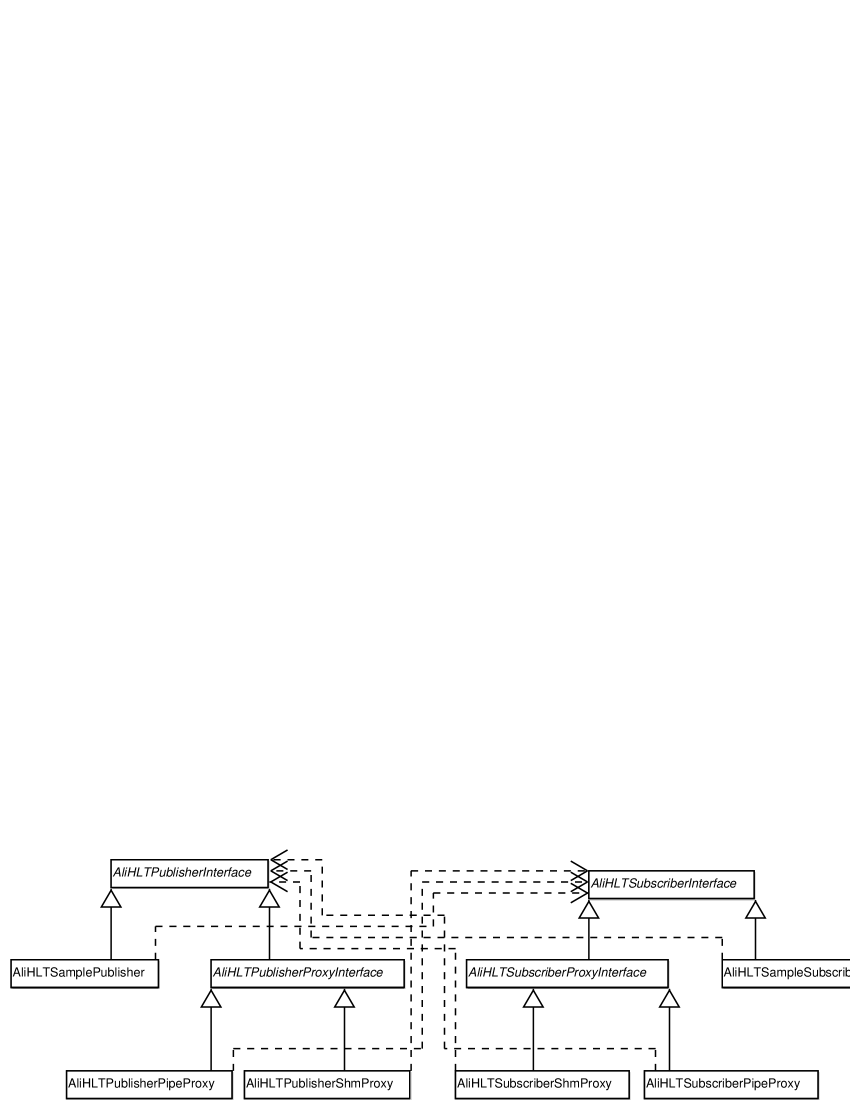
Two separate class trees, displayed in Fig. 6.1, make up the class hierarchy for the publisher and subscriber part of the framework respectively. At the root of each tree is an abstract base class that defines the calling interface of the corresponding part of the component interface. Each class in one of the two trees addresses its counterparts in the other tree through this defined interface.
The model behind the component interface is a data producing component containing a publisher object through which it makes its data available. A data consumer component contains a subscriber object which receives published data from a producer and performs the necessary processing on it. Communication between these two object types should be encapsulated so that they can communicate when they are situated in different processes and address spaces as well as when they are present in the same process, directly calling each others functions. For this reason the implementations of the two classes use the interface of their respective opposite tree and do not contain any built in communication primitives. Communication between objects in different processes is handled by proxy objects that implement the corresponding opposite interface and do not process the calls but only forward them to their own counterpart in the remote process who calls the target object’s corresponding function. These communication classes are called publisher and subscriber proxy classes respectively. The advantage of this approach is that publisher and subscriber object can be either situated in separate processes, calling functions of proxy objects for communication with their counterpart, or in the same process, directly calling each other’s functions.
An example of this principle is sketched in Fig. 6.2 which shows a producer process containing a publisher object and a subscriber proxy as well as a consumer process with a publisher proxy and a subscriber object. When new data is available the publisher calls the subscriber proxy’s new data function which collects the specified information and sends it to the publisher proxy in the consumer process. This proxy retrieves the received information and calls the subscriber object’s new data function with this data. As soon as the subscriber object in the consumer process has finished processing the data, it calls the publisher proxy’s data finished function. The publisher proxy again uses the specified data and sends it to its subscriber proxy counterpart in the producer process. Using this information the subscriber proxy calls the data finished function of the publisher object that can release the produced data and continue. Fig. 6.3 shows the same process as a UML sequence diagram.
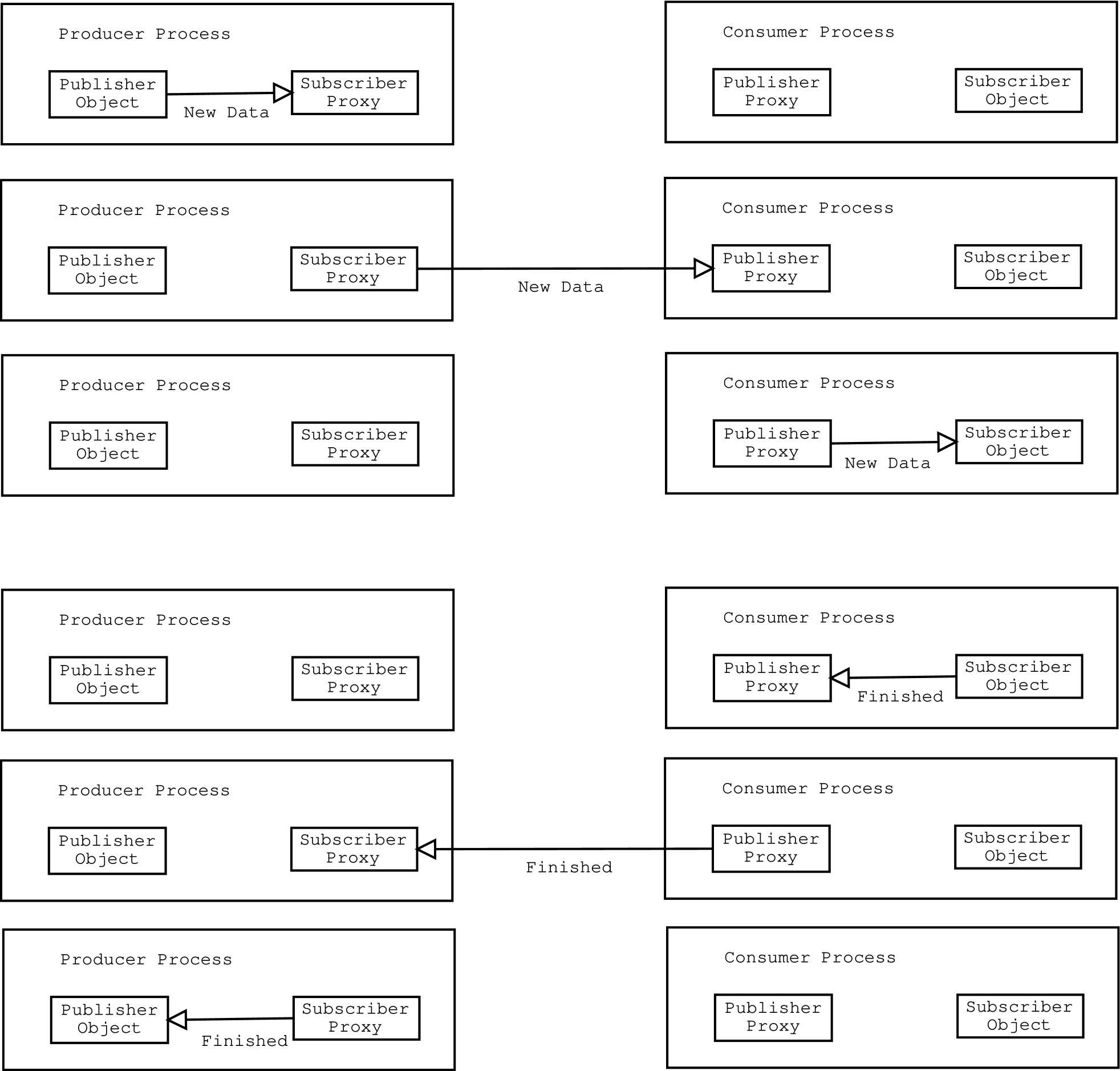
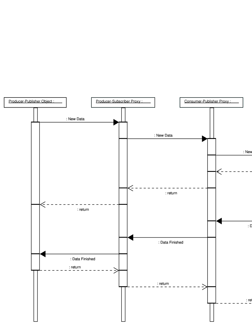
The primary purpose of the interface is to allow a data producer to announce newly available data, for example new ALICE events, to multiple subscribers. Placing the data in shared memory in the producer process implies that the management of the data’s buffers has to be handled by the producer process which needs to know where to place new data. In order for the producer to know when some specific data can be released again, it has to be informed by each of its subscribers when they have finished working on each received data block.
For efficiency reasons it should also be possible for consumers to collect finished events and inform their producer about multiple finished events in one call. During such an aggregation process by one or multiple consumers their producer process might run out of buffer space for new event data before the consumers have received and finished enough events to inform the producer about their released events. In such a case a producer has to be able to send a high watermark to its consumers when it threatens to run out of buffer space. For a non-blocking or transient type of consumer, a producer must also be able to forcibly cancel a consumer’s access to an event’s data buffers. This is necessary to free a buffer when the consumer uses and thus locks the buffer too long.
In some cases it might be desirable for a consumer to send some data about the processing of an event back to the producer along with the finished event information. An example for this in the ALICE HLT are the HLT trigger decisions for an event that have to be communicated back along the path that the event data has taken. To support this ability, the calls informing about finished events allow to attach arbitrary information to each event. This information is treated as opaque to the interface itself and is just transported from subscriber to publisher. For some consumers it might also be of interest to receive this kind of event finished information produced by other consumers attached to the same producer. Support for this is provided by allowing the subscriber to set a flag in their publisher to indicate interest in this information. Whenever new event finished information becomes available afterwards it will be forwarded to this consumer.
For consumers that want to reduce the amount of data or events they receive from their producer two approaches are possible that can also be used in combination. The simpler possibility is to set a modulo restriction based on the event sequence number so that only events with a sequence number evenly divisible by that specifier will be published to the consumer. The more complex but also more flexible approach allows to use tags called trigger words associated with each event. A consumer has the possibility to specify a set of trigger words, and only events that have a correct trigger word set will be announced to that consumer.
One final necessity for the interface is that each side has to be able to query whether its partner process is still alive. This is accomplished by using ping calls which must be answered within a predefined time by an acknowledge call. If this answer is missing, the partner can be presumed to be locked up or have terminated.
In the rest of this chapter first a number of basic data types used in the interface’s implementation are presented. In the following the definitions of the central interface classes as well as the proxy classes, used for communication between publisher and subscriber processes, are described. The final two parts respectively describe implementations of publisher and subscriber classes providing actual functionality.
6.2 Auxiliary Data Types
In the following section a number of datatypes will be described that have been defined for use in the publisher-subscriber interface. These types are used in the definitions of both publisher and subscriber class interfaces. The first subsection 6.2.1 lists simple datatypes with no or very little inner structure while the following subsection 6.2.2 contains the descriptions for more complex structured data types.
6.2.1 Flat Types
Integer Types
To ensure type compatibility in a system that can use multiple node architectures a number of unsigned integer types have been defined that always have the same size and thus value range on different systems. The definition is made from the basic datatypes defined for the C/C++ language using #ifdef preprocessor directives. Four different tpes are defined with 1, 2, 4, and 8 bytes (or 8, 16, 32, and 64 bits), named AliUInt8_t, AliUInt16_t, AliUInt32_t, and AliUInt64_t respectively. For the 64 bit type an exception has to be made as a type of that size is in general not supported by compilers on 32 bit platforms and so a GNU Compiler extension, the unsigned long long datatype, had to be used.
The Event ID
For identification purposes each event has to be tagged with a unique ID. The AliEventID_t datatype used for this task is simply defined to be identical to the previously declared 64 bit unsigned integer type AliUInt64_t. Depending on the application equal sized structures can be overlaid over this flat datatype. The most simple possible use would be to just encode a unique sequence number into this type. A more complex use could store a timestamp, as for example returned by gettimeofday, using the higher 32 bits for the second portion and the lower 32 bits for the microseconds.
The Node ID
Unique identification of the nodes in a cluster running a data flow chain is provided by the AliHLTNodeID_t datatype. As it is assumed that every node in such a cluster will be equipped with at least one TCP/IP network interface, the 32 bit IP address of that interface is used as the node’s ID. To store this address ID the AliHLTNodeID_t type has been defined to be the 32 bit unsigned integer AliUInt32_t type. In the case of multiple interfaces and IP addresses for one node the first address returned by the gethostbyname system call will be used.
6.2.2 Structure Types
The Data-Type Specifier
To allow the specification of the type of data stored in a memory block, the AliHLTEventDataType type was introduced. It is basically again the 64 bit large unsigned integer AliUInt64_t overlayed with an additional structure as an 8-character-array. This array overlay allows to print the datatype, for example for debugging purposes. The prerequisite to this is that the data type is specified in a format such that each of the 8 characters is actually printable. For the application in the ALICE High Level Trigger “ADCCOUNT”, “CLUSTERS”, or “TRACSEGS” are among the possible values.
The Data-Origin Specifier
In analogy to AliHLTEventDataType, the AliHLTEventDataOrigin type allows to specify the origin of the data stored in a memory block. It uses the same principle of overlaying an array of 4 characters over a 32 bit AliUInt32_t ID. For the ALICE HLT this can contain the detector where the data originated from. Possible values are “TPC “ or “DIMU” for the TPC and DiMuon arm respectively.
The Shared Memory Identifier Structure
This structure, named AliHLTShmID, holds the information required to access the shared memory areas where event data published by a data producer process is stored. It contains two fields, the first of which is an AliUInt32_t member that defines the type of the shared memory segment. Possible values currently define an invalid segment, a big physical area shared memory segment (bigphys), or a shared physical memory segment (physmem). In the second field the actual ID of the shared memory segment is contained in an overlayed AliUInt64_t/8-character-array organization as described above.
The Basic Structure Header
Every complex data structure that will be passed between processes will contain at its beginning an instance of this AliHLTBlockHeader header structure. To allow for an opaque transport of such structures, the header contains as its first element a 32 bit unsigned integer holding the length of the whole structure in bytes. The next two fields allow to specify the type of the structure as a type and subtype combination. Both use the unsigned integer/character array overlay principle of the two preceeding types, with a 32 bit/4 byte size for the type field and 24 bit/3 byte size for the subtype. The last field in the header structure is an 8 bit unsigned integer carrying a version number for each structure type which allows to add elements to a structure.
The Sub-Event Data Block Descriptor
Information describing a block of data stored in shared memory is contained in the AliHLTSubEventDataBlockDescriptor structure type. Since a block descriptor will not be exchanged between processes by itself but only as part of a AliHLTSubEventDataDescriptor structure described below, it does not contain an instance of the header structure discussed above. The first element of the structure is the ID of the shared memory segment holding the described data in the form of an AliHLTShmID field. Following this there are two 32 bit unsigned integer fields that contain the starting offset of the block relativ to the beginning of the shared memory segment and its size in bytes.
Behind these fields required to access the data, five more fields are defined which describe the data in the shared memory itself. The first of these is the ID of the node that produced the data, followed by two fields with the type of the data and its origin. Each of the three fields is of the corresponding type described above. Finally, two 32 bit unsigned integers are available, the first of which can contain a specification of the data under the control of each application while the second contains the byte order that the data has been stored in. Fig. 6.4 shows the definition of this type.
struct AliHLTSubEventDataBlockDescriptor
{
AliHLTShmID fShmID;
AliUInt32_t fBlockSize;
AliUInt32_t fBlockOffset;
AliHLTNodeID_t fProducerNode;
AliHLTEventDataType fDataType;
AliHLTEventDataOrigin fDataOrigin;
AliUInt32_t fDataSpecification;
AliUInt32_t fByteOrder;
};
If the datatype of a block has the value “COMPOSIT”, then the data block described contains another AliHLTSubEventDataDescriptor structure described below, allowing hierarchical event descriptions.
The Sub-Event Data Descriptor
To describe the information for a whole subevent the AliHLTSubEventDataDescriptor can be used. This structure’s first element is a header of the AliHLTBlockHeader type followed by an AliEventID_t field containing the ID of the event concerned. The next two elements are 32 bit unsigned integers holding event time information, the seconds and microseconds of the timestamp of the event’s creation. After these elements another 32 bit unsigned integer is placed that contains a timestamp specifying the maximum allowed event age in the system. This timestap is specified in seconds as returned by the Unix time function. Using it information can be broadcast through a system to purge events from the system that have not been freed properly, preventing the slowing down or filling up of the system.
The sixth field of the structure contains the datatype of the whole event. If all the datablocks of the event are of the same type, then this field can contain this datatype specifier. Otherwise this field contains the specifier “COMPOSIT” to indicate a composite event. Behind this field there is another AliUInt32_t element holding the number of data blocks contained in this descriptor followed by the corresponding number of AliHLTSubEventDataBlockDescriptor structures containing the information for each of the data blocks. Fig. 6.5 shows this type’s definition.
struct AliHLTSubEventDataDescriptor
{
AliHLTBlockHeader fHeader;
AliEventID_t fEventID;
AliUInt32_t fEventBirth_s;
AliUInt32_t fEventBirth_us;
AliUInt32_t fOldestEventBirth_s;
AliHLTEventDataType fDataType;
AliUInt32_t fDataBlockCount;
AliHLTSubEventDataBlockDescriptor fDataBlocks[0];
};
Hierarchical event descriptions are supported by allowing data blocks to contain locations of further AliHLTSubEventDataDescriptor structures, placed in shared memory as described in the previous section.
The Event Trigger Type
In the AliHLTEventTriggerStruct data is contained that characterizes a particular event and allows a subscriber to select only a particular subset of events for processing. For applications in high-energy or heavy-ion physics this could be trigger information received from preceeding trigger levels specifying a type of event. Since the organization of this type of data cannot be known in advance by the framework, this type has no complex inner structure. It contains only the header field as well as an AliUInt32_t holding the number of 32 bit data words in the structure and another AliUInt32_t marking the beginning of the data word array. For determining matches between structures a comparison function type is defined. A comparison function which performs a bytewise comparison of two structures is supplied in the framework.
The Event Done Data Type
The structures of the AliHLTEventDoneData type contain information transferred back from a subscriber to a publisher about events whose processing has been finished. This additional information in these structures is opaque to the framework, which only transports the data for interpretation by the higher layers of the system’s components. Therefore, application specific data is implemented similarly to the event trigger type described previously, as one 32 bit unsigned integer holding the number of data words in the structure followed by the array of 32 bit unsigned data words itself. Preceeding these fields are the usual header structure and a field with the ID of the event concerned. In the following text the expression “non-trivial event done data” will be used to describe an event done data structure that contains at least one 32 bit data word.
6.3 The Interface Definition Classes
6.3.1 The Publisher Interface
Fig. 6.6 shows the interface for publisher classes, AliHLTPublisherInterface, as a UML class diagram. This interface defines abstract methods for each of the tasks described in section 6.1. In the AliHLTPublisherInterface class one data member and one non-abstract member function are contained. The data member holds the name under which the publisher referred to by an object is known. It is returned by the GetName member function.
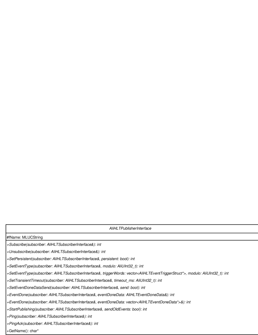
The first two of the methods defining the publisher interface, Subscribe and Unsubscribe, handle subscribing and unsubscribing to a publisher. Both methods accept as only parameter a reference to the subscriber to be subscribed to. Once a subscriber object is subscribed to a publisher, its type can be set with the SetPersistent method. It requires a reference to the subscriber concerned as its first parameter together with a boolean flag specifying whether the subscriber should be treated as persistent or transient. Initially after subscription, all subscribers are marked as persistent requiring the method to be called for transient subscribers only.
Using the two following SetEventType functions, it is possible to scale down the number of events received by a subscriber from its publisher. In the first of the functions the event sequence modulo specifier is set that scales down the event rate to the given ratio. Only events whose sequence number is evenly divisible by the specified modulo number will be announced to this subscriber. The second variant of the functions accepts a vector of trigger word structures, described in section 6.2.2, together with a modulo specifier identical to the one passed in the simpler function’s version. Specified trigger word structures are stored associated with the subscriber, and each new event is checked for a match with one of them.
A method of interest to transient subscribers only is SetTransientTimeout. It allows to set the minimum timeout before an event used by a transient subscriber can be cancelled. A publisher will cancel a transient subscriber’s event only when all persistent subscriber have released it and at least the amount of time specified in this call has passed. To prevent transient subscribers from setting arbitrarily large intervals it is suggested that publisher implementations have a separate allowed maximum for this timeout. Transient subscribers should thus be prepared for shorter timeouts than specified. The last subscriber configuration method is the SetEventDoneDataSend method, that also uses a boolean flag as its parameter. This flag specifies whether the subscriber concerned is interested in receiving the data sent along with finished events from other subscribers. Since this information might be needed by the subscriber to properly process the event, this information is forwarded immediately after another subscriber has released a specific event in the publisher.
To inform a publisher that processing of an event has finished, a subscriber calls one of the two EventDone methods in the publisher interface that differ only with respect to the arguments taken. In the first call one AliHLTEventDoneData structure argument, described in 6.2.2, is accepted to release only one event while the second version allows to release multiple events in one call by accepting a vector of these structures. As described previously, each of the structure arguments contains the identifier of the event to be released.
By calling the StartPublishing method, a subscriber activates publishing of new events for itself. After calling this method a subscriber will receive all new events as they become available in the publisher. This call will not return immediately but instead will enter a loop until Unsubscribe has been called. The final two methods are used by a subscriber to test a publisher’s availability (Ping) or to reply to a publisher to acknowledge the subscriber’s own availability (PingAck). An optional boolean flag, which can be given as the second parameter, allows to specify that all events currently contained in the publisher, already announced to other subscribers, should be announced to the subscriber concerned. If this flag is not set, only events which arrive in the publisher after the StartPublishing call will be announced.
6.3.2 The Subscriber Interface
Fig. 6.7 shows the interface for subscriber classes AliHLTSubscriberInterface as a UML class diagram. This interface defines abstract methods for each of the subscriber tasks described in section 6.1. Similar to the publisher interface class AliHLTSubscriberInterface also contains the subscriber’s name as the only data member and the non-abstract member function GetName to return that name. In analogy to the publisher interface all defined abstract subscriber interface functions require a reference to the publisher object calling the corresponding subscriber function as their first argument.
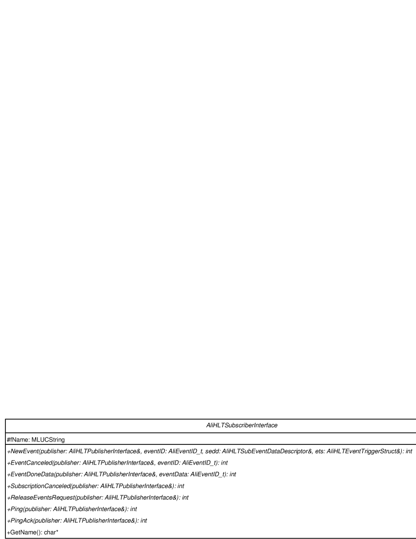
NewEvent, the first of the abstract member functions defined for the subscriber interface, will be called when the publisher to which the respective subscriber is attached announces new data. It is therefore the most important subscriber member function. In addition to the calling publisher’s reference it accepts three more arguments. The first of these is an AliEventID_t containing the ID of the event being announced. Following is an AliHLTSubEventDataDescriptor holding the information about the actual data blocks contained in the event, mostly located in shared memory. The final argument is an event trigger structure of the AliHLTEventTriggerStruct type, containing information that more closely characterizes the event concerned. Event trigger data is passed to the subscriber so that it can determine the processing of the event based on this trigger information.
The second abstract subscriber interface function is EventCanceled. It is called for transient subscribers whenever the publisher to which they are attached cancels an event before the subscriber itself has finished working on it. After this function has been called a subscriber should not rely on any data located in shared memory to still be valid. Processing on this event should be stopped as soon as possible after this function has been called. Parameters to this function are the calling publisher’s reference and the ID of the event being cancelled.
Next is another notification function, that can be called while any subscriber has not yet finished processing an event. EventDoneData is called when the publisher receives event done information from another subscriber and this subscriber has requested to receive this kind of data using the publisher’s SetEventDoneDataSend function. The function will be called with the exact AliHLTEventDoneData structure that the publisher received from the other subscriber, provided that the structure is non-trivial, containing at least one data word.
When the publisher cancels a subscription the SubscriptionCanceled function of the subscriber concerned is called. Such a cancellation might happen because the subscriber has called the publisher’s Unsubscribe function or because the producer process is ending. Each subscriber’s ReleaseEventsRequest function is called when the publisher threatens to run out of buffer space to signal that the subscribers should release events as soon as possible. The final abstract member functions defined for the subscriber interface are the Ping and PingAck functions that have the same meaning as the respective functions in the publisher interface described in section 6.3.1.
6.4 The Proxy Classes
Beyond the functions defined already in the publisher and subscriber interface definition classes, two derived classes exist defining additional interface functions for the two types of proxy classes. These two interface classes are shown in Fig. 6.8 with their respective, additionally defined functions.
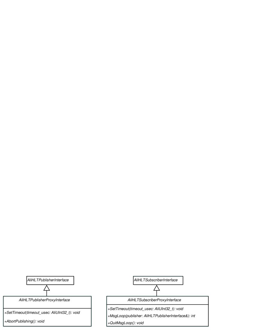
Both classes define a SetTimeout function allowing to specify a communication timeout used by proxy implementations in a program. Since only the proxy classes are intended for communication between processes, but not publisher or subscriber classes in general, it is reasonable to place this function in these classes. The AliHLTPublisherProxyInterface class defines one additional abstract function, AbortPublishing. Its purpose is to terminate the publishing loop started by the proxy classes when their StartPublishing function is called as described below. Usually this function ends when a SubscriptionCanceled message is received from the publisher. If, however, the publisher process has died or the connection between publisher and subscriber processes is interrupted or broken, the publisher proxy cannot determine when to leave the message loop.
Two additional functions are defined in the AliHLTSubscriberProxyInterface class, MsgLoop and QuitMsgLoop. The MsgLoop function is intended to contain the implementation of the proxy’s loop for receiving and handling messages from the opposite publisher proxy in derived classes. It should be called in a separate thread from the publisher object to which the proxy is attached. When the loop has to be terminated because the subscription has been cancelled, the publisher calls the third defined function, QuitMsgLoop, whose purpose is to end the message loop.
In the following section the proxy classes present in the current framework are described. They can be divided into two types categorized by the type of communication between publisher and subscriber proxies: pipe proxies and shared memory proxies. Communication for the two pipe proxy classes is done via named pipe [124] system resources while the shared memory proxies communicate via System V shared memory [120], [121], [122], [124]. In addition to these four proxy classes the final part of this section covers the subscription loop, the mechanism for subscribers to register with publisher objects in other processes.
6.4.1 The Pipe Proxy Classes
The Pipe Communication Class
Named pipes used for communication between the pipe proxy classes are encapsulated by the AliHLTPipeCom class. This class supports two pipes simultaneously, one for reading and one for writing, as the pipe communication between the proxies is executed via two named pipes. One of these is used for communication from publisher to subscriber and the other from subscriber to publisher. Two pipes are used to avoid lockup situations. The naming of the pipes is based on a scheme that places all pipes in the /tmp directory and assigns a base name identical to the subscriber’s ID to them. Each pipe has an additional suffix, either PublToSubs or SubsToPubl depending on the flow of communication. The full file names for a subscriber whose ID is TestSubscriber then are /tmp/TestSubscriberPublToSubs and /tmp/TestSubscriberSubsToPubl. The pipe class offers an interface for reading and writing similar to the system read/write function calls. This interface allows direct specification of the number of bytes to read or write together with a memory block where the write data was stored, respectively where read data should be stored. Functions of this interface are shown in Fig. 6.9.


In addition, a second interface is supported that directly allows to read and write structures described by an element of the AliHLTBlockHeader type, detailed above in section 6.2.2. This interface is shown in Fig. 6.10. For writing, this version of the Write function requires a pointer to such a block header structure as its primary argument. It will write as many bytes from the memory pointed to as specified in the header’s length field. In the Read function the header structure is read first and then the required amount of bytes is allocated as specified in the header’s length field. The header already read is copied to the beginning of this memory block and the rest of the data is read and placed directly into that memory. In the function’s pointer reference argument the pointer to the allocated memory is then returned to the calling code that later has to free the allocated memory again through a call to delete [].
To avoid blocking, e.g in case a process attempts to write to a pipe that has been filled because the reader process has died or locked up, all read and write function calls accept an additional boolean argument specifying whether the call is to be blocking or non-blocking. For non-blocking calls a member variable in the pipe object is used that specifies the timeout to use when a call would block. This timeout can be specified on a microsecond granularity.
In order to reduce the number of system read calls in a more efficient reading mechanism, the pipe communication class implements a caching strategy, similar to what is implemented in the BCLIntTCPComHelper class described in section 5.4.2. Each object contains a buffer of 4 kB size, the maximum amount of data that can be read from or written to a pipe in one system call. If this buffer is empty upon a read call, the object tries to read the full amount of 4 kB into this buffer at once. Since the pipes are opened in non-blocking mode the read attempt will read as much data as is available up to the specified amount. Data that has been requested by the calling code will be provided from this cache until it is exhausted, saving a number of read calls.
The Publisher Pipe Proxy Class
Handling the publisher part of the communication based on named pipes is the task of the AliHLTPublisherPipeProxy class, implementing the abstract functions defined in the publisher interface. Two named pipes, provided by an instance of the AliHLTPipeCom class described above, are used for the two communication directions. Additionally, the proxy uses a third named pipe, encapsulated in another pipe object, for connection to a publisher’s subscription loop, as described below in section 6.4.3. This pipe object uses just one of the two possible pipes as no reading will be done from it, and only the subscription request will be written. Fig. 6.11 shows the UML relationship of the proxy class and the pipe communication class.
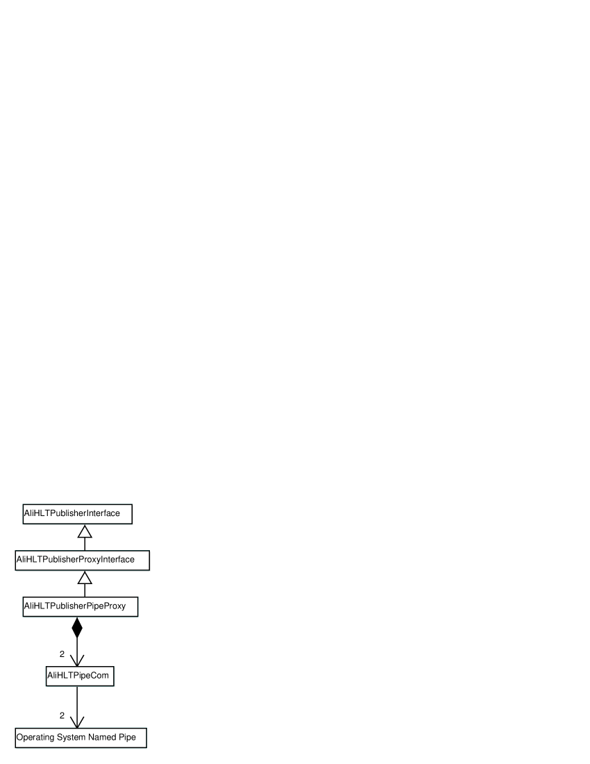
In the Subscribe function the publisher pipe proxy first tries to open the subscription request pipe to the producer process’s subscription loop. Then the two pipes used for the actual communication between the publisher and subscriber processes are created. It is mandatory that these pipes are created by the publisher proxy in the subscriber process and that they are already present when the subscription request is written into the request pipe. The subscription message sent to the publisher contains the subscriber’s name field as its identifier, preceeded by the string “pipe:” to specify that pipe proxies are used. After its construction this message is written into the subscription pipe and the Subscribe function ends.
To unsubscribe none of these steps have to be executed by the Unsubscribe function. Instead it starts by creating the unsubscription message. This message also contains the subscriber’s name as the identifier. Again the function ends immediately after writing the message into the pipe for subscriber to publisher communication. This communication can also be seen as communication between a publisher proxy in the subscriber process and a subscriber proxy in the publisher process.
Both messages created in the functions described contain the block header structure as their first element. They can be written into their respective pipes via the block header write functions. For the rest of the functions the messages follow the same principle. Any additional parameters needed by the messages are encapsulated into data structures that contain this header structure as well and can also be written using the header write functions.
For efficiency reasons, calls which accept parameters and that thus have to send multiple structures do not actually send each structure with a separate write call. Instead a coalescing step is taken where a block of memory is allocated with a size large enough for all data to be sent. The message, all parameters, and any additional data are then copied into that block, and the block is passed to the pipe object for writing using a single call to the Write function. When the allocation of the buffer block fails, seperate calls to the block header Write function are used.
At the end of the StartPublishing function, after the message and parameters have been written, the function does not return but instead enters the message loop function. In this loop the publisher proxy waits for messages that arrive on the publisher-to-subscriber pipe. Received messages are checked for the correct header identification and are then handled according to their respective type. For most of the messages, reading of the necessary parameter structures and their decoding into normal C++ parameters is done in separate functions. In these functions the parameter structures are also checked for the correct header identification. Once the C++ parameters have been obtained the corresponding function in the attached subscriber object is called with these parameters. When the message corresponding to the SubscriptionCanceled method is received, the message loop is ended normally.
To ensure the correct transport of the data through the named pipes, the publisher proxy class has the ability of performing a 32 bit Cyclic Redundancy Checksum (CRC) [128] over the data for each message including its parameters. This checksum is sent after the actual data. In the subscriber proxy’s receiving message loop the same checksum is calculated using the received data. The subscriber proxy’s checksum is then compared with the value calculated and sent by the publisher proxy. If the comparison indicates that an error occured, this is reported, and the received data is discarded without further action. The publisher proxy message loop and the subscriber proxy functions implement the identical error checking mechanism. This capability can be activated using #define statements at compile time of the classes.
The Subscriber Pipe Proxy Class
In the producer process it is the AliHLTSubscriberPipeProxy’s task to handle the subscriber part of the named pipe communication. For this purpose it implements all abstract functions defined in the subscriber proxy interface. This class uses only one pipe communication object to handle the same two publisher-subscriber pipes. The meaning of the pipes with regard to reading and writing is of course reversed with respect to the publisher proxy class. A subscriber proxy object is created in the producer process only when a subscription has taken place, and the pipes are created at the beginning of the publisher proxy’s Subscribe function. Therefore the pipes will exist already upon creation of an object of this class. In the class’s constructor they thus only have to be opened. Fig. 6.12 shows a UML diagram of the relationship between the proxy and pipe communication classes.
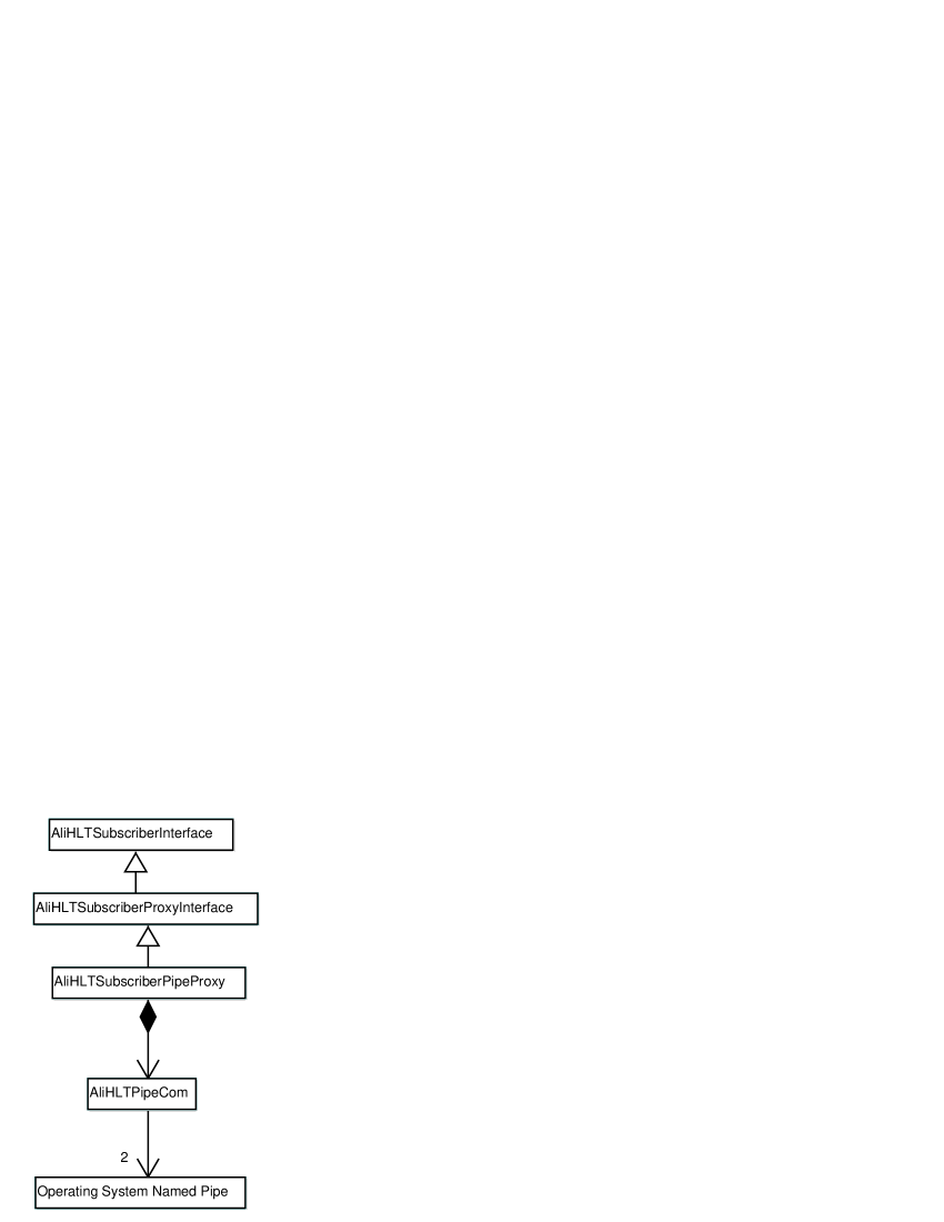
As for AliHLTPublisherPipeProxy, the implemented interface functions mainly create a message object, identical to the publisher proxy’s message object, and several parameter objects as required to hold the necessary arguments. These data structures are then coalesced and sent utilizing the same mechanisms as used in AliHLTPublisherPipeProxy. Only if the coalesced sending call fails, the structures are sent with separate Write calls for each of them. The subscriber proxy’s functions and its message loop implement the same optional CRC error checks as the publisher proxy, as has been described in the previous section.
Unlike the publisher proxy class, no call to one of the interface functions causes a subscriber proxy object to enter the message loop function defined for subscriber proxy objects. Instead the message loop has to be called explicitly by a publisher object after a proxy object has been subscribed to it, for concurrency preferably in a separate thread. In analogy to the publisher proxy class the message loop calls functions to handle the more complex messages with multiple arguments for parameter extraction. Using the extracted parameters, the proxy calls the appropriate interface functions in the publisher object to which it is attached. A further difference to the publisher proxy class is that the message loop does not automatically end when a specific message is sent or received. As is the case for starting the loop, it has to be terminated explicitly by a call to the QuitMsgLoop function from the parent publisher object.
6.4.2 The Shared Memory Proxy Classes
The Shared Memory Communication Classes
In analogy to the pipe communication class for the pipe proxies, the two shared memory proxy classes also rely on a common base class, AliHLTShmCom, to handle the interaction with the System V shared memory functions. In addition, the class also handles the buffer management for the shared memory blocks used for communication between the proxies.
Since System V shared memory segments cannot be identified by names but only by integer IDs, such an ID has to be passed to the communication object together with the segment’s size. These two arguments are passed to the object’s constructor where the shared memory segment will be created or opened. To support the case where a communication partner connects to a segment already created by its partner, the class’s constructor accepts a flag argument. This flag allows to specify whether the object should create the segment specified or whether it should just try to connect to an existing segment.
One problem encountered in communication via shared memory is that it does not support suspending a process while waiting for data, notifying and waking it up when data has become available. Similarly, it is not possible to wait when no space is available for writing, to be notified after enough space for the attempted write operation has again become available. If one were to use continuous polling of the parameters that indicate available data, this would result in a high CPU load on the system. As a compromise the approach chosen for this class uses a number of read or write attempts followed by usleep calls. The usleep calls use the minimum granularity available to processes on a Linux system of 10 ms. To reduce the impact of this rather high sleep time, the number of poll retries executed before sleeping can be configured for each object during runtime.

Similar to the pipe communication class the shared memory communication class also supports multiple kinds of read and write calls, although in this case they do not just differ in ease of use but also in the degree of efficiency supported. The first function set for reading and writing in Fig.6.13 works identical to the basic functions provided in the pipe communication class. Both functions accept a size specifier for the amount of data to read or write and a pointer to the data buffer. Their final parameter is a flag, specifying whether the call should block indefinitely or use a specified timeout. Using this interface the data is copied by the CPU from the source memory to the destination by memcpy calls.

The second call interface, shown in Fig. 6.14, only provides two functions to allow reading, while no support for data writing is present. These functions contain support for reading data structures described by a block header structure at their beginning, analogous to the second interface type of the pipe communication class. Unlike the two functions from the first set, this interface does not always perform copy operations for the data. Instead the first of the two functions can return a direct pointer to the data structure located in the shared memory segment, avoiding the copy steps. To prevent overwriting of data while it is still in use, the occupied memory is not directly marked as available again. This is performed by the second function of this set, which can be called when the read data can be released. Copy steps are only necessary if the read data, described by the header structure, is wrapped around in the buffer. In such a case the first part lies at the buffer’s end and the second at its beginning. This situation is handled by allocating a further memory block of the required size and copying the data from the shared memory buffer into that memory by two memcpy calls. The allocated memory is returned as the pointer to the block header structure. When the free function is called in this case it does not only release the memory in the buffer but also frees the specifically allocated memory again. In the first of the two functions, Read, five arguments are accepted. Only the first and last of these arguments are relevant to the user. The first is a reference in which the pointer to the structure will be returned and the last is an optional flag that indicates whether or not the function should block while waiting for data. Two pointers and a size specifier make up the remaining three arguments in which information is returned from the function that the second function, FreeRead, uses to determine whether the memory with the data has been allocated or is in the shared memory. Except for the block argument, which does not apply to the free operation, the remaining four parameters supported by the Read function have to be passed in the call to the FreeRead function to provide it with the required information to release the block or blocks.

The third interface, shown in Fig. 6.15, also allows a more efficient approach to communication by using a set of two functions for writing and three for reading. For writing only the size of the data to be written is passed to the first of the two functions, CanWrite, together with a flag specifying blocking or non-blocking mode. Three parameters are returned by the function, two pointers and another size specifier. When the memory block for writing the specified amount of data is present as one block in the shared memory buffer, then the second pointer and the returned size specifer are both zero. In the first pointer parameter a pointer to the target block in shared memory is returned. In contrast, when the block for writing wraps, then the first pointer points to the part of the block located at the buffer’s end and the second pointer to the one at the buffer’s beginning. The returned size specifier contains the size of the block’s first part located at the buffer’s end. Using the two pointer arguments, the data can then be written into the shared memory buffer. To avoid copying, the data can even be directly created in the shared memory, taking into account the two parts of the block. Once the data is present in the buffer, the second function HaveWritten can be used to commit it and make it available for reading. HaveWritten requires the first four of CanWrite’s parameters, the fifth blocking parameter is not applicable. Using these parameters it determines whether the block is in one piece or wrapped around and then accordingly sets the amount of data written in the object’s internal structures.
Of the three functions available for the read part of this interface, two CanRead functions are used to determine whether data is available for reading. These functions only partly differ in their arguments, having five of them in common: a size parameter specifying how many bytes to read, two pointer arguments, a second size specifier, and a blocking/non-blocking flag. In combination the two pointer arguments and the additional size specifier basically have the same function as in the CanWrite function, specifying the memory where the data to be read is located either as one block or as two wrapped around parts. The difference between the two functions is an initial flag argument, available in one of the functions. The flag specifies whether the read indices should be updated and mark the data whose pointers are returned as read, or whether the function should just peek for available data and not modify any indices. In the function without this additional flag argument the first CanRead function is called with all its specified parameters and the peek flag set to false. This function will thus mark the data as read so that the next CanRead call will return pointers to the next available data block. Once the data has been accessed and can be released, the third function, FreeRead, is available to release the data and make the memory blocks usable for writing new data. This function requires the two size and pointer arguments of the CanRead functions and updates the indices of the object to mark the block concerned as free.
The Publisher Shared Memory Proxy Class
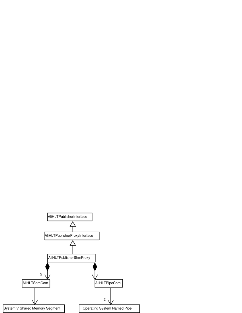
Similar to the AliHLTPublisherPipeProxy, the task of the AliHLTPublisherShmProxy class is to handle the publisher side of the shared memory communication in the data consumer processes. It uses two shared memory communication objects for the two communication directions from publisher proxy to subscriber proxy and vice-versa. Each of these requires its own shared memory key, although both use the same size. The communication objects and their memory segments are created by the class’s constructor. In addition to the two shared memory segments, one pipe communication object is used to execute the subscription through the publisher’s subscription loop described below in section 6.4.3. AliHLTPublisherShmProxy’s hierarchy and its relation to the two communication classes is shown in Fig. 6.16.
The subscription pipe is opened in the class’s Subscribe function using the publisher’s name specified in the object’s constructor, in order to build the pipe name as described for the publisher pipe proxy in section 6.4.1. Since the shared memory segments have already been created the subscription request message can be sent directly. This message includes the subscriber’s name preceeded by ’shm:’ to indicate that a shared memory proxy is used. Following the name the message contains the rest of the information needed by the publisher to establish a communication: the two shared memory keys and the segments’ common size.
In the implementations of the functions defined in the subscriber interface, the approach used is basically always identical. The function determines the total amount of data that it has to write for the message and its required parameters. This size is then passed to the call of the CanWrite function of the publisher-proxy to subscriber-proxy shared memory object to obtain the shared memory block for writing the message. If this block in the shared memory segment consists of only one part and is not wrapped around, then the message and its parameters are created directly in the memory block just allocated. Additional data can be copied from function parameters as necessary. If the data is not in one block but wrapped around, an additional memory block is allocated and the message and parameter creation functions are called using this local memory block. Once all the required message data is present in this block it is copied into the two parts of the shared memory block through two memcpy calls. After these steps the HaveWritten function is called to commit the data and update the write indices in the communication object appropriately. Once this is done all functions except for StartPublishing end, indicating successful completion to the caller.
The StartPublishing function does not terminate once the message has been written into the communication object, but calls the class’s message loop to process messages received from the producer processes’ subscriber proxy, similar to the publisher pipe proxy. In the loop the messages received from the subscriber proxy are read using the block header read function of the subscriber-proxy to publisher-proxy communication object described earlier. For the three messages NewEvent, EventCanceled, and EventDoneData that require multiple parameters, handler functions are called to read the necessary parameter data from the communication object. The parameters are subsequently decoded and the appropriate function in the attached subscriber object is called with them. For the other, simpler, messages the subscriber functions can be called directly without the need for further parameters. After calling the appropriate subscriber’s functions the data in the shared memory is released again using the appropriate FreeRead calls for the message and its parameters.
The Subscriber Shared Memory Proxy Class
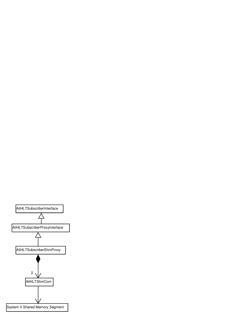
The subscriber shared memory proxy class AliHLTSubscriberShmProxy performs the subscriber proxy functions in the producer process, analogous the subscriber pipe proxy class described in section 6.4.1. For this purpose it implements the functions defined in the subscriber interface in a similar manner as in the shared memory publisher proxy class’s functions described in the previous section. Each function determines the size of the message to send to the publisher proxy together with necessary parameters and other data. Message data is created either directly in the shared memory buffer used for the subscriber-proxy to publisher-proxy communication, or it is created in an intermediate memory block and then copied into the shared memory segment.
As for the pipe subscriber proxy, no interface function called will cause a message loop to be entered. Instead the publisher to which this subscriber is attached to has to call the MsgLoop function, defined in the AliHLTSubscriberProxyInterface class, to run in a separate thread. Once the subscription has been cancelled the publisher has to call QuitMsgLoop to exit the message loop and terminate the thread.
6.4.3 The Subscription Loop Function
Related to the proxy classes is the subscription loop function PublisherPipeSubscriptionInputLoop which should be called by any producer process in a separate thread to wait for incoming subscription requests. Its only parameter is a reference to the publisher object whose subscription requests it should handle. From the object it obtains the publisher’s name used to create the full name of the subscription pipe so that it is located in the /tmp directory and consists of the name of the publisher with the appended SubsService identifier.
A pipe communication object as described in 6.4.1 is used to create and open a pipe with the constructed name. In the loop a blocking read is entered to wait for incoming messages with subscription requests. As each subscription request is contained in a single message described by a block header structure, a single Read call is sufficient to retrieve the data needed for a subscription. When a subscription request has been received, the function strips the type specifier, either pipe or shared memory, from the subscriber’s name to determine which type of proxy to create.
For a pipe proxy the only information needed is the name so that an AliHLTSubscriberPipeProxy object can be created directly. In the case of a shared memory proxy the function additionally has to extract the size of the two shared memory segments as well as the two keys for them from the message. Using these three parameters and the subscriber’s name an AliHLTSubscriberShmProxy object is created.
After the correct subscriber proxy object has been created the function calls its publisher object’s Subscribe function with the created proxy as its argument, subscribing the proxy and its associated subscriber object in the consumer process. Following this, the function releases the message that has been allocated in the pipe communication object and reenters the read call waiting for the next request.
When the subscription loop has to exit because the producer process ends, a global flag variable is set to be evaluated in the function’s loop. Subsequently, a quit message is sent to the loop’s named pipe. Upon reading that message and detecting the global quit flag set, the function leaves the loop and terminates.
6.5 The Publisher Implementation Classes
Only one publisher implementation class directly derived from the publisher interface definition AliHLTPublisherInterface exists, implementing the basic publisher functionality of managing a number of subscribers and events. Other publisher classes are in turn derived from this base class to extend its functionality. The most important of these classes, shown in Fig. 6.18, are described in the following section.
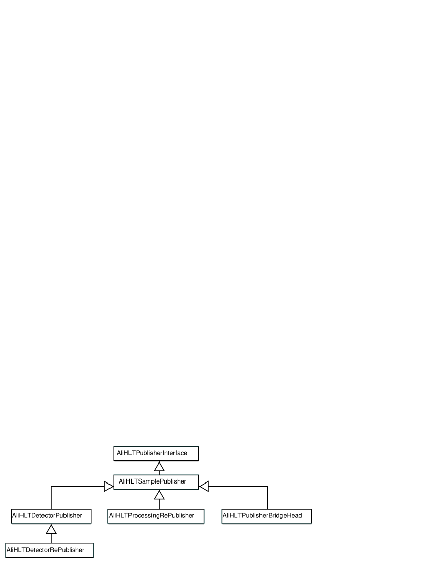
6.5.1 The Sample Publisher Class
AliHLTSamplePublisher is the base class for all other publisher implementation classes. It is the only class that implements the basic functionality of managing multiple subscribers, announcing events to them, and freeing the events again once all subscribers have released them. All other publisher classes inherit this functionality from AliHLTSamplePublisher. In addition to implementing the required abstract methods defined in the publisher interface it provides a set of other functions that serve as the external API of this class. It also supports a number of callback functions that allow for further customization of a derived publisher, e.g. by implementing an action when an event has been released. These callback functions are not defined as abstract methods so that not every derived class has to implement all of them but instead are present as empty virtual method bodies. The provided external API allows other programs or classes to use the features present in the sample publisher class, e.g. subscriber and event handling, management, and accounting.
Internal Architecture
Internally the AliHLTSamplePublisher class makes use of a number of different threads and two main lists that store the data for each subscriber and each event respectively. An entry in the subscriber list contains a pointer to the subscriber object or proxy, in the form of a pointer to a subscriber interface, together with pointers to two thread objects. These two threads are used for communication with the subscriber object. The first is used for the subscriber proxy’s message loop from which the publisher interface functions are called and the second for calling the subscriber object’s interface functions. This second thread object also implements the subscriber interface and can thus be accessed by the publisher class similar to a subscriber. Calls to the subscriber interface functions place the required data in a memory FIFO of the thread class. The thread itself runs a loop which waits for data from its FIFO object and calls the interface functions in the subscriber object, decoupling the publisher’s main functions from the timing behaviour of the subscriber object’s functions. This is of particular importance when the subscriber object actually is a proxy object that communicates with other processes and could block waiting for them.
A subscriber data structure furthermore contains a number of fields relevant to the subscriber’s status corresponding to the parameters that can be set using the respective publisher interface functions. Three flags define whether a subscriber is persistent or transient, whether it is active and receives events, and whether a subscriber receives event done data received from the publisher’s other subscribers. Additionally, three fields related to the data that can be set using the publisher’s SetEventType functions are present. Of these three elements the first is a list holding the event trigger type structures that can be specified. The other two are the event modulo number used to restrict the rate of events and the number of events that have been announced while the specific subscriber has been active. These two numbers are used to determine whether a specific event is announced to a subscriber with a set event modulo number. The final element in the subscriber structures is the number of ping calls that have been made to this subscriber. This number is increased when a Ping call is made to the subscriber object and decreased when a PingAck call is received from it. When the number reaches a configurable maximum the subscriber is presumed to be unable to process any calls and is removed in the publisher.
In each element of the event list a number of fields are stored as well. The first of these is the ID of the event whose data is stored in that particular element. This is followed by two reference counters, one for the total number of subscribers and one for the number of transient subscribers to which this event has been announced. Two more fields contain data regarding event timeouts, the maximum timeout used for that event and the ID of the currently active timeout for that event. Two sublists hold a list of subscribers which have not released the event that has been announced to them and a list of all event done data structures that have been received for that event. This last list is used for one of the callback functions presented below.
The event list itself is organized in a manner similar to the principle of the MLUCVector class described in section 4.2.2: a fixed size array used as a ring buffer. This approach is applied since events are typically processed in an approximate first-in-first-out manner. As the releasing of events is not guaranteed to be sequential, each entry in the list contains a used flag that specifies whether the data contained in the element is valid. Free slots for new events are always searched from the end of the used space while the search for events to be freed is started at its beginning. If no size for the array is specified in the class’s constructor, a normal dynamic array class, the vector class from the STL library, is used instead of the ring buffer.
Beyond the two communication threads for each subscriber, each sample publisher object uses four more threads in addition to a program’s main thread. The first of these is used to handle expired timeouts for each event. It runs in a loop waiting for signals from the timer object for expired timeouts. Any transient subscriber still locking an event with an expired timeout is forced to release the event. A loop waiting for timer signals is used in the second thread as well, but these timeouts signal expirations of wait times for ping messages. After a certain number of ping acknowledge replies have not been received, the subscriber concerned will be removed from the publisher’s list. Cleanup of subscribers in the process of being removed from a pulisher’s list is the task of the third publisher thread. Subscriber data structures are passed to this thread using a signal object. When the thread detects that a subscriber is not used anymore, it will free any data structures that have been allocated for this subscriber. It is necessary to use this approach to prevent a thread from releasing a subscriber when another thread still accesses that subscriber’s data structures. The final of these four threads runs the timer used for every timeout in the publisher, including event and ping timeouts.
External Sample Publisher Interface

Beyond the standard publisher interface for use by subscriber objects the sample publisher class provides a second function interface, shown in Fig. 6.19. This API consists of seven additional functions to be called from external functions, some of which correspond loosely to functions defined in either the publisher or subscriber interface. AnnounceEvent, the first of these seven functions, accepts the same three arguments as the subscriber’s NewEvent function: an event ID, a sub-event descriptor for the event’s data, and its event trigger type structure. The event described by these three parameters will be announced to subscribers currently attached to this publisher object, depending on the trigger types and modulo counters set for each subscriber.
To forcibly remove an event from a publisher’s internal list the publisher’s AbortEvent function can be called. The ID of the event to be removed is the function’s first parameter. An optional second parameter is a flag specifying whether an EventCanceled call is made to all subscribers that still use the event. By default this flag is true so that the EventCanceled calls are made. When a producer program starts to run out of buffer space for events, the RequestEventRelease function can be called to make ReleaseEventsRequest calls to all attached subscribers informing them of the imminent buffer shortage. To terminate all subscriptions or call the ping function for all attached subscribers respectively the CancelAllSubscriptions and PingActive functions are available, both without any parameters as for ReleaseEventsRequest.
In the case that releasing events in a publisher object has to be inhibited for a time, the PinEvents function can be called. Its argument is a flag that specifies whether events are to be freed normally when all subscribers have released a particular event, or whether the event should be kept in the publisher nonetheless. A possible application case for the function could be a subscriber that has terminated unexpectedly and should be reattached. Any events still in the system should be kept available so that they can be reannounced to this subscriber once it is subscribed again. When the pinning is released, any events not in use by at least one publisher are released immediately.
The final of the sample publisher API functions, AcceptSubscriptions, is called to start the subscription loop for the publisher to wait for incoming subscription requests. It calls the function that has been specified for the publisher using the SetSubscriptionLoop function described below, in most cases the loop function described in 6.4.3.
Configurable Functions

Customization of sample publisher objects is supported by two configurable functions in the class. Fig. 6.20 shows the two function pointers together with the two methods used to set them. The first of these, SetSubscriptionLoop, allows to specify a function to be called as a subscription loop when the publisher’s AcceptSubscriptions function is called. This lets programs use subscription loop functions different from the one described in section 6.4.3, to support subscription requests through other mechanisms than named pipes.
A feature in the framework that has not been fully specified is the evaluation of the event trigger type structures defined in section 6.2.2. As these structures can be used to determine which events are announced to subscribers, the sample publisher has to be able to determine when an event’s trigger type structure is matched by a structure restricting events for a subscriber. On the other hand, to leave the relevance and interpretation to a particular application, the meaning and content of these structures has not been specified. To work around the problem presented by these two conflicting requirements, the sample publisher class supports a second configurable function used to compare two event trigger type structures. The first of the two structures is used to restrict events for this subscriber and the second one is the trigger structure that has been specified for the event concerned. When a match is found the configured comparison functions returns true, otherwise false. The SetEventTriggerTypeCompareFunc function can be used to set this comparison function.
Callback Functions

To allow further customization of the sample publisher class through derived classes, the class contains four callback functions invoked when specific events occur. These functions, shown in Fig. 6.21, are implemented as empty function bodies and can be overwritten by classes derived from AliHLTSamplePublisher to adapt or extend the class’s behaviour.
The first two of these functions, AnnouncedEvent and CanceledEvent, are called when an event has been announced to all interested subscribers or when it has been released from the publisher respectively. Parameters passed to the AnnouncedEvent function include the three parameters used in the call to the AnnounceEvent function that has been used to announce a particular event. Additionally, the reference count for the number of subscribers to which this event has been announced is passed as the function’s fourth parameter. CanceledEvent is called with two parameters, the first is the ID of the event that has been released. A vector of event done data structures is passed to the function in its second parameter. This list holds all non-trivial event done data structures that have been received from attached subscribers for that specific event. When such a structure has been received from a subscriber, the third callback function, EventDoneDataReceived, is called. Arguments passed to this function are the name of the subscriber from which the data has been received, the ID of the respective event, and a pointer to the event done data structure that has been received.
The final of the four callback functions, GetAnnouncedEventData, is called by the publisher object when a subscriber specifies that it wants to receive events that have already been announced to other subscribers in the StartPublishing call. To avoid the duplicate effort of storing each event’s sub-event descriptor and event trigger structure in both the sample publisher object and the calling application code, the callback is used to obtain these two data structures from a derived class for each event. The referenced parameters to the two structures have to be filled with pointers to the event’s actual data inside the function. If this is not possible, the function has to return false. Otherwise it has to return true so that the publisher knows that the data has been filled in and that the event can be announced.
6.5.2 The Detector Publisher Class
The publisher class AliHLTDetectorPublisher is intended for producer programs that address detector hardware. It is derived from and enhances AliHLTSamplePublisher to provide a framework for programs that access a hardware device and insert its data into a processing chain. For this purpose it implements three of the callback methods introduced in the sample publisher class and provides six additional abstract callback methods that have to be provided by actual implementation classes. The class’s main feature is an event loop that runs in a separate thread and that calls three of the abstract callbacks at different times. Two functions, StartEventLoop and EndEventLoop, are called respectively at the beginning and end of the event loop, while a third WaitForEvent is called repeatedly to retrieve new events for announcement. Two further callbacks are the EventFinished functions that differ in the arguments accepted. They are called when an event is in the process of being released under different circumstances. One is used when the sub-event descriptor for the event could be found in a wrapper class that handles the descriptors, and the other if the descriptor could not be found. The final callback method QuitEventLoop is called when the event loop has to be terminated. This call is necessary because the event loop might be blocked inside the WaitForEvent method and the QuitEventLoop is intended to make that function return to the calling event loop. A UML diagram of the callback functions can be seen in Fig. 6.22.

In addition to the event loop the class provides a number of other features intended to reduce the amount of implementation work that has to be done for each new data producer program. It has support for a shared memory manager class that facilitates dereferencing of shared memory segments used for data exchange between a producer and its consumers. Access is provided to a buffer manager class as well as to a descriptor handler class, as detailed in the preceeding paragraph. The former of these two allows to use a buffer manager class from inside the publisher with a minimum of effort while the second basically functions as a higher level allocation cache for sub-event data descriptor structures. Producer specific code in the WaitForEvent method can use this handler object to obtain descriptor structures as needed in an efficient manner.
To implement a data producer based on this class, one first has to create a derived class that implements the class’s six abstract callback methods, and an object of this class has to be created in the producer program. Properly configured instances of the shared memory and buffer manager classes as well as the descriptor handler class have to be specified to the publisher object. Once this is done the event loop and the publisher’s normal subscription loop have to be started, which will also cause the StartEvent callback method to be called, followed by multiple calls to the WaitForEvent method to retrieve events as needed. The managing and accounting of events and subscribers will be handled by the sample publisher base class, as described.
6.5.3 The Detector RePublisher Class
The AliHLTDetectorRePublisher class is derived from the AliHLTDetectorPublisher class and is intended to be used in conjunction with the AliHLTDetectorSubscriber class presented below in section 6.6.1. It can be used with that class to republish events that have been received by a detector subscriber instance for reannouncement to other subscribers. Examples where this is used are the EventGatherer, EventScatterer, and EventMerger components described in section 7.1 below.
To store the sub-event descriptor and event trigger structures of announced events in the class, it overwrites the sample publisher’s AnnouncedEvent method so that these structures can be reused when a subscriber requests already announced events. In addition it also overwrites the six abstract callbacks defined by the detector publisher class, although they are just empty implementations, except for the two EventFinished methods. The EventFinished methods first attempt to release any buffer blocks and shared memory segments still allocated and locked for an event. Subsequently the EventDone method of the event’s originating publisher is called to propagate the event’s release through its originating producers. This call is made using the aggregated event done data structures that have been received from the subscribers attached to the republisher class.
6.5.4 The Processing Component Publisher Class
In analogy to the AliHLTDetectorRePublisher and AliHLTDetectorPublisher classes the AliHLTProcessingRePublisher class is intended to be used together with the AliHLTProcessingSubscriber class (section 6.6.2). It overrides three of the callback methods provided by the sample publisher class, which are CanceledEvent, EventDoneDataReceived, and GetAnnouncedEventData. They are forwarded to correspondingly named methods in the subscriber class for actual processing. The two classes are intended to be used in analysis components, as described in sections 7.2 to 7.4, that contain a subscriber for receiving data, processing it, and producing new data. This produced data is then subsequently announced by another publisher in the process. A sample calling sequence for an event that has been announced to a program’s publisher proxy class, reannounced, and released by a processing republisher class is shown in Fig. 6.23.
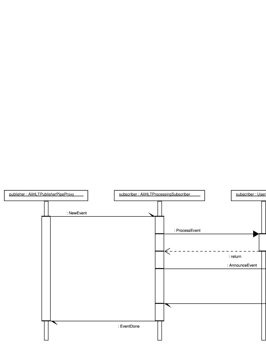
6.5.5 The Publisher Bridge Head Class
Like the two preceeding classes the AliHLTPublisherBridgeHead class is also designed to be used in cooperation with another class, the AliHLTSubscriberBridgeHead, introduced in section 6.6.3 and described in more detail in 7.1.4. Unlike the two other cases, however, the two bridge head classes are not situated in the same process, but instead each is present in its own process. In most cases these two processes will not even be running on the same node but on two separate nodes, as they together provide a transparent connection between components on different nodes. The connection mechanism as well as the publisher and subscriber bridge head classes are described more detailed in section 7.1.4.
6.6 The Subscriber Implementation Classes
Unlike the publisher classes there is no single basic implementation class at the root of the subscriber class hierarchy. An AliHLTSampleSubscriber class also exists but its functions are mainly just empty bodies. The only function that performs any action is the class’s Ping method that calls the calling publisher’s PingAck method as a response. The reason for this lack of a basic subscriber implementation is that unlike the publisher’s event and subscriber management and accounting there is little or no general overlap of functionality between the different subscriber classes. Therefore the AliHLTSampleSubscriber class is primarily a useful base class for subscribers that implement only some of the calls defined in the subscriber interface. Most of the subscriber classes are derived from AliHLTSubscriberInterface directly, rather than from an intermediate subscriber implementation class. Fig. 6.24 shows the class hierarchy for the three classes described in the following sections, including the subscriber interface and the sample subscriber class.
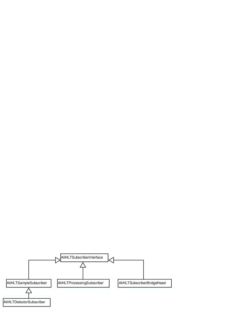
6.6.1 The Detector Subscriber Class
One of the classes derived from AliHLTSampleSubscriber is the AliHLTDetectorSubscriber class that was originally intended as the companion to the AliHLTDetectorPublisher class in 6.5.2. For the primary purpose as the subscriber object in data analysis programs of the type described in section 7.2, it has been superseded by the AliHLTProcessingSubscriber class described in the following section 6.6.2. This class provides a more advanced framework for receiving, processing, and reannouncing events. It reduces the additional tasks required for the writing of application specific programs to the implementation of one function. The detector subscriber class is still used as the receiving subscriber for a number of data flow components, like the event gathererer and scatterer programs presented in 7.1.
In the detector subscriber class three of the subscriber interface functions provided by the AliHLTSampleSubscriber are overwritten with additional functionality. The class also starts a thread for the class’s main processing loop, that uses a signal to wait for incoming events, prepares them, and calls the processing function for the event. This processing function is defined as an abstract method that has to be implemented by derived classes to provide actual processing functionality. Included in the preparation is a dereferencing step to convert the shared memory ID/offset combination for each data block into an actual C pointer passed to the processing function. When events are cancelled before they reach the processing step they are removed from the queue where they have been placed to be processed. For events cancelled while being processed, a flag is set that should be checked periodically in the processing function to avoid working on data that has been overwritten. Resources that have been allocated for these events are released after processing has finished or aborted. Events are added to the notification queue of the signal used in the main loop by the implementation of the NewEvent function.
6.6.2 The Processing Component Subscriber Class
The AliHLProcessingSubscriber class is the successor to the AliHLTDetectorSubscriber class. It is designed to be used as a subscriber object in either analysis components, with a subscriber and publisher, or in data sink components with only a subscriber for receiving data. For this purpose it implements all defined subscriber interface functions and starts two internal threads as well as a timer thread. Of these two internal threads one executes the class’s main processing loop while the other one contains a cleanup loop.
In the class’s NewEvent function the specified sub-event descriptor and trigger structures are copied. Pointers to these copies are added to the data queue of a signal object before it is triggered. In the main loop the processing subscriber waits for this signal to be triggered and as soon as this happens, it retrieves these two event meta-data pointers from the signal’s queue and prepares them for processing. As for the detector subscriber from the previous section this preparation includes the conversion of the shared memory ID/block offset pairs into pointers to each data block in the event. Unlike in the detector subscriber, a memory block for output data is also obtained from attached buffer manager and shared memory objects. The prepared and dereferenced block descriptors as well as the output memory block are used in the call to the event processing function, which again is defined as an abstract function that has to be overwritten by derived classes. If this function completes processing successfully and produces new output data in the output shared memory, and if the object is part of an analysis component and not a data sink, a sub-event descriptor is built for this data and announced via an associated AliHLTProcessingRePublisher object (cf. section 6.5.4) to any interested subscriber. For subscribers in data sink components event done data produced by the processing function is used to send the event done message to the event’s originating publisher. In analysis components a flag decides when an event done message is sent to the originating publisher, either when the event has been processed and new output data produced, similar to the data sink case, or when the associated republisher object informs the subscriber that the produced event data has been released by its subscribers. In the latter case event done messages will propagate back through a whole processing chain from the last processing component. Any event done data produced by the processing function is stored in this case with the event’s other meta-data and is attached to the event done data that has been received from the republisher’s attached subscribers. This assembled event done data is then used in the event done message sent to the event’s originating subscriber. Fig. 6.25 and Fig. 6.26 show sequence diagrams of the two cases for sending an event done message back to the originating publisher. To prevent event losses in the system the main loop contains error detection logic at each stage of the preparation, processing, and announcing steps. This is coupled with retry handling that ensures that an event with an error occuring anywhere in the stages is processed until it succeeds or until a permanent unresolvable error occurs.
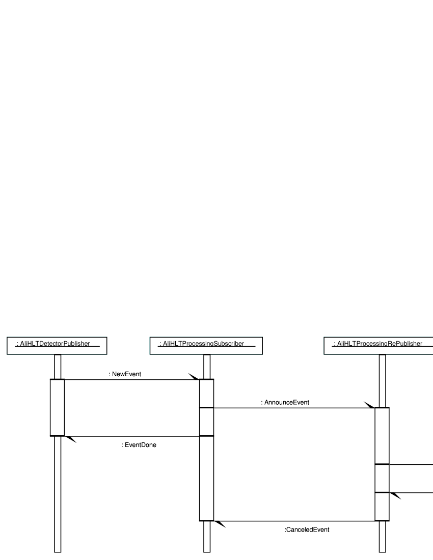
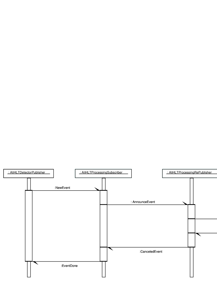
When an event is ready to be freed, any blocks reserved for its output data are released and a pointer to its event done data is placed into the queue of a further signal object. The subsequent triggering of this signal causes the cleanup loop running in the second thread to be activated. In this loop, the EventDone call to the event’s publisher is made using the assembled event done data. In addition, the event’s meta-data is removed from the internal structures of the object and further cleanup is performed as needed.
6.6.3 The Subscriber Bridge Head Class
At the sending end of a data bridge to an AliHLTPublisherBridgeHead object from section 6.5.5 and 7.1.4 is an instance of the AliHLTSubscriberBridgeHead class implementing the subscriber interface functions. This class is described in more detail in section 7.1.4 together with the other classes used in the bridging components.
Chapter 7 The Framework Components
Based upon the publisher-subscriber interface classes described in the previous chapter, a number of software components and component templates have been developed as the main part of the framework to allow the construction of complex data flow chains in PC cluster systems. The components can be separated by their purpose into several categories described in the following sections. For the configuration of the data flow in such a system a set of fully functional components exists, which are described in section 7.1. Section 7.2 details a number of template programs without actual functionality, whose purpose it is to ease the writing of components for specific tasks. Templates are provided for data sink, source, and processing components. Several worker components to create, modify, or otherwise process event data, some based upon these templates, are described in the following sections 7.3 to 7.4. The second of these includes analysis components which have been written for use in the ALICE HLT or its prototypes. The final section 7.5 contains descriptions of components dedicated to ensuring the fault tolerance of systems created using this framework. They function in conjunction with components from 7.1.
For the program components described below, a number of additional classes and functions beyond the interface classes described in chapter 6, have been written that contain some of their key functionality. These classes are described where appropriate.
7.1 Data Flow Components
The components described below are intended to configure the flow of data in a system constructed using the framework. Amongst others, components exist to merge parts belonging to the same event, to connect components on different computers, and to split up and rejoin a stream of events into multiple smaller event streams. None of these components modify the data specified by the event descriptors exchanged between the programs through the publisher-subscriber interface. Some modify the descriptors while they are forwarded unchanged by others.
7.1.1 Event Merger Component
Since multiple data sources may exist that produce data blocks belonging to one event, the EventMerger component exists to merge the multiple event descriptors for these parts into a single descriptor containing all blocks. For this purpose the program uses multiple subscribers, derived from the class AliHLTDetectorSubscriber, to receive the event parts. One output publisher, derived from AliHLTDetectorRePublisher, is used to announce merged descriptors. The component’s main functionality is contained in an object of the AliHLTEventMerger class to which the subscriber objects forward received events. Fully merged events are passed to the republisher object for announcement to attached consumer components. Fig. 7.1 and 7.2 show the relation of the classes in the component and a sample calling sequence of these classes respectively. The subscriber and publisher classes do not contain any significant functionality beyond calling the merger class’s corresponding functions.
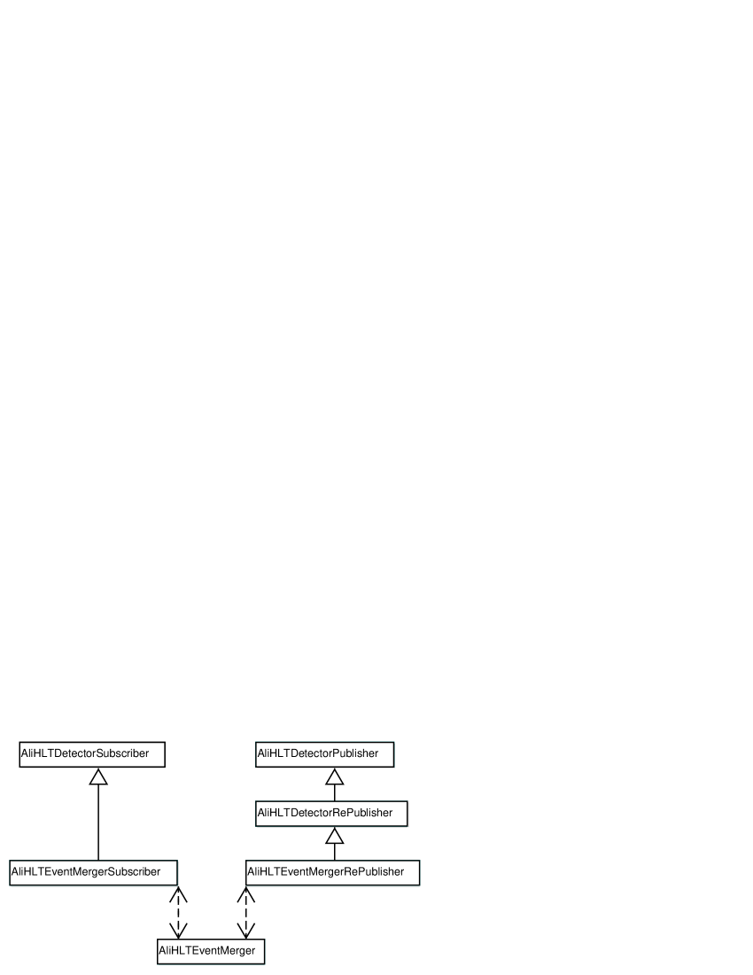
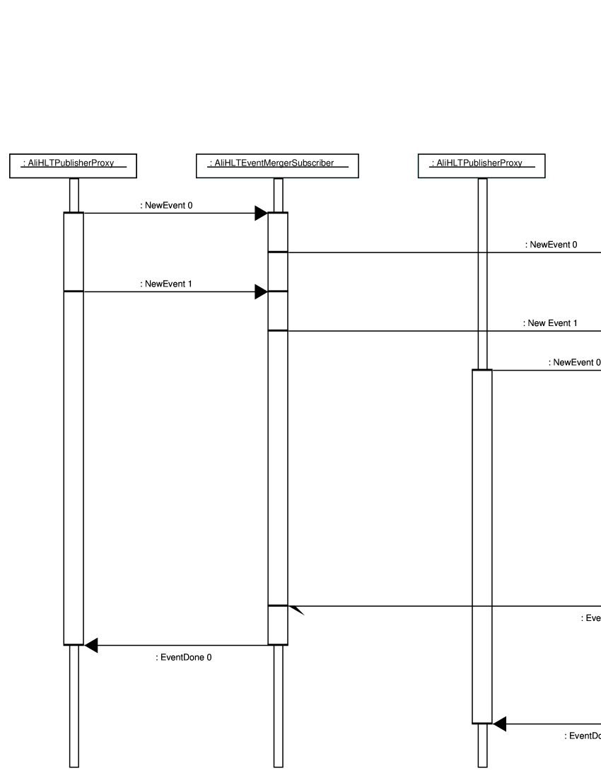
In addition to the component’s main thread, one thread is started as a subscription thread for the republisher object. One more thread is started for the message loop for each configured subscriber in addition to the two cleanup and processing threads started internally by each AliHLTDetectorSubscriber instance. In the program’s main thread a loop is entered that waits for all parts of an event to be completely received after which the assembled event is announced again. A timeout is configurable that will cause events to be announced when one or more parts were not received within a specified amount of time.
The Event Merger Class
The two main parts of the AliHLTEventMerger class are its list of configured input subscribers and the list for partially received and unannounced events. Of these two the subscriber list is the more simple one. It just stores pointers to the configured subscriber objects of the AliHLTEventMergerSubscriber class. Among the four most important elements stored in the event list structures are the number of contributing subscribers expected for this event as well as the number of subscribers from which parts have already been received. In addition, the event trigger structure from the first received subevent is also stored for each event. Another possibility might be to concatenate the event trigger structures from all event parts for the event’s reannouncement. The fourth important element of these structures is a list of descriptors for each data block contained in the received subevents.
When an event part is received by one of the configured subscribers, the event list is checked whether an entry for that particular event already exists. If no existing entry can be found, a new one is created with the event trigger data that has been received for this part, otherwise the existing entry is used. In both cases the number of subscribers from which data has already been received is increased, and the block descriptions contained in the received sub-event descriptor are added to the event’s data block list. As soon as the number of received sub-events is equal to the number of configured subscribers, the list entry for the event concerned is placed into a signal object. The subsequent triggering of this signal object activates the merger components’s main thread to retrieve the block list from the event data structure. A new event descriptor for the aggregated list will be constructed and announced through the republisher object in the program. During these steps the event data will not be removed from the event data list. It is kept in the list until the republisher object declares that the event has been cancelled through its appropriate callback function. When the specified timeout expires, the event list is also searched for the triggered event. If it is found, the event’s data structure will be signalled to the main thread as well, irrespective of the number of sub-events that have been received so far.
After the republisher has released an event, it informs the AliHLTEventMerger object by calling its EventDone method. The merger object searches for the event in its event list. If it is found it is removed, and all used resources are freed. Finally, an EventDone message is sent to all upstream publishers the merger component is subscribed to, allowing them to release the event as well.
7.1.2 Event Scatterer Component
One CPU executing one analysis component will not always be sufficient to alone perform a specific processing step of a chain at the required rate. The processing load of the steps concerned will thus have to be distributed among a number of CPUs. To provide this functionality in the framework the EventScatterer component has been created, which splits up an incoming stream of sub-events into multiple streams consisting of correspondingly lower rate of sub-events. Splitting of the stream is executed on an event-by-event basis, distributing whole events, and not by splitting up data from one event. In a manner analogous to the EventMerger component, the EventScatterer component uses one input subscriber and multiple output republishers. The input subscriber is derived from AliHLTDetectorSubscriber and is used to receive the input event stream, while the output publishers derived from AliHLTDetectorRePublisher make the multiple output streams available to other components. Unlike in the case of the merger component the scatterer’s main functionality is not contained in one specific class to allow the possibility of different algorithms for the distribution of the incoming events. The scatterer base class AliHLTEventScatterer has been defined to provide parts of the required functionality together with a number of callback functions that define an interface for scatterer classes to be used in the scatterer component. Currently only one derived class, AliHLTRoundRobinEventScatterer, is implemented for use in this component together with one class for use in the fault tolerance scatterer described below in section 7.5.6. It uses a simple round-robin algorithm for the distribution of the events among the configured output publishers. Neither the subscriber nor the republisher classes provide significant additional functionality beyond interfacing with the central scatterer object.
In addition to the program’s main thread and the two threads started by each subscriber, one subscription loop thread is started for each republisher object. In the main thread the subscriber’s message communication loop for the publisher-subscriber interface is executed. As soon as this message loops ends the scatterer component will be terminated as well. Fig. 7.3 and Fig. 7.4 show the relationship of the different classes in the scatterer and a sample calling sequence respectively.
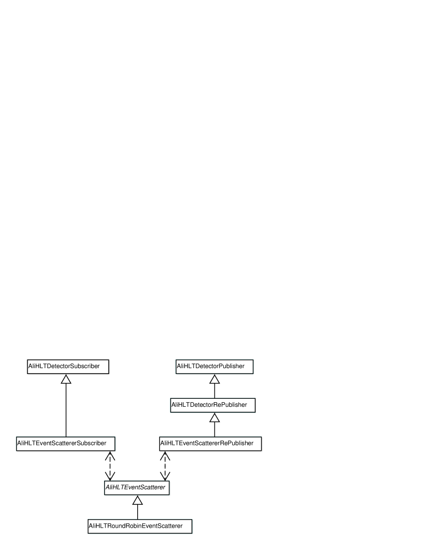
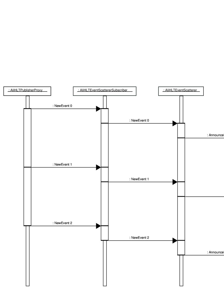
The Event Scatterer Base Class
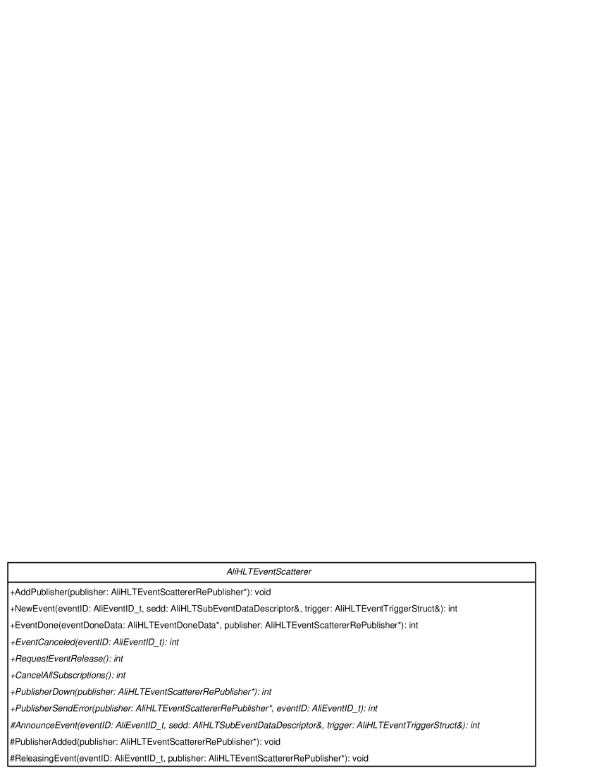
Internally the AliHLTEventScatterer class mainly consists of the list of output publishers which have been configured to be used. The interface functions it provides and defines are shown in Fig. 7.5. Among these are three main functions for use by programs, derived base classes, and its related subscriber and republisher classes: AddPublisher, NewEvent, and EventDone. The first of these, AddPublisher, has to be called to add an output publisher to a scatterer object to make its part of the received data available. It has to be called during the initialization of the scatterer component in its main thread and calls the PublisherAdded callback with the publisher object that has been added. The next of these functions, NewEvent, is called by the AliHLTEventScattererSubscriber object when a new event is received. EventDone on the other hand is called by one of the AliHLTEventScattererRePublisher objects when an event is released. Both of these functions call a further function declared or defined by this class. NewEvent calls the abstract function AnnounceEvent to dispatch an event to one of the available publishers to be announced, and EventDone calls the empty ReleasingEvent notification callback. Following this notification call, EventDone calls the EventDone method of the AliHLTEventScattererSubscriber object to allow the event to be released in its originating producer.
Among the six defined abstract methods in the AliHLTEventScatterer class three are public methods which are called directly by the subscriber object in the component. Two more public methods are provided for the case of publisher errors in the component. The final one is called internally by the class’s NewEvent method. There are two public abstract methods, EventCanceled and RequestEventRelease, called by the subscriber object when a particular event has been cancelled or when a request to release events has been received respectively. CancelAllSubscriptions, the third of these methods, is called when the subscriber’s own subscription has been terminated by its publisher. The two publisher error methods are called PublisherDown and PublisherSendError. PublisherDown is called from outside the class, either by a republisher object or by an external supervising instance, in response to a non-trivial error. Its purpose is to mark that publisher as unavailable, preventing the scatterer from sending any data to it. In contrast PublisherSendError is called whenever an error occured announcing an event for a specific publisher object. This is not considered a severe error and does not necessitate the removal of the publisher concerned. The final abstract method AnnounceEvent is the central method for each scatterer class. It is called by NewEvent whenever a new event is received to determine to which output publisher an event is dispatched for publishing. This is handled according to each scatterer type’s specific algorithm.
The Round-Robin Event Scatterer Class
In the basic EventScatterer component the AliHLTEventScatterer interface implementation is provided by its derived class AliHLTRoundRobinEventScatterer. It provides implementations of the six abstract methods defined in the base class. It neither overrides the default behaviour of other base class methods, nor does it implement any of the two callback methods provided by the base class.
A simple round-robin algorithm is used by the central AnnounceEvent method to select an output publisher for each event. To ensure consistency for multiple parts of an event passing through different parts of a system, this algorithm is not based on the event sequence number but uses an event’s ID instead. The same algorithm is also used by the implementation of the EventCanceled method to determine the republisher to which the notification about an event’s cancelation has to be forwarded. RequestEventRelease just forwards the release request to all publishers and CancelAllSubscriptions cancels all publishers’ subscriptions. Empty implementations without any functionality are provided for the two publisher error notification functions, effectively disabling handling of errors occuring in one of the scatterer’s publishers.
7.1.3 Event Gatherer Component
Most event streams that have been split up with the help of the EventScatterer component described in the previous section will have to be united into a single stream again at a later point of a data processing chain. This task is performed by the EventGatherer component, which can be seen as the inverse component to the scatterer, with multiple input subscribers and one output publisher in place of the scatterer’s multiple output publishers and single input subscriber. As for the merger component the subscribers’ class is derived from AliHLTDetectorSubscriber and the publisher’s is derived from AliHLTDetectorRePublisher. Fig. 7.6 shows the relationship of the classes used in the EventGatherer component. The merger and the gatherer components are very similar in their internal architecture. Their main difference is in the gatherer not having to receive one part of an event from each of its input subscribers. Instead it just has to forward each received event to its output publisher unchanged. Fig. 7.7 shows a sample sequence of events for this component.
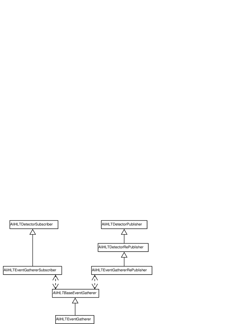
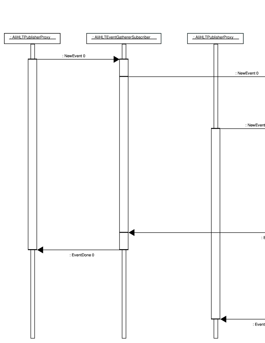
As in the EventScatterer component a base class, called AliHLTBaseEventGatherer, is used to define the central interface for the main gatherer class in the component with one data structure and five abstract methods. Actual gathering functionality is contained in a derived class AliHLTEventGatherer that provides implementations of these methods. As for the previous merger and scatterer components neither the subscriber nor the republisher component class contain significant functionality beyond the forwarding of function calls to the central gatherer object.
Internally, the gatherer’s primary data structures are its list of configured subscribers as well as a list of received and forwarded events which the ouput republisher could not yet release because they are still in use by at least one of its subscribers. This event list is necessary in the gatherer as it has to keep track of the event’s originating publishers, to be able to send EventDone messages for released events. In this respect it differs from the EventMerger, as that component receives parts of one event from each of the publishers it is attached to and thus has to send EventDone messages to each of them as well. Allocation and work task assignment for threads in the gatherer component is identical to the merger. One thread is started for each subscriber as the message loop for the publisher-subscriber interface communication plus each subscriber’s two internal threads for processing and cleanup. One further thread is created as a subscription request thread for the republisher object. In the component’s main thread a loop is entered that waits for received events to announce them via the republisher to any further components.
The Event Gatherer Base Class
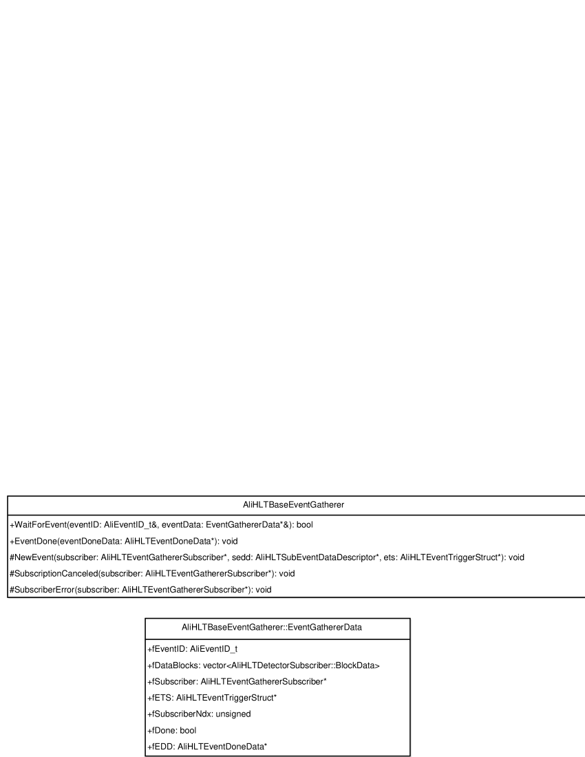
In the central gatherer object base class AliHLTBaseEventGatherer an interface is defined consisting of one structure data type and five abstract methods, both shown in Fig. 7.8. The EventGathererData type is used to store the data required to associate each event correctly with its originating subscriber. Primarily, this includes the event’s ID and the index number of and pointer to the originating subscriber object. Also available are an event’s trigger data as well as any event done data structures received for the event. These last two elements, however, are not used in the standard gatherer component. Finally, descriptors for the event’s datablocks are stored as well to construct a new subevent descriptor from them. This descriptor is used for the event’s announcement by the republisher object. Constructing a new subevent descriptor is necessary, as announcing runs in a separate thread from the receiving thread and the original descriptor may already have been released when the event is announced.
The abstract method WaitForEvent is intended to be called externally to wait for an event to arrive. In the EventGatherer component this is done in the program’s main thread. One further function, EventDone, is called by the component’s output publisher when an event has been released. Two of the remaining three functions, NewEvent and SubscriptionCanceled, are called by the subscribers configured for the component in response to a stimulus from the publisher they are subscribed to. The stimuli are either the arrival of a new event or respectively the cancellation of their subscription. The last function, SubscriberError, is called in response to an error that occurs in one of the specified subscribers, e.g. when attempting to send an event done notification back.
The Event Gatherer Class
In the class AliHLTEventGatherer, derived from the class AliHLTBaseEventGatherer, the two central data structures are a list of configured subscribers and a list of data structures of the base gatherer’s EventGathererData structures. The second list is used to store information about each event which has been received by one of the subscriber objects and announced through the republisher object, but is not yet released. Events are added to this list in the class’s implementation of the NewEvent function. In this function a pointer to the event data structure in this list is added as notification data to a signal object before it is triggered. A wait for this signal to be triggered is entered in WaitForEvent. Upon return from the wait the first available event structure in the notification data is returned to the function’s caller. In the EventGatherer component this caller is the function’s main thread, which uses this data to announce the event. When the provided implementation of the EventDone function is called by the republisher to signal a released event, the list is searched for the event concerned. If the event is found, its structure is removed from the list, and an event done message is sent to the subscriber from which the event has been received. A subscriber is removed from the object’s list of subscribers if its subscription is cancelled through the SubscriptionCanceled function. Each event that has been received through that subscriber subsequently has to be cancelled in all subscribers attached to the republisher as well. The final of the five abstract methods defined in the AliHLTBaseEventGatherer class, SubscriberError, is only implemented as an empty function body with no functionality. Subscriber error handling is not supported by this class and thus neither by the component.
7.1.4 Bridge Components
All components in the framework rely on the publisher-subscriber interface for communication between components. Due to the used mechanisms of named pipes and shared memory any communication in the framework is restricted to be local on one node. To lift this restriction and enable inter-node communication and data-exchange of components a set of two specialized bridging components has been developed. In the first, the SubscriberBridgeHead, data is accepted from a producer component and sent via a network to its partner component, the PublisherBridgeHead. The PublisherBridgeHead places the received data in a shared memory segment and announces it via its publisher object to further components subscribed to it. Fig. 7.9 shows the relation of the different publisher-subscriber and communication classes in these two components. A sample of the calls that occur between the classes in the components is displayed in Fig. 7.10. Using the standard subscriber and publisher interface objects for receiving and reannouncing data supports transparent connections of other remote framework components without special measures required in any of them.
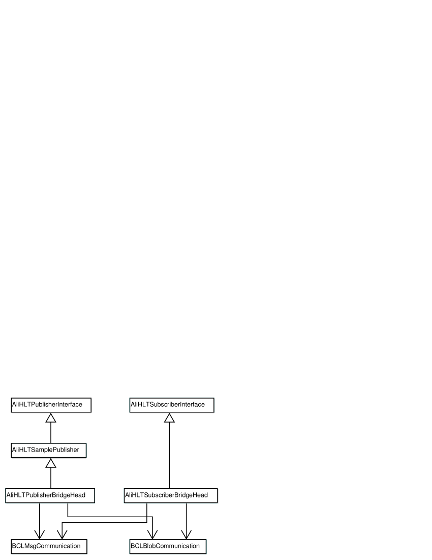
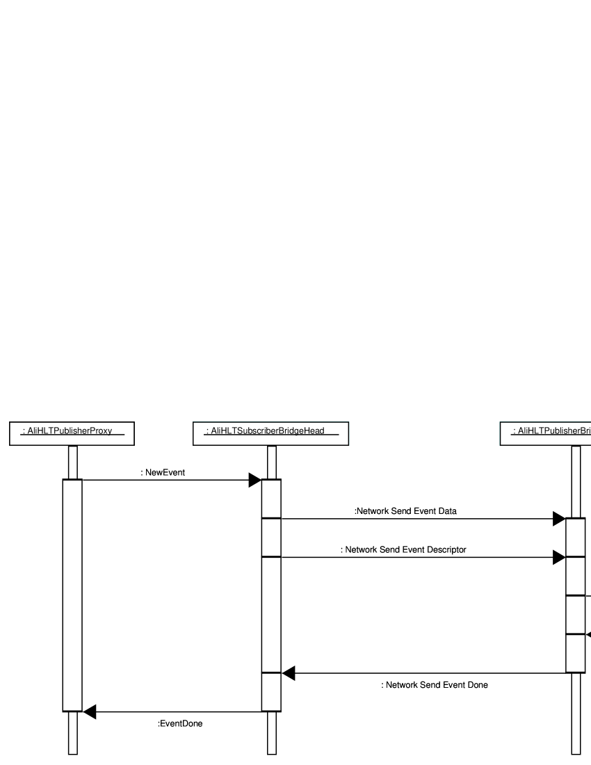
In the SubscriberBridgeHead component the major part of the functionality is provided by an instance of the AliHLTSubscriberBridgeHead class together with two instances of classes derived from the BCLMsgCommunication class and one instance of a BCLBlobCommunication derived class, all three described in section 5.4.1. Of these communication classes one message class object is used for the application level communication between the two bridge components, and the second message object is used for the required communication between the blob objects in the two components. Internally the SubscriberBridgeHead uses two threads in addition to its main thread and any background threads that may be created internally by the different communication classes. In the main thread the message loop responsible for the publisher-subscriber interface communication is run. The first additional thread is used for the network message loop that accepts and handles network messages received from the remote PublisherBridgeHead component. In the third thread the transfer loop for events is run that receives sub-events from the subscription loop through a signal object, accesses their data, and sends it over the network to the PublisherBridgeHead together with the parts of the sub-events’ descriptors necessary to announce the event. The class uses the approach of reserving the whole receive blob buffer and performing buffer management on it locally, as described in section 5.2.3. Local buffer management in the SubscriberBridgeHead is possible as each PublisherBridgeHead component receives its data from only one SubscriberBridgeHead, which thus can use the receive buffer exclusively. This approach has been chosen to minimize the number of messages exchanged between the two components and thus reduce the latency time needed to transfer an event.
On the receiving side the primary constituents of the PublisherBridgeHead component are an instance of the AliHLTPublisherBridgeHead class together with the same three communication class instances as in the SubscriberBridgeHead. The purposes of these communication objects are identical to the ones in the SubscriberBridgeHead: application level communication, blob message communication, and blob data transfer. Also similar to its sending counterpart, the PublisherBridgeHead uses two additional threads beyond the main thread and the threads started internally by its communication objects. One of the two additional threads executes the common loop for accepting new subscriptions for the publisher object while the other is the retry thread. This retry thread is responsible for trying to resend event done messages to the SubscriberBridgeHead where previous sending attempts for an event have been unsuccessful. In the program’s main thread the message loop to receive and handle network messages from the sending component is executed, similar to the message loop in the subscriber bridge head.
The Subscriber Bridge Head Class
The main data element of the AliHLTSubscriberBridgeHead class is a list of data structures for events that have been received from its publisher object. Pointers to the corresponding sub-event’s descriptor and trigger structures are stored in each event’s structure as well as a pointer to its originating publisher proxy object. Additionally, the number of retries that have been made to send the event to the publisher bridge head component are stored together with data about the event’s destination location in the receive buffer. This last information is required to release the part of the buffer used by that event, as the receive buffer’s management is performed in the sender component as described above. An event structure’s first three elements are the event descriptor, trigger structure, and publisher interface pointer. They are set when the event has been received from the publisher in the subscriber object’s NewEvent method before it is added to a signal object. This signal object is then triggered subsequently, to inform the transfer loop described below that a new event is available for sending. Buffer management data for an event is only set when the event’s block in the receive buffer has been successfully allocated, which takes place during the attempt to transfer it. The retry counter is increased every time a send attempt of the event to the remote partner fails. In addition to the event list the AliHLTSubscriberBridgeHead class stores pointers to the three BCL communication objects used for the network communication with the PublisherBridgeHead component. A pointer to the buffer manager object used for the receive buffer is also contained in the class.
Next to the functions implemented for the subscriber interface there are two functions that perform the major tasks of the subscriber bridge head class. In the MsgLoop function any messages received from the remote AliHLTPublisherBridgeHead partner object are handled. These are primarily connect and disconnect request messages as well as event done messages. Connection messages contain the addresses of the remote program message and blob message communication objects. If no connection is established, these addresses are extracted from the message and are used to establish a connection to the remote component. When a connection has been established successfully, the remote blob buffer size is queried, and the whole buffer is reserved as a transfer buffer for the events. The buffer size is also used to initialize the buffer manager object correctly. Events already stored in the object’s event list are now added again to the transfer loop signal object. After these additions the signal object is then triggered to activate the transfer loop. For disconnect requests not much action is required except for initiating the actual disconnection of the three communication objects. Received event done messages contain the event’s ID as well as any non-trivial event done data that has been received from the publisher bridge head object. This event done data is extracted from the message and is used to send an event done notification to the publisher that the component is subscribed to. Further actions in response to a received event done message include the cleanup of all object internal data related to that event, especially releasing the block occupied by the event in the buffer manager object.
The second main function of the AliHLTSubscriberBridgeHead class is the TransferLoop function, that is responsible for the transfer and announcement of an event and its data to the remote AliHLTPublisherBridgeHead object. In this function a wait is entered on a signal object triggered when new events are available for transfer, as described above. Available events are extracted from the signal object’s notification queue for processing. For each event a first check is performed whether a connection to the remote publisher bridge head is established, otherwise an attempt is made to establish one. If that connection attempt fails as well, the event transfer attempt is aborted. When a transfer is aborted the event concerned is entered into the object’s event retry list for a later send attempt. As soon as a connection is available, a block for the event data is allocated in the buffer manager. The event data is then transferred into this block in the remote receive buffer by the blob communication object’s multi-block transfer function described in section 5.4.1. After the successful transfer of the data an event descriptor message is constructed from the event’s original descriptor and the buffer manager data. This message is then sent to the remote component to announce the event. If the event has been cancelled by its originating publisher before the send process is complete, a special abort message is sent as the validity of the transferred event data cannot be assurred. Otherwise the announce message is sent normally and the event is kept in the list until the event done message for it is received from the publisher bridge head.
The Publisher Bridge Head Class
In the AliHLTPublisherBridgeHead class the two main data members are the list of events that have been received over the network from the subscriber bridge head and a retry list of released events for which the sending of the event done message to the remote AliHLTSubscriberBridgeHead object has failed. For each received event the sub-event data descriptor and the event trigger structure received from the sender component are stored in the event list. Each event’s done data obtained from attached subscribers is stored in the retry list. This data is sent in each attempt to the subscriber bridge head. In a retry loop failed event done data structures are attempted to be sent again when a retry timeout has expired. In addition to these two main data lists each AliHLTPublisherBridgeHead object also stores pointers to the three communication objects used.
Three of the functions from the callback interface provided for derived classes by the AliHLTSamplePublisher class are implemented in the publisher bridge head class: CanceledEvent, AnnouncedEvent, and GetAnnouncedEventData. Of these three functions AnnouncedEvent has a notification purpose only without actual functionality. GetAnnouncedEventData’s purpose is to obtain an event’s stored data descriptor and trigger structure for the reannouncement of events. CanceledEvent initiates the sending of released events’ done data to the AliHLTSubscriberBridgeHead.
Besides these three callback functions one further function, MsgLoop, contains the main functionality of this class. Similar to the subscriber class from the previous section, this function’s purpose is to receive network messages from its remote counterpart. The most important messages handled in this function are connection and disconnection requests as well as new event announcement messages. Connection request messages are handled somewhat in the same way as in the subscriber bridge head class. The address of the remote partner is extracted from the message, and then a connection to this component is established if it is not existing already. No send attempt of event done data accumulated before the connection is made, these attempts are only triggered by their respective timeouts, unlike for the subscriber bridge head’s event announcement sends. For disconnect requests the connection to the partner is simply aborted. NewEvent messages are the most complicated messages handled in the function. An event’s trigger structure and descriptor data are extracted from the message. The event trigger structure is subsequently used unchanged but the event descriptor is modified to use the correct shared memory segment ID, since this is not available in the sending component. When the correct data structures are assembled, they are added to the event data list and following this the event is announced by the component’s publisher to its subscribers.
7.1.5 Trigger Filter Component
One further functionality that has to be executed by a component is the triggered filtering of events. This means for the TriggeredFilter component that it has to receive events from a publisher and store them until a trigger decision for each is received. Based upon this trigger decision it determines which blocks of an event to forward and announces these blocks via its own publisher object to further subscribers. The mechanism by which the trigger data is received is the one provided by the SetEventDoneDataSend and EventDoneData functions, defined in the AliHLTPublisherInterface and AliHLTSubscriberInterface classes respectively. Trigger decisions are arrays of structures of the AliHLTTriggerDecisionBlock type described below.
Components that make the trigger decision for a particular event encapsulate vectors of these AliHLTTriggerDecisionBlock data structures into AliHLTEventDoneData structures. These structures are then transported back along the path that the event has been announced on. Components like the TriggeredFilter which have requested this will receive event done data originating from a publisher’s other subscribers. Each of the blocks in the trigger decision is then compared to an event’s data descriptor to determine which blocks are to be forwarded. Based upon this result a new event descriptor is constructed from the original one, and the event is announced to the filter’s subscribers. Fig. 7.11 shows a schematic sequence of events in the trigger filter component, a description of the classes follows below. For events where no block is selected through the received trigger decision two kinds of behaviour can be configured via command line options: Either the event concerned is not announced by the filter component at all or it can be announced as an empty event without any data blocks.
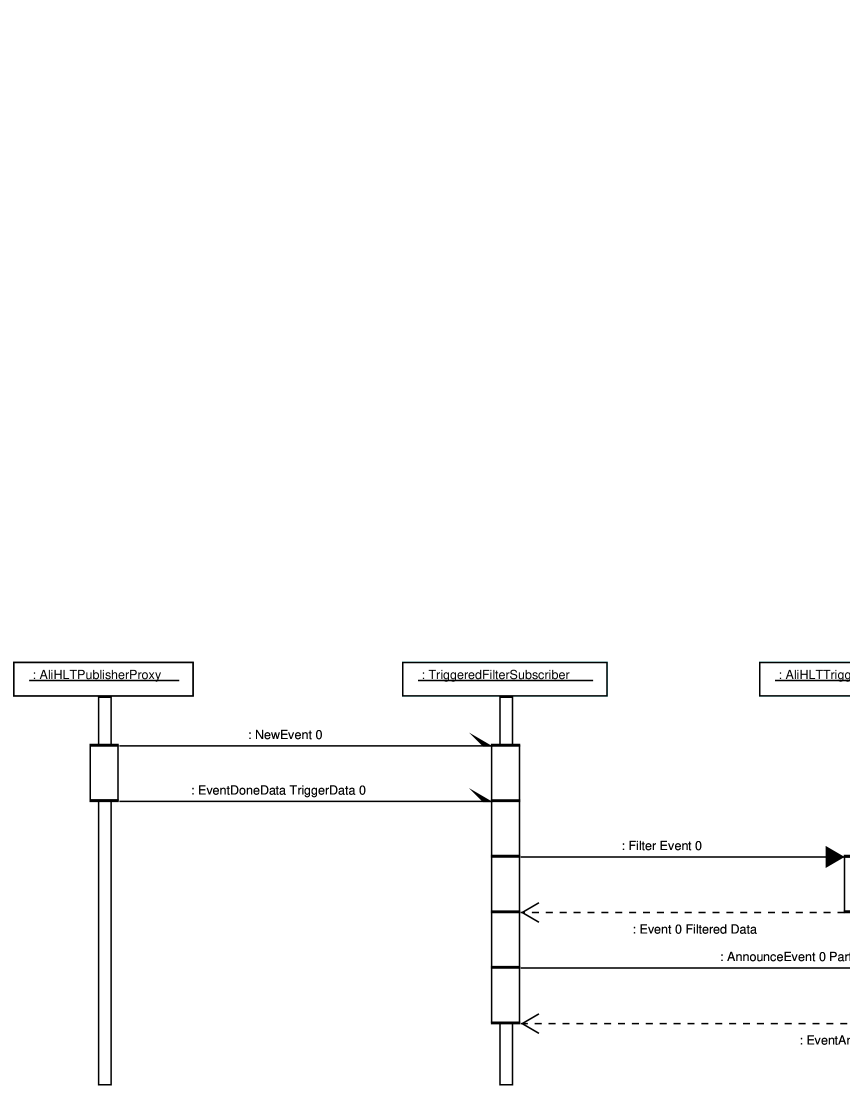
Internally the TriggeredFilter component consists of three main objects: a TriggeredFilterSubscriber object, a TriggeredFilterPublisher object, and an AliHLTTriggerEventFilter object. Its main logic is contained in the subscriber object which makes use of the event filter object for evaluating each event’s trigger data. The publisher object does not contain much functionality beyond the one provided by its AliHLTSamplePublisher base class. It starts a thread that contains the standard subscription loop and implements two of its base class’s callback functions, CanceledEvent and GetAnnouncedEventData. Calls to both functions are only forwarded to corresponding functions in the subscriber object. No threads apart from the mentioned subscription thread and those started internally by the AliHLTSamplePublisher class are started in this component. Fig. 7.12 shows the relation of the different classes in the component.
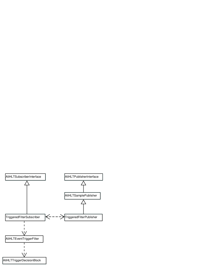
The Trigger Filter Subscriber Class
The TriggeredFilterSubscriber class contains the component’s main functionality. Its main data parts are two lists. One of them holds events that have been announced to the component, but for which no trigger decision has been sent so far and which thus have not been announced yet. The other contains the descriptors and trigger structures of events which have already been announced by the component’s own publisher and which have not been released yet. Both lists contain structures of the same type, storing an event’s descriptor and trigger data as well as a pointer to its originating publisher proxy.
The class’s functionality is contained primarily in the implementations of the NewEvent and EventDoneData subscriber interface functions. Supplementary functionality is contained in the subscriber interface function EventCanceled as well as in the CanceledEvent function called by the component’s publisher object. In the EventCanceled function the respective cancelled event is searched in the two event lists and is removed if found. If the event has already been announced through the component’s own publisher, it is aborted in the component itself, and the event cancelled message is forwarded to its subscribers as well. In the CanceledEvent function the event is also searched in the lists. If it is found, the event done data that has been received by the TriggeredFilterPublisher object is used in the EventDone call to the event’s originating publisher.
An event is added to the list of received events in the NewEvent function by placing copies of its descriptor and trigger data into the list. No further event processing or announcing is performed in this function as this only happens upon receipt of event done data from the event’s publisher in the EventDoneData function. When event done data is received, the trigger decision for the event concerned is extracted from it and the event is searched in the list of received events. The trigger decision data and the event descriptor are then passed to the AliHLTTriggerEventFilter object to appropriately filter the event’s descriptor. Depending on the results and the current setting the resulting descriptor is then used to announce the event through the component’s publisher to further subscribers. If the event is not announced any further, an event done message is sent to its originating publisher to release the event.
The Trigger Decision Block
Three data elements are contained in the AliHLTTriggerDecisionBlock structure that specify which data blocks of an event are to be read out: the block’s data type, its data origin and its data specification. These three fields directly correspond to the three fields of the same name and function in the AliHLTSubEventDataBlockDescriptor described in section 6.2.2 and are of the same respective type.
The Trigger Event Filter Class
In the AliHLTTriggerEventFilter class the main functionality is contained in the FilterEventDescriptor function. This function accepts an event’s data descriptor and a list of trigger decision blocks as its parameters. The trigger decision blocks are used to filter the data blocks from the event descriptor to be forwarded according to the trigger decision. Upon return from this function the event descriptor only contains those blocks that have not been filtered out so that it can be used directly to announce these events.
Matching of an event’s data blocks with the information in the trigger decision blocks is performed differently for the data type and origin and for the data specification field. For the type and origin a match is made if one of three conditions is met: The corresponding fields in the data block and the decision block are identical or one of the two fields contains the wildcard pattern of all 64 bit respectively 32 bit set. For the event data specification field matching modes are differentiated in the class by specifying a matching function in the filter object. Two predefined functions for this purpose are provided in the library. More matching modes are also possible by specifying user-defined matching functions instead of these predefined ones. In the first and simpler of the existing matching modes a match is found when the specification values from the descriptor and decision blocks are identical. This is similar to the matching for the data type and origin fields, although without the possibility for wildcards.
The second data specification matching mode is more complex and specific to the framework’s use in the ALICE High Level Trigger. It currently exists only as a first draft version and is still subject to modification. In this mode the data specification field is used to indicate an event data’s origin in the detector given in the data origin field. For data originating from the ALICE TPC the data specification contains the minimum and maximum numbers of the slice and patch specifiers as defined in section 2.2.2. If a data block’s specification overlaps with a decision block’s in both slice and patch numbers, then the block is marked for readout. All four fields (mininum and maximum slice and patch) in a trigger decision block are allowed to take the value of all 8 bit set, which corresponds to a wildcard for that number. Data originating from ALICE’s DiMuon arm contains the numbers of the DDLs used for readout of the data. A trigger decision block contains the minimum and maximum number of the DDLs to be read out for an event. For both the minimum and maximum DDL number for readout in the decision block 8 set bits again corresponds to a wildcard value for the number in that decision block.
7.2 Application Component Templates
To ease the programming of worker components for tasks other than those currently provided, three templates have been included in the framework. In general, application components can be divided into three types according to their position in a chain:
-
•
Data source components that obtain data from a source outside of the chain and make it available via a publisher object to other framework components. They are located at the beginning of a chain
-
•
Data processing components that receive data via a subscriber object, process it to produce some new output data, and make the new produced data available again from a publisher object. They are located in the middle of a chain.
-
•
Data sink components that receive data using a subscriber object and then either process the data and/or forward it to some destination outside of a framework chain. They are located at the end of a chain.
Fig. 7.13 shows the principle of the three application component types with their respective position in a chain. For each of these three types one template is present, written and commented to be adapted easily to a particular task at the intended position in a data processing chain. The following descriptions of the templates also contain instructions on how to proceed in adapting the templates to their intended tasks.
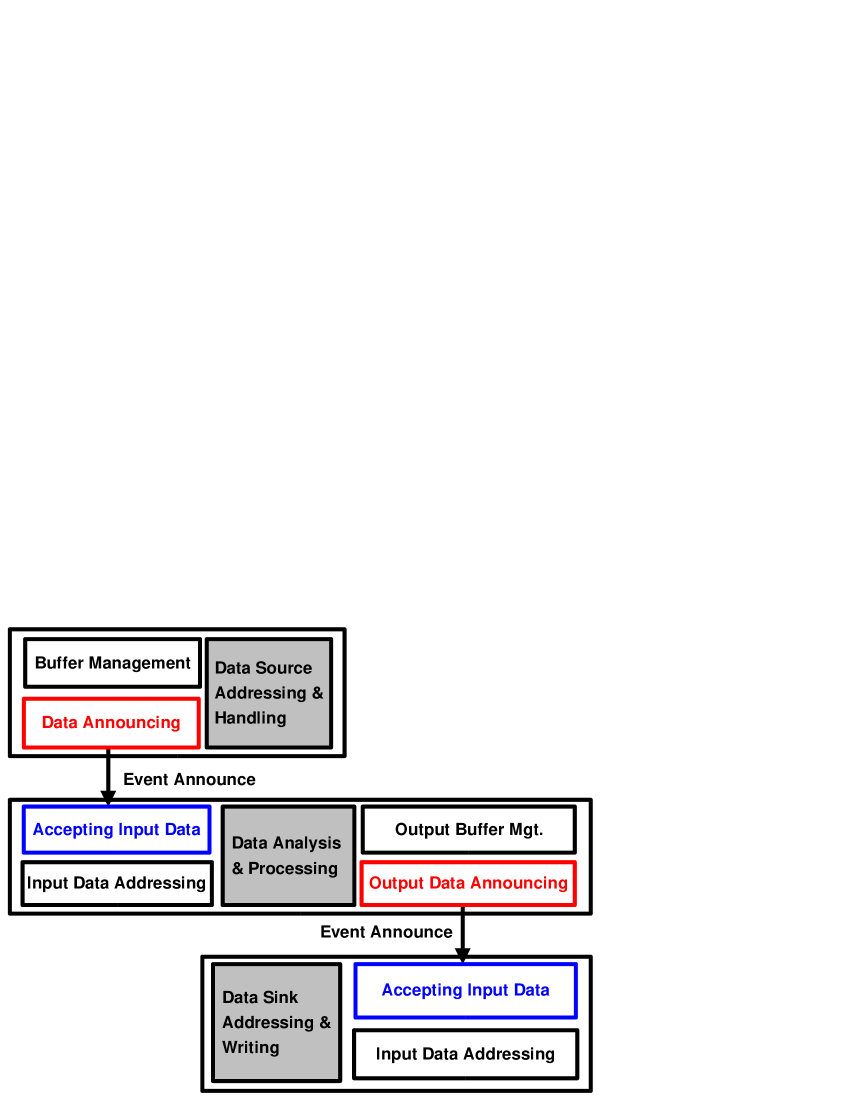
7.2.1 Data Source Template
Of the three component templates the data source component is the most complex one to implement due to the largest number of requirements and potential uses. The template is mainly intended for implementations that access a specialized readout hardware, e.g. in the form of a PCI card. Its main constituent part is an instance of a class derived from the AliHLTDetectorPublisher class described in 6.5.2. All six virtual functions defined in the detector publisher class are implemented by the template publisher class, although the functionality provided by the WaitForEvent method generates random data for publishing only. Functionality in the class’s other methods can be used as provided for software-only components that do not have to access hardware. An exception here are constants, like the block size for an event, which most likely differ for real tasks.
For data sources that have to access and communicate with special hardware devices more code will have to be added to the six detector publisher interface methods. In the WaitForEvent and EventFinished methods the functionality of the buffer manager object has to be replaced, if this task is performed already by the hardware. In this case a block in the output shared memory will not have to be allocated using the buffer manager in WaitForEvent. Instead the location of the data will have to be read out from the hardware. Similarly, in EventFinished the block will not have to be released in the buffer manager but the hardware has to be informed that it can now reuse the occupied memory. In StartEventLoop code has to be inserted to initialize the hardware device, while in EndEventLoop the device has to be deactivated. Finally, in QuitEventLoop an interface between the hardware and the component could be required to abort the event loop in WaitForEvent while it is still waiting for the device to provide information and/or data for a valid event.
7.2.2 Data Processor Template
In the data processing template two classes are used directly, one derived from AliHLTProcessingSubscriber described in 6.6.2 and one derived from the AliHLTProcessingComponent class described in more detail below. Only two functions have to be implemented in the AliHLTProcessingSubscriber derived class to be able to use the class in the template. The first of these functions is the class’s constructor, which has to supply required parameters to the base class’s constructor. Additional parameters that have to be passed to the new derived class can be added to those parameters as well. ProcessEvent is the second function that has to be implemented, defined as an abstract function in the AliHLTProcessingSubscriber class. It is called by the parent class when a new event is available for processing by the object. Input parameters to this function include structures containing the event’s data block descriptor with dereferenced pointers, the event’s trigger data, and a pointer to a preallocated output shared memory block as well as its size. Two primary output parameters of the function are a list of created output data blocks as well as a pointer to an event done data structure used in the EventDone message to the event’s originating publisher. In the function the input data blocks can be immediately accessed and processed. Output data can be placed directly into the provided output shared memory block.
For the class derived from AliHLTProcessingComponent two cases have to be distinguished, whether or not the processing subscriber class requires a set of parameters for its constructor different from the one for AliHLTProcessingSubscriber’s constructor. If the constructor parameters are identical for the two classes, a template class derived from AliHLTProcessingComponent can be used with the subscriber class’s name as the template parameter. This class contains an implementation of the abstract subscriber creation method described below, that supplies the default parameters to the constructor. To supply additional parameters required by the subscriber constructor a custom class has to be derived from AliHLTProcessingComponent that implements the abstract subscriber creation function with the necessary parameters. Both of these approaches are present in the sample data processor component, a #define statement selects one of them.
The Processing Component Class
AliHLTProcessingComponent is a complex class that encapsulates almost all functionality needed to set up a processing component. It parses the program’s command line parameters to extract necessary arguments and optional specifiers. Based upon these it creates all required objects and initializes them. Among the objects being created are cache classes for frequently needed data types, a buffer manager object, a republisher object, and objects for accessing shared memory. Creation of the subscriber class required for processing is not directly contained in the component class. Instead an abstract function, CreateSubscriber, is defined and called with the purpose of creating and returning a new subscriber object. This object must be of a class derived from AliHLTProcessingSubscriber to supply all functionality assumed by the component class. Also all necessary threads for the operation of a processing component are started so that amongst others the publisher’s subscription loop, the subscriber’s message handler loop, and a processing thread can operate without any further actions.
To make use of the functionalities of this class, a derived class has to be defined that implements the abstract CreateSubscriber function. For processing subscriber classes whose constructors do not require any special arguments the AliHLTDefaultProcessingComponent class can be used. This template class implements a subscriber creation function using the template parameter as the type of class to create with the processing subscriber default parameters. With a suitable derived processing component class available an object of that class has to be created with its required arguments in the component’s main function, and the class’s Run method has to be called to activate the processing component and start the processing of data.
7.2.3 Data Sink Template
The data sink template is very similar to the data processing component and uses the same two primary objects of classes derived from AliHLTProcessingSubscriber and AliHLTProcessingComponent. New events arriving are also handed to the user code in the ProcessEvent function that has to be implemented in the subscriber class. The difference between the two component types is attained by calling the NoRePublisher function of the AliHLTProcessingComponent derived class. This function specifies to the component class object that no republisher object is to be created, inhibiting the publishing of any produced data. Mostly, however, this component will not produce additional data but only perform a specific task with its received input data, e.g. writing to a file.
7.3 Generic Worker Components
In the following section a number of worker components are described not dedicated to a specific task of the framework. Most of them are intended to be used in debugging new components or chain setups, although they can also be used in small chains with limited functionality.
7.3.1 Random Trigger Decision Component
To aid in debugging the TriggerFilter component’s functionality, discussed in section 7.1.5, the AliRandomTriggerDecisionUnit component was created. It is a data sink component that does not process in any way the input data it receives. Instead it generates a random trigger decision consisting of multiple trigger decision blocks for each event. The generated trigger decision blocks are used as the event done data payload when the event is released.
For each of the generated trigger blocks one of the available block types is chosen at random. Seven trigger block types are available:
-
•
Empty or untriggered events
-
•
Completely triggered events
-
•
A specified TPC slice region, defined by a minimum and maximum slice number
-
•
A specified TPC patch region, defined by a minimum and maximum patch number
-
•
A specific type of data
-
•
A specific type of data in a certain TPC slice region
-
•
A specific type of data in a certain TPC patch region
If a block with one of the first trigger types is selected, no other decision block is allowed for the event concerned. The available datatypes as well as the valid slice and patch numbers are specified to the component via command line parameters. These parameters also allow to specify the trigger types to be used as well as a statistical weight for each of them.
7.3.2 Block Comparer Component
Testing the functionality of different paths in an event chain is the purpose of the BlockComparer component. This component will compare the data of all blocks in an event it receives and will provide a detailed report of the differences found. Its most simple and also most important application is to attach it to an event merger component with one input subscriber attached directly to an event’s originating publisher and the other to a publisher that publishes the same data after it has passed through a more complex chain setup of multiple components. If the data has been incorrectly transferred at one point of this chain, then the block comparer component will detect and report this error. Fig. 7.14 shows a sample setup of the principle. A publisher component announces data to a merger and a subscriber bridge head. From the subscriber bridge head the event data is sent via two publisher bridge heads and one subscriber bridge head to the second input subscriber of the merger. The merger announces the received events to the block comparer that compares their two blocks and thus can detect errors that have occured during the data’s transmission.
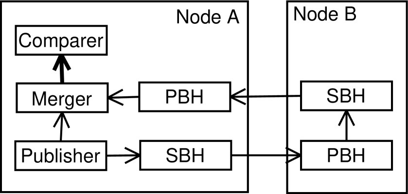
7.3.3 Event Dropper Component
By using the EventDropper component it is possible to test the behaviour of components and complete chain setups when events are lost in the system due to an error and are thus not released. This component is a very simple program with a subscriber object that sends EventDone messages back for most of its received events. Using a configurable rate, e.g. every hundredth event, the EventDone message is not sent at all and the event is just dropped. For the producing component to which the EventDropper is attached this means that the event will never be released by one of its subscribers and can only be removed when timeouts expire to force its release.
7.3.4 Event Keeper Component
In a manner similar to the event dropper, the EventKeeper component is designed to simulate the behaviour of components that require a specific amount of time to process events. It contains a subscriber object that starts a timer for each received event. When the timer expires an event done message is sent back to the event’s publisher. A constant amount of time to wait between the receiving of the event and its EventDone message can be specified via a command line parameter.
7.3.5 Event Supervisor Component
During the testing of components, especially in complex setups, events can become lost due to errors. Detection of such lost events is the task of the EventSupervisor component. It keeps track of every event received, and when a certain number of events has been received after a missing event a warning is issued. The number of events before the warning is configurable through command line parameters. If for instance the alarm intervall has been set to 50 and if event 100 is not received, an error will be reported when event 150 is received. Due to the fact that the component requires event IDs to be consecutive numbers, it cannot be used in configurations that encode other information in the ID.
7.3.6 File Publisher Component
In order to be able to simulate chains without having any special readout hardware available, a functionality was created to publish data contained in normal system files into a chain. The MultFilePublisher component reads data from multiple files and publishes events using that data. Each event contains data from one file. Files are alternated in a round-robin fashion. IDs of the events are numbered consecutively, starting with a configurable offset. The number of events to publish as well as the time interval to wait between the publishing of events can also be specified on the command line as well as the three data characteristics: type, origin, and specification.
In order to make the component more efficient, the data is read from the files directly into shared memory from which the events are published. This avoids file I/O and/or copy steps into shared memory for each event, reducing the CPU load. The component is mostly used in the simulation and testing of chain configurations without special readout hardware available.
7.3.7 Dummy Load Component
Simulation of chain setups without actual processing components is the purpose of the DummyLoad component based on the data processing template with AliHLTProcessingComponent and AliHLTProcessingSubscriber based classes. It simulates a processing component that receives input data and publishes new output data. To simulate different analysis components, a number of parameters in the DummyLoad can be configured via command line arguments. The most important of these parameters are the size of the output data and the simulated processing time for the data. Specification of the output data’s size is made as the percentage of the input data’s size, the value of this can be greater than 100 %, inflating the original data. Processing time can be specified in two ways, either as a constant value or proportional to the size of the input data. Similar to the file publisher component, it is also possible to specify the output data’s three characteristics type, origin, and specification.
Main parts of the component are two classes derived from AliHLTProcessingComponent and AliHLTProcessingSubscriber. The processing subscriber class implements the ProcessEvent method to copy the necessary amount of input data into the output shared memory and simulate processing for the specified amount of time. In the processing component class the main task is the evaluation of the additional command line arguments to extract the parameters that specify the simulation parameters.
7.3.8 Data Writer Component
Data that has been produced by components in a chain may be required to be stored permanently for later access. A very simple method for this is provided by the DataWriter component that creates a file using a configurable name prefix for each block in each event. Files are enumerated by the event’s ID and the block number in the event. For a large number of events this results in a correspondingly large number of files so that a periodic means of reducing the amount of files, e.g. by creating archives of events, becomes necessary. But for short and/or slow running setups this approach is sufficient.
7.3.9 Event Rate Component
The final generic worker component, the EventRateSubscriber, is a very simple data sink component. It receives events and immediately sends event done messages back to its publisher. After a configurable amount of events has been received, the component calculates the rate of events averaged over this number as well as the global average rate over all received events and prints these results to the logging system. This component is intended as a simple way to monitor the performance of a system in the absence of a more complete control and supervision system.
7.4 TPC Analysis Components for the ALICE High Level Trigger
There exist a number of analysis components ready to be used for the application of the framework in the ALICE High Level Trigger. Together these components allow to process run-length encoded ADC values, as read out from ALICE’s TPC, via space-points and tracklets to complete tracks of the whole TPC. After running a properly defined chain with these components the result is a completely reconstructed event of the whole TPC with all available particle tracks. The processing components in appropriate order are the ADC Unpacker, the ClusterFinder, the VertexFinder, the Tracker, optionally the patch internal track merger, the patch track merger, and the slice patch merger, all of which are described below. The analysis parts of these components have been written by collaborating partners from the University of Bergen, Norway [129], [130], [131], and have been integrated into the framework in Heidelberg.
7.4.1 The ADC Unpacker
The initial component in a processing chain for the ALICE TPC data is the ADCUnpacker component. It accepts input data in the form of zero-suppressed and run-length encoded ADC values as they are read out from one TPC patch. This data is uncompressed by filling in the suppressed zero values to create the component’s output data. During the uncompression process the data is inflated to about 2 to 3 times its previous size. Due to the fact that the data origin and specification fields in the event data block descriptor structures were not present at the creation of this component the slice and patch number that can be placed there for TPC data are not yet evaluated. Instead it is necessary to specify them using command line parameters. The slice and patch specifiers are placed at the beginning of the output data block together with the values for the minimum and maximum ADC padrows contained in the data so that the next components also have access to these numbers.
7.4.2 The Cluster Finder
Following the ADCUnpacker component and processing its output data is the ClusterFinder component. Using the unpacked ADC values, it calculates three-dimensional space coordinates of charge distributions, called clusters, produced in the TPC by the passage of charged particles. For each space point the produced output data contains the three cartesian coordinate values of the distribution’s center-of-gravity, the cluster’s width, and the amount of charge contained in it. The array of space points in the output data is preceeded by the originating data’s patch, slice numbers, as well as minimum and maximum numbers of the padrows read out. Additionally, the number of clusters found in the ADC values is also contained in this preceeding data block.
7.4.3 The Vertex Finder
One of two components that accept cluster data as its input is the VertexFinder component that uses the clusters from a slice’s outermost patch to provide a first calculation of an event’s reaction vertex position along the beampipe. It produces the cartesian coordinates of the determined vertex together with calculation error information for each coordinate. This is preceeded again by the first four numbers, patch, slice, minimum and maximum padrow number, extracted from the cluster data’s information block.
7.4.4 The Tracker
The Tracker component requires one or two input data blocks, cluster data from one patch, optionally together with the vertex data that has been calculated for the patch’s slice by the VertexFinder. When the vertex data is omitted, a central vertex position in the middle of the detector is assumed corresponding to the coordinates . Tracking is possible without vertex data although the result is more exact when it is available. The Tracker uses its input data to calculate segments of tracks, called tracklets, corresponding to paths of particles throught the TPC detector. Each tracklet is determined from the model of a helix, the path that charged particles follow in the TPC due to the magnetic field inside. The relevant parameters for this track model are stored for each found track. Among them are the center coordinates and radius of the helix when it is projected as a circle, the initial transverse momentum of the particle, as well as the start and end-point coordinates of the tracklet. Output track data is again preceeded by the patch, slice, and both padrow numbers as well as the number of tracks that have been found.
7.4.5 The Patch Internal Track Merger
The next step after tracking one patch’s data, the IntTrackMerger, is an optional component working on tracklet data from the Tracker. Multiple tracklets are merged into one tracklet, if their parameters are corresponding so that they belong to the same track. The output data format is identical to its input format as tracklets are read and produced. Due to this it is possible to insert this component transparently after a tracking component, although it is not mandatory. The following components cannot distinguish whether they work on data that was produced directly by the Tracker or by the IntTrackMerger. For high track densities the reduction in the number of tracks from one patch can speed up the following merging steps of multiple patches and slices.
7.4.6 The Patch Track Merger
Merging of the tracks of the six patches belonging to the same slice is the task of the PatchMerger component. It requires six blocks of tracklet data as its input, each block belonging to one patch. Using the tracklets from these patches the patch merger attempts to merge them across patch boundaries if they belong to a track with the same parameters. As its output the merger also produces tracklet data using the same track data structures as they are used for the output data of the tracker and patch internal track merger components. Unlike the previous components the patch merger’s output data is preceeded by only one of the four numbers, the slice number. As the ouput data does not belong to a patch subset but a whole slice, the other three numbers are not needed anymore. In addition to this location specifier the data is also preceeded by the number of tracklets contained in the following data section of the data block. Optionally, data from less than the slice’s full six patches can be merged. The number of patches on which to operate has to be specified as a command line argument. Missing patches in this case are assumed to contain no tracklets.
7.4.7 The Slice Track Merger
The last step in the TPC processing chain is the SliceMerger component that performs track merging using the tracklet data of multiple slices up to the TPC’s full number of 36. Tracklets are merged across the boundaries between adjacent slices to finally form full tracks passing through the whole detector. The format of the output data is still the same tracklet structure which contains all parameters to describe a full track as well. Preceeding the track array is just the number of tracks contained in the output data.
7.4.8 Future Steps
Following the final SliceMerger processing component the next required component is a trigger decision component. This component needs to analyse an event’s data to make a trigger decision to be passed back along the analysis chain through its event done data structure. The approach is similar to the AliRandomTriggerDecisionUnit component, although of course with a real analysis part to generate the trigger decision.
7.4.9 The Whole Chain
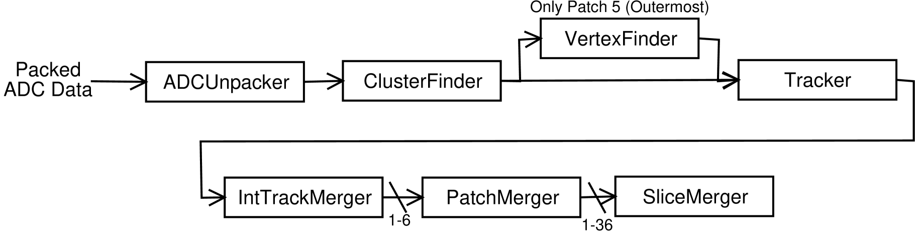
Fig. 7.15 shows a sketch of the sequence of data through the analysis components described in the preceeding sections. The vertex finder component only runs on the data of the outermost patch 5, although its output data, the vertex location, is used by all six trackers for the patches of the same slice.
7.5 Fault Tolerance Components
7.5.1 Framework Fault Tolerance Concept Overview
As has been pointed out in the introductory sections, a major challenge of the framework is the behaviour in case of errors, especially with respect to the intended operation of large clusters like the ALICE HLT. Errors can be single component failures on nodes or in extreme cases even failures of complete nodes, and both can be software or hardware related. Although the fault tolerance (FT) part of the EU DataGrid fabric management software [132] is intended to be responsible for the handling of errors concerning the system software and a node’s hardware, the HLT system still has to be able to react to node failures. This reaction as well as its triggering should work closely together with the GRID software framework.
In this section a set of components is presented that allows for such a reaction to the failure of any component in the system, which are handled on the granularity of complete nodes. On a failure the complete data stream to the node concerned is rerouted to other nodes and if possible a spare node is activated. The model is only applicable for data distributed by a scatterer to multiple nodes, one or more of which may fail, and is then collected again by a gatherer. In the current proof-of-concept implementation seven components are required: four data flow components, basically extensions of components described in section 7.1, one fault detection component, and two components that supervise and orchestrate the system’s reaction to the fault condition.
The four components extended with fault tolerance functionality are the Publisher- and SubscriberBridgeHead and the EventScatterer- and -Gatherer components, to form the TolerantPublisherBridgeHead, TolerantSubscriberBridgeHead, TolerantEventScatterer, and TolerantEventGatherer respectively. For the two bridge head components the added functionality is primarily the capability to perform remotely triggered connect and disconnect operations from their respective remote partners. The scatterer’s fault tolerant capability is to activate and deactivate output publisher paths, also remotely triggered. Similarly the gatherer is able to activate and deactivate its input subscribers for event done messages and to handle the case of multiple subscribers receiving the same event, which can happen if events are redistributed by a scatterer. In the following discussion of the components’ principles, a worker or spare worker node can also be a group of nodes connected together. One node in this group receives the data from the scatterer and passes it to the next one for processing, which continues until the last one sends its data to the gatherer. The two nodes connected to the scatterer and gatherer act as endpoints to the FT components.
ToleranceDetectionSubscriber, the fault detection component, basically consists of a simple subscriber object that receives events and immediately releases them again. For every event a retriggerable timer is started. The timeout used is configured by the command line. When the timer expires, indicating that no event has been received in that time, the detection component sets its own status accordingly and informs the first of the two supervising components of the status change.
In this supervision component, the ToleranceSupervisor, the status data of multiple fault detection subscriber components is checked regularly. When a change in the status of one of the subscribers is detected, the supervisor sends commands to the scatterer and gatherer components to deactivate the publishers and subscribers concerned. When an error is removed the publishers or subscribers can also be activated instead. After this a command is sent to the second supervision component, the BridgeToleranceManager.
In response to this message the bridge tolerance manager searches through its list of active and spare nodes and tries to activate a spare node if one is available. This activation is done by sending disconnect messages to the two bridge head components in contact with partners on the failed node. Once the disconnect is complete, another command is sent to the two bridge heads to reset their internal state by removing all event data left over from the severed connection. The reset step is necessary as the event data has already been resent to other nodes by the scatterer. Finally, a third command is sent to initiate a new connection to their new bridge head partners on the spare node. As soon as it detects this connection as established in the participating bridge heads, the bridge tolerance manager sends its final commands to the scatterer and gatherer components to reactivate their output publisher and input subscriber objects for the failed data path.
In a summary, the sequence of events is as follows:
-
1.
A node fails.
-
2.
The ToleranceDetectionSubscriber on a receiving node detects that no data arrives from the publisher bridge head connected to this node and sends a message to the ToleranceSupervisor.
-
3.
The ToleranceSupervisor checks the status of all configured ToleranceDetectionSubscribers and detects that the path between scatterer and gatherer containing the faulty node is broken.
-
4.
The ToleranceSupervisor sends messages to the TolerantEventScatterer and -Gatherer components on the sending and receiving nodes to disable the path concerned. A message is also sent to the BridgeToleranceManager to inform it of the failure.
-
5.
The scatterer and gatherer disable the path concerned. The Scatterer distributes all events that have been sent to that path and not received back among the remaining nodes. Incoming events for the failed path are also distributed among the remaining paths.
-
6.
The BridgeToleranceManager sends messages to the subscriber and publisher bridge heads on the sending and receiving nodes that communicate with the failed node, instructing them to disconnect from that node and to reset their internal state.
-
7.
Once the bridge heads are disconnected and reset the bridge tolerance manager determines an available spare node and sends commands to the bridge heads to connect to that node. (In a more complex real system it would also have to be ensured that the requires processes are available on the spare node. In this setup the worker and spare nodes are configured identically. )
-
8.
When this new connection is established on both sides the manager sends commands to the scatterer and gatherer components to reactivate the broken path.
-
9.
The status change of the path is detected by the path’s tolerance detector and the tolerance supervisor.
-
10.
The system functions normally as before, although with the number of available spare nodes reduced by one.

Fig. 7.16 shows the components in a sample setup using one data source and sink each, three processing or worker nodes, and one spare worker node. The ToleranceSupervisor and BridgeToleranceManager components can run on a separate node or on either the sink or source node.
For implementations that exceed this prototype a number of extensions to the above concept will be desirable or even necessary, mainly on the supervisor level of the concept. At least the two existing supervisor components, ToleranceSupervisor and BridgeToleranceManager, should be merged into one component. To avoid single points of failure in the system this supervisor component should exist in multiple instances in a system setup, with these instances ideally monitoring each other for failure. In addition the granularity of the system should be made finer, so that not only whole nodes can be replaced but also faults in single components can be recovered, e.g. by terminating and restarting the component and reattaching it to its communication partners.
7.5.2 Control and Monitoring Communication Classes
A central role in the fault tolerance functionality is taken by the classes that enable communication between a supervising and a supervised component. This is provided by two primary and a number of auxiliary classes, that together allow to send commands to supervised components and to query their status. An important characteristic supported by the classes is that supervised components are not purely passive but can also send interrupts, called LookAtMe or LAM, to supervising components to indicate a special condition. Of the primary classes AliHLTSCController is used in the supervisor and AliHLTSCInterface in the controlled component. Fig. 7.17 shows the six most important classes. The underlying mechanism used for communication between components by these classes are the BCL message communication classes. Communication is performed primarily without explicit connects, although supervisor initiated connections between components are possible as well.
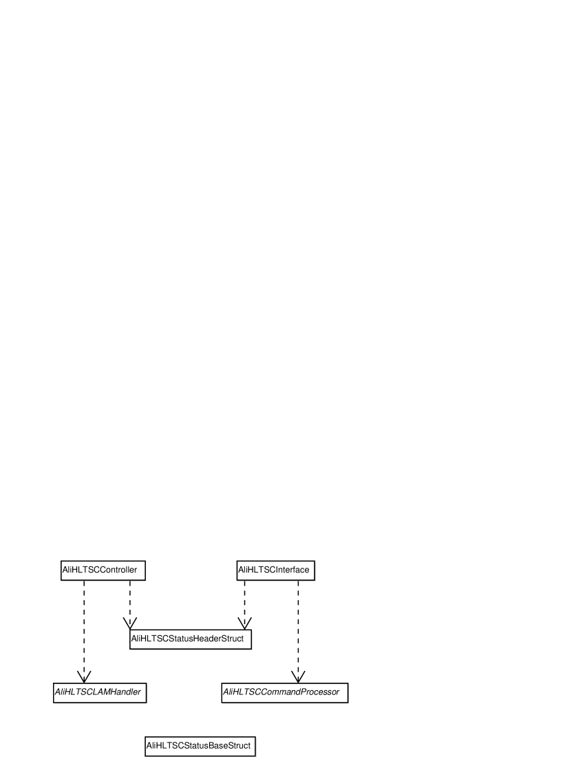
The Status Structures
Two datatypes exist that help to define structures used to hold status data for components, AliHLTSCStatusHeader and AliHLTSCStatusBase. The first of these structures basically is a container for structures derived from the second. As both are expected to be communicated over the network they make use of the data format translation mechanism defined in section 5.3.1. They are consequently derived from the BCLNetworkDataStruct type.
AliHLTSCStatusHeader contains three fields, a 64 bit long ID, the number of actual status structures it contains, and the offset in bytes of the first status structure, counted from the beginning of the status header. The ID field holds an identifier specific to the combination of status structures contained in the header structure. AliHLTSCStatusBase itself defines only two fields, another 64 bit long type ID and the offset of the following status structure in bytes, also counted from the beginning of the status header structure.
Actual structures containing status data are derived as vstdl types from AliHLTSCStatusBase and contain the status information as their fields. One example is the AliHLTSCProcessStatus structure which defines common status data for all components, like the current state and logging level of a process as well as the last update time of the status structure. This type is used as the first status structure contained in an AliHLTSCStatusHeader container by most components.
The Controlled Component Interface Class
The primary class used in supervised and controlled components is the AliHLTSCInterface class. It contains functions to provide a status header structure for readout by supervising components, to attach command processor objects handling received commands, and to send LAM messages to controllers. A number of commands are defined to be processed by the interface class itself, other commands are forwarded to the registered command processor classes. Internally the class uses two threads, one as the communication listening thread and the other for command processing. Its main data structures are pointers to the communication object with its local address, a list of addresses of connected supervisors, a pointer to the registered status header, and the list of registered command handler objects.
To use the class in the monitored component it first has to be bound to a listening address, to enable communication, and the two background threads have to be started using the Start function. Binding is done by calling the class’s Bind function, which accepts the local address and an error callback object as its parameters. The object’s local address is passed in the form of a string holding an address URL as defined in section 5.3.5. To release the bound address and stop the two threads the Unbind and Stop functions are used. Status data for a component is defined by specifying the address of the status header structure holding the component’s data to the class’s SetStatusData function. Status data can only be unset by passing a NULL pointer to the function.
For the handling of command processor objects two functions exist in the AliHLTSCInterface class. AddCommandProcessor adds an object to the list and DelCommandProcessor removes it. Both functions accept the pointer to the handler object to be added or removed as the only parameter. Command handler objects are described in more detail in the following section about the AliHLTSCCommandProcessor class. For LookAtMe notifications to supervising objects two functions exist as well, differing in their parameters and the intended receivers of the notifications. The first LookAtMe function sends the interrupt message to all supervisors that have established connections to this interface object, while the second version sends it to that supervisor object only whose address is specified as the function’s parameter.
The Command Processor Classes
Command processor objects are instances of classes derived from AliHLTSCCommandProcessor. This class just defines one abstract function, ProcessCmd. This function is called for registered handlers by their interface class instance when commands are received. The function receives as its only parameter the command structure that was sent by the controlling instance. Similar to the status structures the command structure AliHLTSCCommandStruct also makes use of the data translation mechanism and is thus derived from BCLNetworkDataStruct. It contains four fields: three 32 bit numbers holding the command itself as well as two parameters and a variable length array of 32 bit items. This array is available for holding additional required data which does not fit into the two numerical parameters.
The LookAtMe Handler Class
Similar to the command processor class, the AliHLTSCLAMHandler class is also an abstract class defining only one abstract function, LookAtMe. This function is called by the controller class for registered LAM handlers when a LAM request is received from a monitored component. The only parameter passed to the LookAtMe function is the address of the LAM’s originating component in the form of a BCL address structure
The Controller Class
The AliHLTSCController class is the main class to be used in supervising components, providing functions to register LAM handlers, establish connections to controlled components, and interact with supervised components. This interaction includes sending commands to, querying the status of, and setting the logging verbosity of components. Like the interface class described above the controller class also uses a BCL message communication object for communication with controlled components. One thread is used to receive and handle messages in this communication object. The class’s main data structures are a list of received messages that have to be handled, primarily replies from supervised components, the list of registered LAM handler objects, pointers to the communication object with its local address, and the address of a controlled object to which a connection has been established.
LAM handlers can be added or removed from a controller object using the two AddLAMHandler and DelLAMHandler functions respectively. Both functions require the pointer to the handler object to be added as their single parameter. As for the interface class, to be able to use an instance of this class its communication object first has to be bound to a valid address, and the background listening thread has to be started by calling the class’s Start function. Binding is performed analogous to the interface class by calling the Bind function with a string URL specifying the address and an optional error callback object as parameters. To release the bound address and stop the thread, the functions Unbind and Stop are available.
Once the controller object is ready, a connection can be established to one supervised component by calling the Connect function with the component’s address. Termination of a connection is achieved with the Disconnect function, also requiring the remote address as its parameter. All functions in the class that interact with a remote controlled component exist in two versions, one which requires the remote address of the component and one without an address. The second versions perform the corresponding task with the component to which the connection is established. If no connection is established they fail.
Three function pairs are available that operate on the remote controlled components. The first of these are the SetVerbosity functions that allow to set the logging verbosity as described in 4.2.1. As their only parameter, besides the remote address in one of the versions, they use the 32 bit large value for the verbosity, corresponding to the list of set flags for each verbosity level. This flag value is directly assigned to the global verbosity specifier in the remote component and takes effect immediately after it is received. Sending commands to remote components is the purpose of the second set of functions, called SendCommand, with the command to be sent as the only (additional) parameter. It is specified in the form of a pointer to the network transparent AliHLTSCCommandStruct structure passed to the command handler objects in the receiving components.
The final interaction function set consists of the two GetStatus functions for querying a remote component’s status data. They return a pointer reference to a status header structure containing the data that has been read out from the monitored component. Memory for the structure is allocated with the required size in the function when the reply message containing the status data is received. To release the allocated memory the FreeStatus function in the class has to be called.
7.5.3 Fault Tolerance Detection Subscriber
In the described situation a fault will be noticed first by the ToleranceDetectionSubscriber. This is a simple data sink component that notices when no events are received for a specified amount of time and signals an error condition to supervising components. Its internal main parts are a subscriber object of the ToleranceDetectionSubscriber class, a status data structure, and an instance of the AliHLTSCInterface class for communication with supervisor components. No threads are started explicitly by the component besides those started by its constituent objects.
In addition to its header two structure members are present in the component’s status data. The first of these is the common component status data, with the component type and status update time of main importance for the detection subscriber. Following this is an AliHLTSCToleranceDetectorStatus structure containing three fields specific to this component: the index of the path between scatterer and gatherer to which the subscriber is attached, the current state of the subscriber, and the ID of the last event that was received. A 32 bit unsigned integer is used as the state specifier field, holding either a 0 or a 1 for a faulty or functioning path respectively. The value contained in the path index field has to be specified to the component on its command line.
The Tolerance Detection Subscriber Class
As the primary class of the fault detection subscriber component the ToleranceDetectionSubscriber class is used. It is derived from the subscriber interface class and implements all its functions. Except for the NewEvent and Ping method all functions are implemented as empty function bodies only, without any functionality. In the Ping method the calling publisher’s PingAck function is called to acknowledge the received ping. The most important data structures in the class are the pointer to the component status structure and a list of supervisor addresses to which LookAtME messages are sent when an error is detected.
In the class’s NewEvent function the component’s status information is updated with the received information, including the timestamp, the event’s ID, and the state of the event path. If the component has not been paused as described below, a timer is set with a timeout value specified on the component’s command line. As the last action of the NewEvent function an event done message is sent back to the event’s originating publisher. When the timer started in the NewEvent function expires, then the class’s TimerExpired function is called. In this function the status data is updated by setting the last update time to the current time and the path’s state to faulty. Following this, a LookAtMe message is sent to each configured supervisor component address. Any error occuring during the send is ignored.
The last function of the class containing important functionality is the ProcessCmd function called when a command message is received for the component. Using these commands it is possible to initiate a paused mode for the component when no events are expected to arrive, to suppress raising of alarms. This pause state is necessary if the chain is still functioning, but the component delivering events to the fault detection subscriber cannot send events. Reasons for this might be errors in some readout hardware that have to be handled in a different manner or configuration changes in parts of the chain before this component.
7.5.4 Fault Tolerance Supervisor
As described above, the ToleranceSupervisor component is used as the location of the central supervising and decision making for the dataflow in a chain setup. When an interrupt is received from a fault tolerance detection component this component checks the state of all attached detection components to determine the status of the different data paths. A discovered faulty data path is removed from the active dataflow by sending the appropriate commands to the components responsible for routing the data. Similarly it is possible to reactivate a path once it has recovered from a fault.
Two primary classes are used in this component, ToleranceSupervisor and AliHLTSCController. Apart from any background threads started by the controller class and its internal communication classes, no further threads are started by the component. The controller object is used in the supervisor object to monitor and control the external detection and dataflow components.
The Tolerance Supervisor Class
Inside the ToleranceSupervisor class the primary data structures are lists for the detection and dataflow component addresses, the current and previous states and the last received event IDs of each detection component. Of these, the lists for the last event IDs, previous and current states have to be of the same size.
The main loop of the supervisor program is the class’s Supervise function that runs in a loop until a signal is caught to terminate the program. At the beginning of each loop iteration a wait is entered for the triggering of a signal object with a timeout of the interval between checks of the supervised detection components. A timeout is used in waiting so that asynchronous loop iterations outside of the fixed intervals are possible by triggering the signal object. Such a signal trigger is executed by the LAM handler function when an interrupt is received from a supervised component. When the signal’s wait function returns, the Check function is called to determine the channel state data from the configured detection and dataflow components. If a state change in one of the components is detected, pause commands are sent to all detection components, and the path concerned by the change is set to enabled or disabled accordingly by calling the class’s Set function. After these steps the next loop iteration is started.
Inside the Check function the status of each supervised component is read out using the supervisor’s controller class method GetStatus. Depending on whether or not a supervised component is a dataflow component or a tolerance detection subscriber, the channel state data in the status read is evaluated differently. For detection subscribers the read channel state is accepted to be the current state, while for dataflow components a channel state is only updated when the read state is faulty. This is necessary as the dataflow components have very little ability to determine a faulty channel state, particularly when the fault occurs on other nodes.
The first task in the class’s Set function is to send commands to the dataflow components, informing them that a specific monitored channel, or path, has been reported as faulty and should not be used anymore. After building the appropriate command structure, it is sent to all configured dataflow components. In addition the function sends another command to the configured bridge tolerance manager component. This component also has to be informed of the path’s failure, to terminate bridge connections to any nodes concerned and if possible activate a spare node replacing the failed one.
7.5.5 Bridge Fault Tolerance Manager
Complementing the fault tolerance supervisor component from the previous section is the BridgeToleranceManager component, that controls the bridge connections for the specific paths. To do so it maintains a list of required connections between data source, sink, and worker nodes for each of the paths. Additionally, it maintains a list of spare nodes in the form of available connection endpoints as well as lists of the supervised dataflow and detection subscriber components. The component contains two primary classes: BridgeConfig, responsible for reading and storing the configuration and providing access to its parameters, and CommandHandler, mainly responsible for communication with outside components. Outside components include the supervisor as well as the bridge, dataflow, and detection subscriber components. No threads are created by the component apart from those created implicitly by its objects, such as the controller and interface classes described in section 7.5.2.
In the component’s main function the command line options are evaluated first and the necessary objects are created, configured, and activated as needed. After this a loop is entered in which the component remains until it receives a signal to terminate. During each loop iteration two different types of status events with respect to the bridge components are checked. If a path has been deactivated and the bridge connections to its nodes have been terminated, new connections have to be established to a spare node, if there is one available. When these conditions are met, the bridge head components on the data source and sink node are checked whether the connections to the broken path have already been interrupted completely. This is necessary to ensure that the bridge heads have been able to reset their internal state and remove any old events from their internal lists. Once the connection termination has completed successfully, commands are sent to the sink and source bridge head components, containing the commands to connect to the corresponding partner components on the activated spare node(s).
The second check performed by the main loop is executed prior to the first check described above. When a reconnection attempt has been started it is necessary to periodically check the bridge components on the source and sink nodes whether the connection has been established successfully. If this the case, then commands are sent to the dataflow components responsible for routing the data to reactivate the path concerned. Once this is done, the broken path has been handled, and the system functions as before.
The Bridge Connection Configuration
A configuration for the bridge fault tolerance manager is described in a file using six different types of entries, with each entry consisting of one line:
-
1.
Data source entries describe connection parameters for a connection from the data source node to a worker node. Each of these connections is identified by a unique number corresponding to its path. To account for the fact that multiple data sources may be present, each entry also contains a subnumber. Entries with identical major numbers must have different subnumbers. They belong to one path which has multiple data sources that have to be merged in the path. The number of data source entries with the same major identifier and different subnumbers must be identical for each of the different source numbers.
Four parameters are specified for each data source entry: the control address URLs of the subscriber and publisher bridge head components as well as the message and blob-message address URLs of the publisher bridge head component. The subscriber bridge head component runs on the data source node, while the publisher bridge head runs on a worker node. It is not necessary here to specify the message and blob-message address URLs of the subscriber bridge head as they do not change, contrary to the worker node address which can change due to a node’s failure and replacement by a spare node.
Entry format (On one line):
’source’ <number> <subnumber> <subscriber-control-address-URL> \<publisher-control-address-URL> <publisher-msg-address-URL> \<publisher-blobmsg-address-URL> -
2.
Data sink entries describe the connection parameters for the opposite chain ends from a worker node to the data sink node. Each of these connections is also identified by a unique number which corresponds to the path that feeds the connection. Unlike the data source connections described previously, multiple data sink connections that belong to the same path are not supported. A one-to-one relation exists between a connection and a path, as it is assumed that data has been merged before it is sent to the sink node.
The parameters that have to be specified for a data sink entry are the control address URLs of the subscriber and publisher bridge heads as well as the message and blob-message address URLs of the subscriber bridge head, in analogy to the data source entry parameters. Here the subscriber bridge head component runs on the worker node while the publisher bridge head is located on the data sink node. Similar to the source entries’ subscriber bridge head message and blob-message address, it is not necessary to specify these addresses for the publisher bridge head, since they do not change either.
Entry format (On one line):
’sink’ <number> <publisher-control-address-URL> \<subscriber-control-address-URL> <subscriber-msg-address-URL> \<subscriber-blobmsg-address-URL> -
3.
Spare data source entries contain the worker node parameters required for the connection of a data source node to a specific spare worker node. A data source worker node is identified like a normal data source entry by a unique major number in combination with a subnumber. This number is located in the same address space as the numbers for the normal source entries and is thus not allowed to conflict with them. For each spare source entry the amount of subnumbers must also be identical to the one specified for the active source entries. Parameters that have to be specifed for a spare data source entry are the three parameters for the publisher bridge head in the source node to worker node connection: its control, message, and blob-message address URLs. It is not necessary to specify the control message of the subscriber bridge head on the source node as this is obtained from an active source entry when a connection is established to the spare node.
Entry format (On one line):
’sparesource’ <number> <subnumber> <publisher-control-address-URL> \<publisher-msg-address-URL> <publisher-blobmsg-address-URL> -
4.
Spare data sink entries are the analogue of the spare data source entries for the worker to data sink node connection. They are identified similarly to the normal data sink entries by a unique number, located in the same address space as the normal sink entries. Three parameters for the subscriber bridge head on the worker node have to be specified: the control, message, and blob-message address URLs. Analogous to the spare source entry the parameters for the publisher bridge head on the sink node do not have to be specified.
Entry format (On one line):
’sparesink’ <number> <subscriber-control-address-URL> \<subscriber-msg-address-URL> <subscriber-blobmsg-address-URL> -
5.
Target entries specify control address URLs of command targets to which command messages will be sent when a broken connection has been reestablished using a spare node. Such a message instructs the targets to reactivate the path that has failed. Typically, these are tolerant event scatterer and gatherer components controlling the data flow. The only parameter that needs to be specified here is the control address URL used by the target component concerned.
Entry format (On one line):
’target’ <target-control-address-URL> -
6.
Detector entries specify the fault detection subscriber components used for each path. A detection subscriber is identified by the number of the path it belongs to. The parameter that has to be specified for such a component is the control address URL used. Using these entries start commands are sent to detection subscribers when a faulty path is reactivated after a failed node has been replaced by a spare node. Reactivation is required as the detection subscriber has been paused by the fault tolerance supervisor when the fault occured.
Entry format (On one line):
’detector’ <nr> <tolerance-detector-control-address-URL>
The Bridge Configuration Class
Reading a configuration file, storing the read configuration, and providing easy access to its data is the task of the BridgeConfig class in the bridge tolerance manager component. To read a configuration the class’s ReadConfig function has to be called with the name of the file in which the configuration is stored. Access to the configuration data is provided by a number of member functions that return different parts of the configuration in a structured manner.
GetActivePath and GetPath return data about an active path or one path from the whole set of active and spare paths, respectively. In both cases the path is selected by the number specified in the configuration file. For active paths only entries specified by the data source and sink entries are searched, while for the whole set of paths the spare source and sink entries are searched as well. The information returned for a path includes the connection data for the data source connections and the data sink connection. There may be multiple data source connections between the configured number of sources and worker nodes, but only a single data sink connection between one worker and data sink node. Furthermore, the path’s absolute and active path numbers and the type of the path are contained in the returned data field as well. A path’s absolute and active number can differ, e.g. for spare nodes that have been activated. The type of a path specifies whether it is active or down or whether it is a spare path.
The class’s GetTargets function returns the list of address structures that have been specified in target component entries. GetToleranceDetector provides a structure for the fault detection subscriber component that has been configured for the path number specified to the function’s call. Included in the returned data is the control address URL under which the detection subscriber can be addressed.
Two functions are provided to set certain parameters of the configuration. The first of these, SetPathStatus, is used to set the state of a specific path in the stored configuration to either down or up. An active or spare path’s state can be set to down, while only a down path’s state can be set to up. When an active path is set to down, the list of spare paths is searched for an available path that can be used to replace the broken path. If a spare path is found, the control addresses of each data sources’s subscriber bridge head and of the data sink’s publisher bridge head are copied into the spare path’s data structure and reset in the original active path’s data. The original path’s active number is also copied into the spare path, and the states of the paths are set to down and active respectively. A spare path which is set to down triggers no further action, while a down path which is available is placed into the list of spare paths.
When a new spare node has just become available it can be used to reactivate a broken path by the SetSpareActive function called from the command handler class. This function searches for the path with the specified active number in the list of paths requiring replacement. It also searches the list of spares for an available path to be used as a replacement. If both an active path to be replaced and an available spare are found, the source subscriber bridge head’s and sink publisher bridge head’s control addresses are moved from the original path to the spare one. The active number of the new path is set according to the old active path’s one, and the new paths’ state is set to active.
The Bridge Command Handler Class
The CommandHandler class in the component is derived from the AliHLTSCCommandProcessor class described in section 7.5.2. Its ProcessCmd function is called by the controller object in the component when a command is received, its four other functions are called from the component’s main loop.
In the ProcessCmd function only the command to set a bridge node’s state is handled, which specifies a change in the state of a path in the system. The command is handled by interfacing with the component’s BridgeConfig instance. When a path is set to up or available an internal list of paths that need to be replaced is searched to determine whether a failed and unrecovered path exists. If such a path is found, it is placed into a list of paths that need to be connected to their source and sink node endpoints, using the spare path’s endpoints. The list of paths requiring reconnection can be queried by calling the class’s GetConnectsNeeded function. This is done in the component’s main loop, as described above.
For a path whose state is set to down, different steps are taken in the command processing function. First the path’s parameters are queried from the configuration object. Then three commands are sent to the bridge head components on the source and sink nodes belonging to the path: A disconnect command to abort the connection to the broken path, preceeded and followed by a purge events command to clear all events that have remained in these components. Following this, the path’s state is set to down, and a spare path to activate is searched. If no available spare path is found, the path is placed into the list of path’s that need to be replaced. The list is searched when a path becomes active again, as described above. Otherwise, if a spare path is available, it is activated in the configuration and placed in the command handler object’s list of connections that have to be established. This is the same list into which a newly activated path is placed when it has to replace a broken path (see above).
When the program’s main loop has retrieved a set of connections that have to be established, it calls the command handler’s MakeConnection function for each of them after the disconnection from their previous remote partners has completed. In this function connection command messages are assembled containing the message and blob-message addresses of the new bridge head components in the path to be activated. After these messages have been sent successfully to the bridge heads on the data source and sink nodes, the path is removed from the list of paths that have to be connected and placed into a list of paths to which reconnect commands have been sent. This second list can be queried by calling the class’s GetReconnectPaths function. In the main loop this function is called, and the states of all connections in the subscriber and publisher bridge head components of the path are queried. If all connections are established successfully, the command handler’s SetTarget function is called to reactivate the replaced path. In this function a start command is sent to the fault detection subscriber monitoring the path concerned. Further commands are sent to all configured target components to set the path’s state back to active, instructing the data flow components to send events to that path again.
7.5.6 Fault Tolerant Event Scatterer
One of the two components responsible for routing the dataflow in a fault tolerant chain setup, the TolerantEventScatterer component is an extension of the EventScatterer from section 7.1.2. It replaces the AliHLRoundRobinEventScatterer object in the original scatterer with an AliHLTTolerantRoundRobinEventScatterer object and adds a number of objects for the fault tolerance tasks in the component. Fig. 7.18 gives an overview of the most important classes used. The component’s main program does not differ significantly from the event scatterer’s. Major differences are the use of another central class and the configuration, creation, and setup of the required auxiliary objects for the FT tasks. Primarily, these are an instance of the AliHLTSCInterface class from section 7.5.2 and a status structure derived from the ones described in the same section.
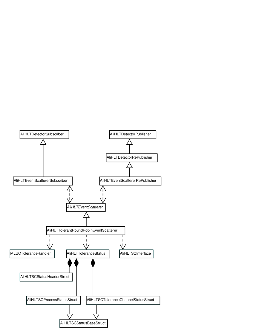
The Fault Tolerant Round Robin Event Scatterer Class
Similar to the original AliHLTRoundRobinEventScatterer class, the AliHLTTolerantRoundRobinEventScatterer class is also derived from the AliHLTEventScatterer class, described in section 7.1.2, implementing the six abstract functions defined by that class. It also overwrites the two callback functions provided by the base class. The main difference between the basic round-robin scatterer class and this class is that AliHLTTolerantRoundRobinEventScatterer uses an MLUCFaultToleranceHandler object, described in section 4.2.1. This object distributes the work load of events only between functional output publisher paths, taking into account their respective status. In addition, it is possible to control this class to a certain degree from external components via a control and monitoring interface class instance.
The primary data structures on which the class operates are lists of events, one for each of the configured output publishers and one for retry events. Events are entered into the retry list when all output publisher paths are marked as broken and no publisher is available to announce the event. An event is entered into a specific publisher’s list when it has been announced by that publisher. The data placed into each of the lists contains everything required to announce, or reannounce, the event: its ID, sub-event descriptor, and event trigger structure, plus the time at which it arrived. Storing this data in the component is necessary in case the event has to be reannounced due to a failure of the output path to which it was assigned.
Beyond these lists two auxiliary objects are used in the class as well as objects of two proxy classes. The proxy class objects function as forwarders between a command processor and the scatterer object on one hand and the scatterer object and an FT interface object, described in section 7.5.2, on the other hand. In the first case a function in the scatterer is called to handle received commands, while in the second LAM requests are forwarded from the scatterer to an interface object. The fault tolerance handler object is only used internally in the class, while the status structure is passed from the component’s main program and is just updated in the class.
Although all of the functions implemented in the class contain some code related to or affected by the fault tolerance functionality of the component, the most important work of correctly distributing the events is done in two functions: AnnounceEvent and SetPublisher. AnnounceEvent is called whenever a new event has to be announced to a publisher. The publisher to be used is first determined with the help of the fault tolerance handler object. When a publisher is found, the event is announced to it and is placed with the required data in the event list for that specific publisher. If no publisher could be found for the event, all publisher paths must be broken and the event is added to the list of retry events. The retry list is accessed when at least one publisher becomes available again. Events are removed from a publisher’s list when the event is released by the scatterer’s (re-)publisher or when it is cancelled by its original publisher from which the scatterer received it. In the first case an EventDone message is sent via the scatterer’s subscriber to the event’s originating publisher.
The second important new function, SetPublisher, is called by the command processor function when the state of one of the output publisher paths in the system changes. If events have to be announced or reannounced as a result of such a change, the function calls AnnounceEvent after updating the concerned publisher’s state. After a status change command has been received, a publisher with the given index is searched and its status in the fault tolerance handler is compared to the specified state. If these states are equal, the change has already been processed and the function performs no further action, otherwise the state is updated in the handler object.
When a publisher path has become functional again and the retry list contains events, these events are processed. They are removed from the retry list and passed to the AnnounceEvent function to be announced. If no events are contained in the retry list, the publisher is only used for the respective fraction of new incoming events. For a state change to non-functional the event list of the concerned publisher is accessed. Each event is removed and handed to the announce event function. Due to the status change in the fault tolerance handler object these events are assigned to a different, still functional, publisher able to process them. After these events have been reannounced, they are aborted in the faulty publisher to which they had been assigned originally, using the publisher’s AbortEvent function so that no event is contained in two publisher objects.
One more function contains functionality related to the fault tolerance operation. This is the PublisherDown method called by one of the scatterer’s republisher objects when an error occurs in one of its subscribers. In the function the state field in the status data structure corresponding to this publisher’s state is set to faulty, and a LookAtMe request is sent to a supervising component. The decision to remove this publisher’s path is not taken locally in this component but instead in the supervisor component when it has checked the respective state.
7.5.7 Fault Tolerant Event Gatherer
The second component responsible for routing the dataflow in a fault tolerant chain setup is the TolerantEventGatherer component, an extension of the EventGatherer component from section 7.1.3. Similar to the fault tolerant event scatterer component, this component replaces the AliHLTEventGatherer class from the original gatherer with the extended AliHLTTolerantEventGatherer class and adds a number of additional helper objects. Fig. 7.19 gives an overview of the most important classes used.
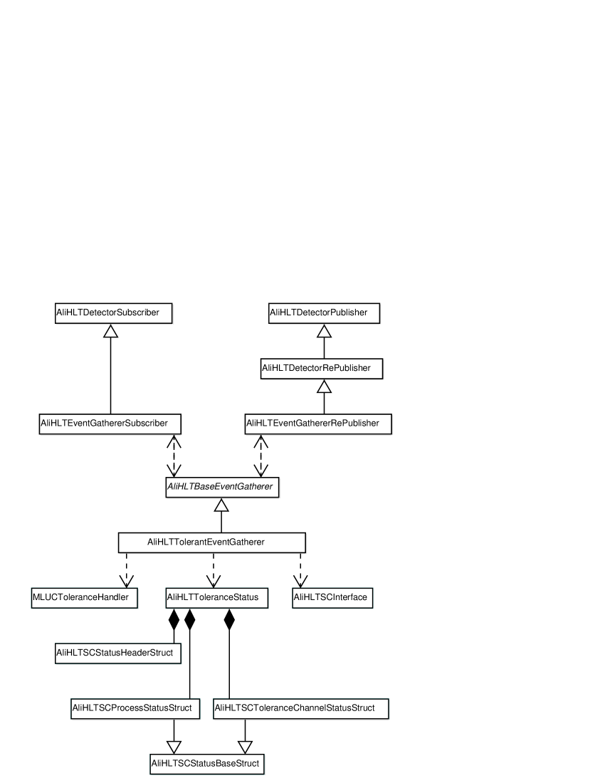
As in the case of the fault tolerant scatterer component, the fault tolerant gatherer’s main program does not differ significantly from the original gatherer one’s. The main differences are also the initialization of the added classes, primarily status structures and instances of the control and monitoring classes described in section 7.5.2.
The Fault Tolerant Event Gatherer Class
Identical to the AliHLTEventGatherer class, the AliHLTTolerantEventGatherer class is also derived from the AliHLTBaseEventGatherer class and implements its five abstract defined functions. Compared to the standard gatherer class it uses a number of additional objects or object pointers. One of these is an MLUCFaultToleranceHandler object, as described in section 4.2.1. Unlike the scatterer, the fault tolerant gatherer does not use this object to determine where to send an event or event done data, but only to keep track of the states of the paths associated with its input subscribers. To select an output path for an event done data structure, it uses the information from which subscriber the respective event has been received.
The class’s primary data structures are event lists, one for active events that have been received and announced but not yet released and a backlog list holding a configurable amount of event done data structures for already released events. In the first list EventGathererData structures are stored, similar to the original gatherer class’s event data list. Included in this data structure is a pointer for each event to the subscriber object from which it has been received and the index number associated with that subscriber. Events are added to the active event list in the NewEvent function when a new event is received and in the EventDone function when an error occurs sending the event done data back to an event’s original publisher. Additionally, events are added to the backlog list in the EventDone function after their event done data structure has been sent successfully to its originating publisher.
Fault tolerance functionality provided by the class is primarily located in three of its functions: NewEvent, EventDone, and SetSubscriber. NewEvent is called by one of the component’s subscriber objects when a new event has been received and EventDone is called by the republisher after an event has been released. SetSubscriber is called by the ProcessCmd function upon receipt of a command indicating that the state of one of the input paths has changed.
When the NewEvent function is called with a new event by one of the component’s subscribers, the list of active events is first searched whether the event has been received already. If the event is found in that list, the subscriber pointer and index in its data structure are changed to the corresponding ones of the subscriber from which it has just been received again. When a flag is set in the event’s data structure to signal that the event has been released already, the respective event done data that has been received will be sent back to the subscriber from which the event has just been received. This is done immediately without announcing the event again through the component’s output publisher.
If the event is not contained in the active event list, the backlog list is searched as well and when the event is found in that list, its event done data contained in the list is sent back immediately as well. Events not contained in either list have been received for the first time or have already been removed from the backlog list. This last case should not happen if the backlog list is large enough. An EventGathererData structure for the event is created, filled, and added to the active event list. The pointer to that data is added to the signal object used to notify the component’s main loop about new events. After adding the event’s data to the signal object it is triggered to wake up the main loop and initiate the republishing of the event.
In the class’s EventDone function, called when an event has been released, the data structure for it is searched in the list of active events first. Once its data has been found, the pointer to its subscriber and the subscriber’s index number are extracted. The subscriber index is used together with the fault tolerance handler object to determine whether the subscriber and its associated path are in a working state. If this is the case, then the received event done data is passed to the subscriber’s EventDone function to signal the event’s original publisher that it can be freed. Following the successful completion of this, the event’s data is removed from the list and any resources occupied by its data are released. Finally, the event done data is added to the end of the backlog list of released events. That list’s first element is then removed if it has become too long. When an error has occured in EventDone, the data structure remains in the list of active events. For an event whose subscriber is marked as faulty in the fault tolerance handler object, a flag is set in the event’s data to indicate that it is already released and the received done data is stored in its data structure as well. In this case neither of the two lists is modified. When the event is subsequently received again through a different subscriber, it is not forwarded through the republisher again, but the event done data is immediately sent back, as written in the description of the NewEvent function.
The last of the important fault tolerance related functions is the SetSubscriber function, called when a command is received to change a subscriber’s and its associated path’s state. Unlike the TolerantEventScatterer’s function of the analogue name, this function does not contain much functionality. It searches for the subscriber specified in its arguments to determine its index. Using the index it sets the state of that subscriber in the fault tolerance handler object to the one specified. As the events concerned will be resent through other paths by the event scatterer, they will be received again through different subscribers as well. When an event is received again, it can be released using the new subscriber, thus no further action is necessary in this function.
A fourth, additional, function that performs a task related to the fault tolerance is the SubscriberError function. This function is called for a subscriber object when an error occurs while sending an event done message back to that specific subscriber’s publisher in EventDone. The function determines the subscriber’s index number and then sets the subscriber’s state to faulty in the component’s status data structure. To inform a supervising instance of this change it triggers a LookAtMe interrupt for all specified supervisor components, which will later cause the corresponding path to become disabled.
7.5.8 Fault Tolerant Bridge Components
The last fault tolerance components are the TolerantSubscriberBridgeHead and the TolerantPublisherBridgeHead, extensions of the SubscriberBridgeHead and PublisherBridgeHead components from section 7.1.4 respectively. Unlike the fault tolerant scatterer and gatherer components they do not replace their central AliHLTSubscriberBridgeHead and AliHLTPublisherBridgeHead classes. Instead the necessary functionality is contained in additional classes used in these components. Parts of the functionality of the two bridge head classes have not been covered in the classes’ sections in 7.1.4 as they are used in conjunction with the control and monitoring classes from 7.5.2. These parts of the classes are explained in the following paragraphs. Differences between each component and its respective basic counterpart are principally identical in the two bridge head types with only minor deviations. As this section focuses on the differences between the basic and fault tolerance components, both bridge head types are described together with comments on their respective deviations.
Compared to the basic bridge components the major additional tasks in the two components’ main programs are the parsing of command line parameters for the fault tolerant relevant configuration as well as the creation, configuration, and activation of required additional objects. In addition to the objects of the classes described below, this includes primarily an instance of the AliHLTSCInterface class, described in section 7.5.2, to allow the external control of the components.
Additional Bridge Head Class Functionality
The ability to change remote message and blob-message addresses during runtime of the component is a feature contained in both bridge head classes. To ensure that this does not happen at times when the communication classes or addresses are in use, locks have been introduced in the classes to protect the regions in the class methods where they are used. These locks have to be acquired by an external entity before it attempts to modify the remote addresses of a bridge head object. An additional feature that should also be used before changing addresses, is the ability to pause processing in the classes. If a bridge head object is paused, no events are processed, new events are not announced to the publisher bridge head component, and neither are event done messages sent to the subscriber bridge head. Pausing the objects before modifying the communication addresses ensures that no communication attempt is made during the process of modification.
To support communication with the fault tolerance parts without introducing customized bridge head classes or adding optional functionality to the bridge head classes themselves, three additional classes and structures can be attached to bridge head objects. The first of these external structures is a LAM proxy object derived from a common abstract base class, AliHLTBridgeHeadLAMProxy. Its only function, LookAtMe, is called by the bridge head objects when an error occurs in their Connect function while trying to establish a connection to their remote partner. In the LAM proxy derived class used in the fault tolerant bridge components the LookAtMe function sends LAM requests to a configured list of supervisor component addresses. This address list is provided to the component via command line parameters and can contain multiple target components.
Next to the LAM proxy object an instance of the AliHLTBridgeStatusData structure is the second external object used in the bridge classes. This structure contains status data for a bridge component and consists of a header field, a generic process status field, and a bridge status field. In this last field two elements are contained, signalling the connection status of the message communication object as well as the combined connection status of the blob and blob-message objects. Both communication status fields are updated in the bridge classes’ Connect and Disconnect functions as required.
The third external entity that can be used is an error callback, derived from the AliHLTBridgeHeadErrorCallback template class. It contains two abstract functions, ConnectionError and ConnectionEstablished. The first is called when a communication error occurs, including message sends, blob transfers, or connection or disconnection attempts. In the derived class used in the bridge head components this function pauses the bridge object in the component and calls its Disconnect function to abort the connection. A later communication attempt automatically initiates a reconnection attempt of the communication objects by calling the classes’ Connect function. When this function completes successfully with a new established connection, the callback object’s second function, ConnectionEstablished, is called to signal the new connection. The fault tolerant bridge component callback object then acknowledges the connection by restarting the paused object.
In addition to the address change ability and the use of the above three external classes one more function is contained in the class used for the fault tolerance functionality, PURGEALLEVENTS. When this function is called it will access all data fields in the corresponding bridge object and remove any contained event data structures. After this function has been called, the object is in a state of not having received any event, making this function inherently dangerous since calling it can cause events to be lost in a system. This functionality is required to bring the objects into a known clean state after a connection to one remote partner has been aborted and before a new connection to another remote bridge component is established. In this situation no events will be lost as the scatterer takes care to resend them.
Fault Tolerant Bridge Command Handler
In the two fault tolerant bridge components the most important objects in addition to the three external ones attached to the bridge objects are the command processors that handle commands received from external supervisor components. The ProcessCmd functions are able to handle five commands related to the bridge’s connections: Disconnect, Connect, Reconnect, NewConnection, and NewRemoteAddress. For the first two just the bridge objects’ Disconnect and Connect functions are called respectively. A Reconnect command causes Disconnect and Connect calls in succession, with the bridge object being paused before and restarted after the calls. For the Reconnect command the communication lock is acquired before and released after the two connection function calls, the two simple Connect and Disconnect commands do not use the locks.
The last two commands both contain new message and blob-message addresses for the remote partner bridge head of the component. It is not necessary to transmit the remote blob address as it is queried using the blob-message object. After extracting the two addresses from the command structure the bridge head object is paused, its communication lock is acquired, and a currently established connection is terminated using the Disconnect function. With the connection interrupted the new address is passed to the bridge head object, and in case of the NewConnection command, Connect is called to reestablish the connection. Following this, the communication lock is released again and the object is restarted.
In addition to the five connection-related commands, one more command is available for processing by the command handler objects. The PURGEALLEVENTS command clears all events from the bridge object by calling the object’s function of the same name described above.
Chapter 8 Benchmarks and System Tests
Results of tests executed with the developed software are presented in this section. First short micro benchmarks are presented, followed by network reference tests. These reference tests are used for comparison and evaluation of the subsequent benchmarks of the two TCP communication classes. In the next section benchmarks and scalability evaluations of the basic publisher-subscriber interface are presented. The final section contains descriptions and results of two tests of the complete framework: A performance test using simulated ALICE TPC data with ALICE analysis components and a test of the framework’s fault tolerance functionality. The operating system used in all tests except for the logging overhead measurement (section 8.1.1) was a SuSE Linux [133] [134] version 7.2 running a Linux kernel version 2.4.18 [135] with the precise accounting [141] (cf. section 8.2 below) and bigphysarea patches [118] applied. For the logging overhead measurement a standard SuSE Linux 8.0 was used. The corresponding data can be found in appendix B.
8.1 Micro-Benchmarks
8.1.1 Logging Overhead
The logging system available in the MLUC class library was designed so that logging calls for messages with deactivated severity levels impose as little overhead for the calling program as possible (see also section 4.2.1). For calling the logging system with multiple severity levels two major variants are possible. The first is a function call using all required parameters. Whether a specified message has to be logged is decided inside the function based upon its severity and the activated severity levels. The other variant for calling the system is by using an if-statement to decide whether logging takes place followed by a function call to execute the actual logging process in the case of a positive decision.
To evaluate the effects of these two variants, a small program has been written to determine the amounts of time required to execute an if-statement and a function call. The program itself is listed in appendix A.1.1. Results obtained from the program are shown in Table 8.1 without compiler optimization and Table 8.2 with compiler optimization level 2 (-O2) for a gcc 2.95.3 compiler for an i686 (-march=i686) processor. Execution of the program was performed on a 700 MHz Pentium III processor. Absolute execution times, though, are not as important as the values relative to each other. The first column of each table, labeled Reference Loop, includes only the time for a loop with just one pointer dereference increment (*n++). This pointer dereference increment is used as the test instruction for the if-statement tests and the function calls. It is included in the reference loop to prevent the compiler from removing it during optimization and is therefore also kept in each examined statement for comparison. Each of the different loop tests is executed times to obtain good accuracy. In addition each test has been run ten times with the values shown averaged over these ten runs. For the exact instructions executed in each case see appendix section A.1.1.
| Measurement | Reference Loop | Loop w. if | Loop w. | Loop w. if | Loop w. func. |
|---|---|---|---|---|---|
| function | & func. | cont. if | |||
| Time per loop iteration / | |||||
| Time per loop iteration w/o | - | ||||
| overhead / |
| Measurement | Reference Loop | Loop w. if | Loop w. | Loop w. if | Loop w. func. |
|---|---|---|---|---|---|
| function | & func. | cont. if | |||
| Time per loop iteration / | |||||
| Time per loop iteration w/o | - | ||||
| overhead / |
Taking into account the reference loop overhead one can compare the time required for a loop using an if-statement with the time for a loop using a function call and an if-statement. As a result of these comparisons one can conclude that a function call containing an if-statement, corresponding to the first logging call option, is 8 to 14 times slower than just an if-statement, corresponding to the second option. The efforts in making the logging system handle calls with disabled levels efficiently are thus justified. Even with activated logging, corresponding to the case for an if-statement followed by a function call, the approach chosen is more efficient than a function call containing an if-statement.
8.1.2 Cache and Memory Reference Tests
In addition to the framework tests, three reference PCs, described below, have been examined with a cache testing program [136] to obtain the different amounts of time required to access data stored in the level 1 cache, level 2 cache, and main memory respectively. These times are necessary for the evaluation of the scaling behaviour of the programs tested. They are measured by accessing memory arrays of varying sizes with different distances between the array fields (strides) accessed. From the graphs obtained by plotting the access times in dependance of array size and stride one can determine, amongst others, the different access times. Figures 8.1, 8.2, and 8.3 contain the three different plots that have been obtained by running this program on the reference PCs. Table 8.3 summarizes the values for the different access times. During the tests the number of background processes, e.g. system daemons, has been restricted to a minimum to exclude outside interference effects as far as possible. The list of remaining processes is shown in appendix A.2. For similar reasons any networks in the machine have been disabled and unplugged for the duration of the tests.
All of the three reference PCs listed below have dual Pentium III processors with a 133 MHz front side bus using PC133 SDRAM memory in a two bus interleaved mode, doubling the theoretical memory bandwidth.
-
•
733 MHz PC with the Katmai P3 version with 16 kB Level 1 data cache and 256 kB unified Level 2 cache running at half the CPU’s clock frequency. This PC uses a Tyan Thunder 2500 motherboard with the Serverworks III HE chipset.
-
•
800 MHz PC with the Coppermine P3 version with 16 kB Level 1 data cache and 256 kB unified Level 2 cache running at full CPU clock frequency. This PC uses a Tyan Thunder HEsl motherboard with the Serverworks III HEsl chipset, the successor to the III HE chipset.
-
•
933 MHz PC with the Coppermine P3 version with 16 kB Level 1 data cache and 256 kB unified Level 2 cache running at full CPU clock frequency. This PC uses a Tyan Thunder HEsl motherboard with the Serverworks III HEsl chipset, similar to the motherboard in the 800 MHz PC.
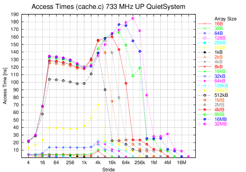
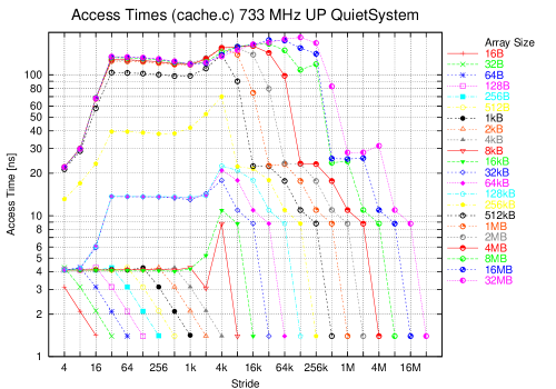
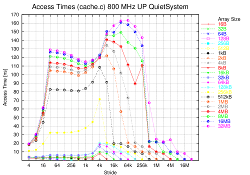
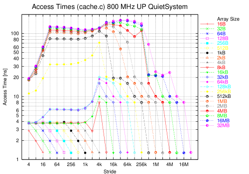
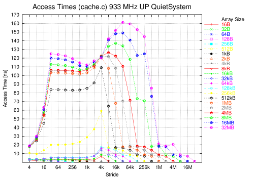
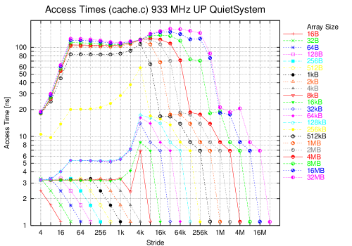
| 733 MHz PC | 800 MHz PC | 933 MHz PC | |
|---|---|---|---|
| Level 1 Cache access time / ns | 4.1 | 3.8 | 3.2 |
| Level 2 Cache access time / ns | 13.6 0.06 | 6.2 0.06 | 5.3 0.06 |
| Memory access time / ns | 127 8 | 114 14 | 113 12 |
All cache measurements have been executed with the operating system running in single CPU mode, as exchanging the processes between the two CPUs would influence and distort the results. The effects of the three different types of PCs can clearly be seen in the measured access times shown in Table 8.3. The level 1 cache access times scale very well with the CPUs’ clock frequencies. Level 2 cache times also show good scaling with the respective level 2 clock frequencies, taking into account the factor of 2 in the 733 MHz PC. Memory access times are primarily influenced by the chipsets as the access times on the two similar motherboards are basically identical, irrespective of the CPU clock frequencies. These measured times will be used later in the scaling evaluations of the publisher-subscriber communication properties.
One results of the cache and memory benchmarks is not fully understood so far. This is the linear behaviour of the last four points of each curve between 16 B and 4 kB array sizes, with decreasing times for larger strides. These behaviours can best be observed in the logarithmic plots for each reference PC. Due to the displayed behaviour cache properties (e.g. cache size, cache line size, or associativity) are unlikely to be the causes for this phenomenon. Possible explanations include pipelining or queueing effects in the processor, e.g. branch prediction or data forwarding effects. However, an exact explanation would require a very intimate and detailed knowledge of the internal processor architecture, which could not be obtained as part of this thesis. A qualitatively similar behaviour can be observed on a HP V-Class machine, while differing effects in this array size range can be observed on an AMD Athlon, a Pentium 4, and a SUN Enterprise 10000. For the measurements the plateau results before the decrease have been used. The actual value displayed on the plateau corresponds very well to the documented [137] 3 cycle load latency for a L1 cache hit of the Intel PentiumPro system architecture on which the Pentium III is based [138].
8.2 CPU Usage Measurements
For several measurements in this chapter CPU loads on PCs running Linux had to be measured. During some of these tests strange behaviours could be observed which could be traced after some careful examination to the method of timeslice (and thus CPU usage) accounting in the Linux kernel [139], [140]. These values are exported by the kernel via its /proc interface and are used as the basis for all CPU accounting and usage programs, e.g. top or xosview as well as the MLUC monitoring classes in section 4.2.1. As part of [139] a Linux kernel precise accounting patch [141] has been written which allows a global as well as process CPU usage accounting using the time stamp counter of the processor. Using this patch CPU usage accounting can thus be done on the granularity of the CPU’s clock frequency, much more accurate than the default kernel accounting based on a 10 ms timeslice granularity. This patch has been used to determine the CPU load in all measurements in this chapter.
8.3 Network Reference Tests
To determine the influence of the network hardware and the operating system on the TCP communication class benchmarks, a number of measurements have been performed using a C program that directly accesses the socket API to perform TCP communication. The tests have been executed four times, for Fast and Gigabit Ethernet with and without the TCP_NODELAY socket option set respectively. For each of these four test types the message sending latency as well as the throughput in the mode of a continuous stream of packets to a receiver have been measured. In a preparatory measurement the number of blocks has been determined which is to be sent in a stream for each block size in the throughput tests. This block count has been determined by sending varying numbers of 32 byte large blocks in a continuous stream to a receiver and plotting the achieved sending rate for each block count.
The tests have been performed on four pairs of the 800 MHz reference PCs examined in section 8.1.2, using the PC’s onboard Intel EEPro 100 Fast Ethernet interfaces as well as 3Com 3C996T Gigabit Ethernet adapter cards (based on a Broadcom chip) in 64 bit/66 MHz PCI slots on the boards. As the maximum transmission unit (MTU) 1500 B has been specified for both interfaces. For the Fast Ethernet interfaces the standard kernel drivers were used while for Gigabit Ethernet a driver supplied by Broadcom [142], [143] was used in version 2.2.19. For each measuring point 10 measurements have been made with the average used as the result for that point.
8.3.1 TCP Network Reference Throughput
Plateau Determination
To determine the block count for the throughput measurement varying numbers of blocks of the same size have been sent in direct succession to a remote receiver. Blocks of 32 bytes are transmitted in a varying number from 1 to (8388608 / 8 M). To calculate the sending rate the time required for all blocks to be sent has been measured as the program’s main output. The expected shape of the resulting curve is a rise that flattens to slowly approach an asymptotic value. Actual obtained results are shown in Fig. 8.4. None off the four tests displays the expected behaviour. The one that most closely follows the predicted form is the Gigabit Ethernet test without the TCP_NODELAY option. Instead each test shows the same approximate form of its curve, a steep rise to a maximum value followed by a decrease that levels off to approach an asymptotic value for large message sizes. For the two tests with the TCP_NODELAY option set the decreases even reach a minimum and rise again slighty towards their asymptotic values. The respective peak and asymptotic values for the achieved sending rate are shown in Table 8.4 together with the block count for each rate’s peak value. An interesting fact observed is that both pairs of Gigabit and Fast Ethernet tests reach approximately the same asymptotic value for large counts, showing no effect of the TCP_NODELAY option for large block counts. This behaviour is explained by the fact that the Linux Kernel only evaluates this option if specific preconditions are met, e.g. all large blocks queued have been actually sent. The results indicate that these preconditions are met only rarely in these tests, thereby reducing the option’s effect on the measurements.
One immediate fact that can be derived from this measurement is the overhead involved in doing a write call for a 32 byte block (or message). As the overhead for writing the actual amount of data can be neglected, this approximates the minimal overhead of a write call. The overhead can be determined by taking the inverse of the measured maximum sending rate. For Gigabit Ethernet this is approximately 1.8 and for Fast Ethernet it is about 2.7 . Note that this overhead only definitely includes the TCP protocol overhead until the network packet has been generated and enqueued for transmission. The actual transmission until the packet reaches the physical network medium will mostly not be included here.
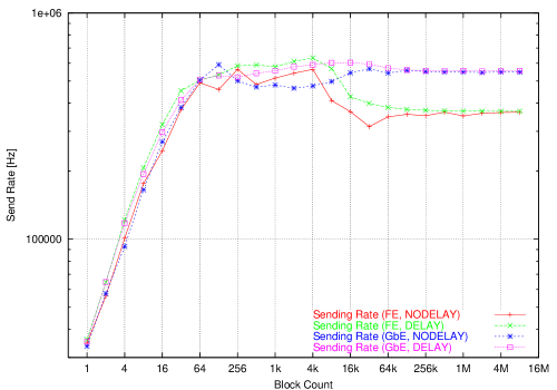
| Test Type | Peak Value / | Peak Value | Asymptotic Value / |
|---|---|---|---|
| Hz | (Block Count) | Hz | |
| Fast Ethernet | 563600 | 4096 | 364000 |
| with TCP_NODELAY | (4 k) | ||
| Fast Ethernet | 633000 | 4096 | 367800 |
| without TCP_NODELAY | (4 k) | ||
| Gigabit Ethernet | 590900 | 128 | 547000 |
| with TCP_NODELAY | |||
| Gigabit Ethernet | 603700 | 16384 | 555000 |
| without TCP_NODELAY | (16 k) |
Plateau Throughput Measurement
A message count of 524288 (512 k) blocks has been chosen for the plateau throughput measurements as all four tests have approached their asymptotic plateau value closely at this count in the prerequisite measurement. The results obtained from these tests are displayed in Fig. 8.5 to 8.9.

Fig. 8.5 displays the block sending rate achieved in the tests. As can be seen the Fast and Gigabit Ethernet test pairs are almost identical with only slight deviations at small message sizes. Starting at about 64 B for Fast Ethernet (FE) and 512 B for Gigabit Ethernet (GbE) the curves become basically linear with identical slopes. Both sets differ by about a factor of 6. The similarity of each pair can be explained by the same reasoning as for the limited effect of the TCP_NODELAY option in the first measurement in this section. In theory the difference between the two sets for Gigabit Ethernet (1 Gbps) and Fast Ethernet (100 Mbps) should be a factor of 10. The reason why this factor is only 6 is that the used GbE cards are not able to saturate the GbE link, whereas the FE cards are able to saturate their link. This is also shown in comparison with the curves showing the maximum theoretical sending rate for each of the two networks. For FE the measured sending rate approaches the theoretical limit very quickly. In contrast for GbE the limit is approached for larger blocks and the measured rate is limited by another factor, as it runs parallel to but does not approach the theoretical curve. The factor between the theoretical and the measured curves is about 1.7, indicating that the used GbE adapter cards only utilize about 60 % of the network’s theoretical bandwidth.
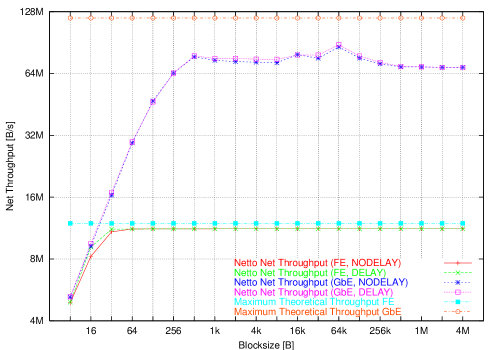
Test results obtained for the network throughput can be seen in Fig. 8.6. They have been obtained by multiplying the measured sending rate with the respective block sizes so that they reflect application level throughput that can be achieved by a program. In analogy with the rate test results, the initial rise levels off to a constant plateau at 64 B for FE and 512 B for GbE, and the same approximate factor of 6 between the two sets becomes apparent. Two effects of both Gigabit Ethernet tests could not be observed so clearly in the rate curves. The first of these are deviations between 16 kB and 64 kB blocks. In this interval they rise above the surrounding plateau level and display a peak at 64 kB blocks of around 86 MB/s. The second effect is that the network throughput actually drops slightly with increasing block sizes, going from 77 MB/s for 512 B blocks to 68 MB/s for 4 MB blocks. This seems to indicate that for Fast Ethernet the limit is set by the saturated network link, while for Gigabit some effect on the PC, e.g. from the network card, the operating system, or the PCs memory, limits the throughput. This can again be seen in comparison with the theoretically achievable throughputs. For FE one can see in this figure that in the plateau the measured throughput is about 94 % of the theoretical maximum. The missing 6 % are due to the TCP/IP protocol overhead, the protocol headers for each network packet which also require some of the available bandwidth. For GbE in contrast only between about 72 % and about 58 % of the available bandwidth are used. Accounting for the 6 % TCP protocol overhead, as determined from FE, one can see that with the GbE cards used in the test between 22 % and 36 % of the available bandwidth are not used.
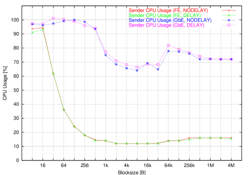
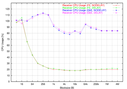
CPU usage measured during the tests is shown in Fig. 8.7, on the left hand side for the sender and on the right for the receiver. The first fact to become apparent is the identity of the sets of Fast and Gigabit Ethernet respectively, with the FE curves lying practically on top of each other. For Fast Ethernet on the sender as well as on the receiver the shape of the curve is an initial steep decrease that levels off to an almost flat plateau, with only a slight “bathtub” minimum at its center. An exception to the initial decrease are the 8 B block measurements whose results are slightly lower than the ones of the following 16 B blocks. As can be expected, absolute usage values on the receiver are slightly higher than those on the sender. Maximum values are at 102 % and 96 % for 16 B blocks on receiver and sender respectively and minimum values at 18 % between 4 kB and 32 kB and 12 % between 2 kB and 32 kB. For Gigabit Ethernet the absolute values are higher and the “bathtub” shape is more pronounced. Maximum, minimum, and final values on receiver and sender respectively are at 114 %, 78 %, and 84 % and 100 %, 64 %, and 72 % respectively. Corresponding block sizes are 256 B, 8 kB, 4 MB, 128 B, 8 kB, and 4 MB. In these GbE test results the curves on both nodes also display irregularities between 16 kB and 64 kB, with the 64 kB values being at a local maximum. One result from these tests that has to be considered is the fact that the CPU usage during the GbE test reaches values larger than 100 %. This means that a single CPU computer will be fully saturated in these parts of the test and will not be able to reach the data transfer rates displayed in Fig 8.5 and 8.6.
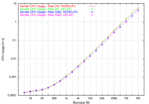
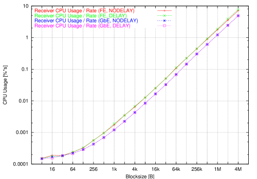
For a better comparison CPU usages of the different tests have been divided by the respective sending rates and network throughputs, with the results displayed in Fig. 8.8 and Fig. 8.9. The first of these two is a measure for the CPU overhead per send call or per message, while the second one measures the overhead per transferred byte/s. In the plots in Fig. 8.8 showing the usage relative to the sending rate no difference can be observed between the two pairs of FE and GbE curves each. In a comparison of the two different sets the Fast and Gigabit Ethernet curves are almost identical for small messages. At about 1 kB on the sender and 128 B on the receiver the curves start to diverge and the values for GbE become smaller and thus better. The difference for the largest blocks is about a factor of 1.35 on the sender and 1.45 on the receiver. One can see that the minimum CPU overhead on the sender for each message (per second) is about for the smallest messages, increasing to about and for the largest messages on Fast and Gigabit Ethernet respectively. On the receiver the values are about and for FE and and for GbE. Using the results for a specific block size it is also possible to calculate the expected CPU usage resulting from transferring blocks of that size with a given rate.
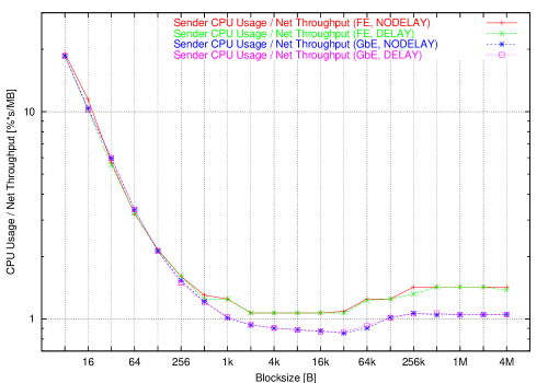
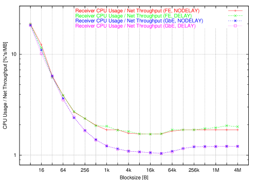
The graphs in Fig. 8.9 display CPU usage normalized with achieved throughput. They show that up to 512 B blocks on the sender and about 64 B on the receiver the four respective curves are basically identical. They start to diverge for increasing block sizes, with the Gigabit Ethernet curves at lower values than the Fast Ethernet ones. Seven of the eight curves exhibit an initial sharp decrease, that flattens to a minimum in a slight “bathtub” and then develops into a plateau. The exception is Fast Ethernet without the TCP_NODELAY option on the receiver. In this test a pronounced plateau does not set in at all, just an indication of it is showing at the last two block sizes of 2 MB and 4 MB. From these results one obvious conclusion can be drawn: Gigabit Ethernet is more efficient than Fast Ethernet concerning its use of CPU cycles per megabyte of transferred data per second. In a second conclusion one can see that, since some of the measured values are larger than , a single CPU machine will be fully busy already at values below 100 MB/s, before a GbE link will be saturated. A third result to be deduced is that it is not necessarily the most efficient approach to send at the largest possible block sizes. The minimum CPU overhead per byte transferred can be found at the medium block sizes, between about 2 kB and 32 kB on the sender and 8 kB and 32 kB on the receiver.
Peak Throughput Measurement
In addition to measuring the network transfer characteristics at the plateau values the same measurements should be performed at those block counts where the curves in Fig. 8.4 show their peak values. Unlike the throughput plateau the peak values of the four curves do not show at identical message counts. Block counts of 4 k, 4 k, 128, and 16 k therefore have been used for Fast Ethernet with and without the TCP_NODELAY option and Gigabit Ethernet with and without TCP_NODELAY respectively, as determined in section 8.3.1. Results obtained from these tests are shown in Fig. 8.10 to 8.14.
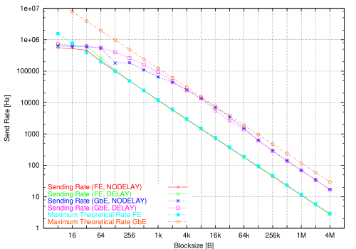
Measured rates of these tests are shown in Fig. 8.10. As can be seen, the Gigabit Ethernet rates are slightly higher than for the respective plateau test, although more deviations are present. Particularly noticeable is the drop at 128 B for the TCP_NODELAY GbE test. For Fast Ethernet only the values around 32 B for the TCP_NODELAY test and the small block measurements of the test without the TCP_NODELAY option have gained discernibly from the changed block count. Up to about 256 B the FE test using the TCP_NODELAY option is at lower values compared to the test without the option. Comparing measured and theoretical rates one can see that for GbE the theoretical limit is approached earlier and closer than in the plateau tests. For FE one can notice that for 32 B to 128 B block sizes the theoretical limit is actually exceeded by the measured curve. This result indicates that the blocks written can all be stored in local buffers, by the operating system, the network card, or both, and do not immediately reach the physical network medium. Only for larger blocks are the local buffers exceeded and the packets reach the network. This could also explain the performance increase for Gigabit Ethernet, in particular for the curve with the TCP_NODELAY option set, as this measurement uses a very small block count of only 128.
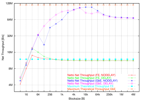
In the network throughput plots in Fig. 8.11 the differences between the plateau and peek tests are more clearly pronounced. For Fast Ethernet a peak at 32 B drops towards the same plateau as in the previous test, reached between 512 B and 1 kB large blocks. Up to about 512 B the TCP_NODELAY measurements provide values below the ones obtained without using the option. The Gigabit Ethernet curves for the TCP_NODELAY test also display the drop at 128 B. Before that drop the values are above the ones from the plateau measurement and afterwards below, up to between 1 kB and 2 kB. At larger values a local maximum is present with a peak at about 32 k, and from about 128 kB on the two test’s curves are again basically identical. For the GbE test without the TCP_NODELAY option set the values are higher than for the plateau test up to about 32 kB. Between 1 kB and 8 kB the peak results are considerably higher in the local maximum present in the peak test, the difference for the values at 8 kB is 106 MB/s compared to 75 MB/s. The comparison of the measured and theoretical curves show more clearly that the FE measurements partly exceed the theoretical limits. One can also see that the GbE curves approach their network limit much more closely than in the plateau test. This behaviour though may be just a measuring artifact, similar to the detailed FE “superperformance”.
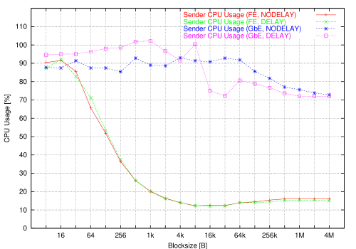
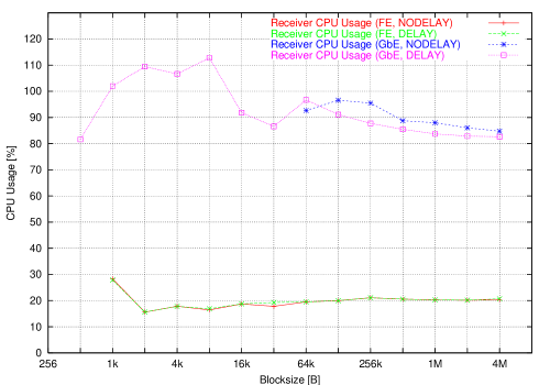
CPU usage for the sender and receiver is shown in Fig. 8.12. On the receiver the measured values for small blocks are not shown because of large inaccuracies in the respective measurements. These inaccuracies are caused by the method of measuring the usage combined with the short running times of the tests due to the small block counts. For FE the limit seems to be between 1 kB and 2 kB, while for GbE measurements up to 32 kB appear to be unreliable. At larger block sizes both FE and GbE values are basically identical to the ones from the plateau tests (Fig. 8.7). On the sending node the drop of the Fast Ethernet curves is less steep so that for block sizes below 8 kB the usage is higher than for the corresponding plateau tests. GbE results on the sender are fairly irregular and depending on the block size can be higher or lower compared to the corresponding results from the plateau measurements. Neither curve displays the “bathtub” shape as clearly as in the plateau test curves.
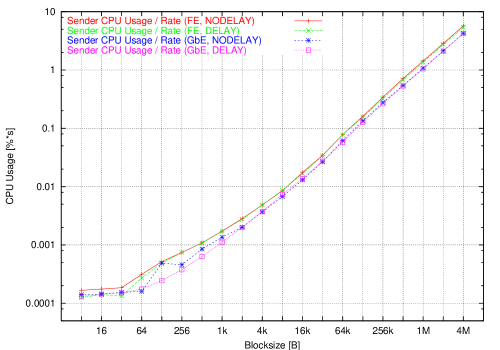
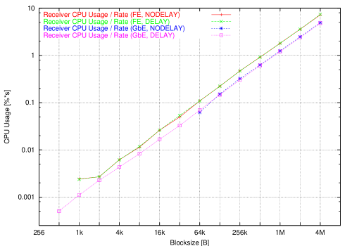
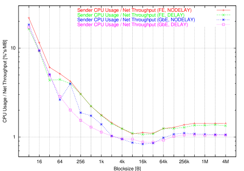
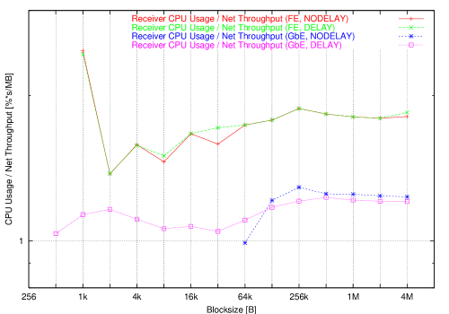
In the plots of CPU usage normalized to the sending rate and network throughput, respectively in Fig. 8.13 and 8.14, the results of the CPU usage test are reflected partially. On the receiver the measurements up to block sizes of about 2 kB for FE and 64 kB for GbE indicate unreliable values. With increasing block sizes the GbE results are approximately identical to the ones from the plateau tests, while the FE results display a slightly irregular behaviour, although at lower values than in the plateau test. The previous tests’ values are only approached for block sizes above 256 kB. On the sender the GbE curves, in particular the one from the TCP_NODELAY measurement, display erratic behaviour for small message sizes, which as on the receiver might also be caused by measurement inaccuracies. For larger blocks the curves again become basically identical to the ones from the plateau test. For FE the TCP_NODELAY curve is at higher values than its counterpart without the option up to 128 B blocks. At higher block sizes they become identical and display higher values than the respective plateau test results. Starting between 8 kB and 16 kB the FE peak test curves also become basically identical to the ones from the plateau throughput tests. Therefore, as far as the CPU efficiency is concerned, there is no significant advantage over the plateau tests, the differences on the sending and receiving nodes should approximately balance.
8.3.2 TCP Network Reference Latency
As the final network reference test the message latency has been determined by sending messages between an originating sender and a receiver. The sender transmits a number of messages to the receiver and waits for an identical reply after each message before sending the next message. By measuring the time required to send all messages and receive all replies the average message latency is determined. The results are shown in Fig. 8.15.
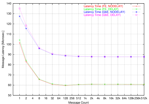
All four curves in the test display the same behaviour. With increasing message counts a drop to an asymptotically approached plateau is observed. This reflects the decrease of the relative overhead per message due to infrastructure overhead, e.g. connection establishing. The values of the two Fast Ethernet and Gigabit Ethernet test pairs are identical in the plateaus. At smaller numbers the respective results obtained without the set TCP_NODELAY option are slightly higher than the ones obtained using the option. Latency times for Fast Ethernet are consistently smaller than for Gigabit Ethernet, in the plateau the values are about compared to .
8.3.3 Network Reference Summary
As a summary Table 8.5 and 8.6 list the parameters obtained from the network reference plateau and peak throughput measurements respectively. Each entry holds the minimum and maximum values with their respective block sizes as well as the average of all values. In this table the whole range covered by the tests from 8 B to 4 MB is included. One observation can be made regarding the rule of thumb that 1 % of one CPU is used for every megabyte transferred per second. With the tested configuration this is an approximate lower bound, as almost every value of CPU usage divided by throughput is above that limit. The only exceptions are the minimal Gigabit Ethernet values on the sender.
| Rate / | Network | CPU Usage | CPU Usage | CPU Usage / | CPU Usage / | CPU Usage / | CPU Usage / | |
| Measurement | Hz | Throughput / | Sender / | Receiver / | Rate | Rate | Throughput | Throughput |
| Type | % | % | Sender / | Receiver / | Sender / | Receiver / | ||
| Reference | 2.8 @ 4 M | 4.9 @ 8 | 12 @ 2 k | 18.1 @ 16 k | 0.000146 @ 8 | 0.000152 @ 8 | 1.07 @ 16 k | 1.616 @ 16 k |
| FE w. | 643000 @ 8 | 11.2 @ 4 M | 94.4 @ 16 | 102.4 @ 16 | 5.7 @ 4 M | 7.14 @ 4 M | 19.1 @ 8 | 19.9 @ 8 |
| TCP_NODELAY | 95300 | 10.7 | 26.2 | 32 | 0.568 | 0.712 | 3.04 | 3.58 |
| Reference | 2.8 @ 4 M | 4.93 @ 8 | 12 @ 2 k | 18.1 @ 16 k | 0.00014 @ 8 | 0.000152 @ 8 | 1.07 @ 32 k | 1.616 @ 16 k |
| FE w/o | 647000 @ 8 | 11.2 @ 2 M | 93.2 @ 16 | 105.6 @ 16 | 5.52 @ 4 M | 7.66 @ 4 M | 18.44 @ 8 | 19.86 @ 8 |
| TCP_NODELAY | 99000 | 10.8 | 26 | 32.6 | 0.558 | 0.764 | 1.46 | 3.58 |
| Reference | 17.1 @ 4 M | 5.22 @ 8 | 64 @ 8 k | 78 @ 8 k | 0.000142 @ 8 | 0.000148 @ 8 | 0.854 @ 32 k | 1.044 @ 32 k |
| GbE w. | 684000 @ 8 | 86.2 @ 64 k | 100 @ 128 | 113.4 @ 256 | 4.2 @ 4 M | 4.9 @ 4 M | 18.58 @ 8 | 19.34 @ 8 |
| TCP_NODELAY | 163000 | 60.2 | 80.4 | 92.4 | 0.418 | 0.488 | 2.8 | 3.04 |
| Reference | 17.1 @ 4 M | 5.24 @ 8 | 66.4 @ 8 k | 80.8 @ 8 k | 0.000142 @ 8 | 0.000148 @ 8 | 0.866 @ 32 k | 1.038 @ 32 k |
| GbE w/o | 687000 @ 8 | 88.4 @ 64 k | 101.2 @ 32 | 112.6 @ 256 | 4.2 @ 4 M | 4.9 @ 4 M | 18.54 @ 8 | 19.38 @ 8 |
| TCP_NODELAY | 166000 | 61.2 | 81.6 | 92.8 | 0.42 | 0.488 | 2.78 | 2.98 |
| Rate / | Network | CPU Usage | CPU Usage | CPU Usage / | CPU Usage / | CPU Usage / | CPU Usage / | |
| Measurement | Hz | Throughput / | Sender / | Receiver / | Rate | Rate | Throughput | Throughput |
| Type | % | % | Sender / | Receiver / | Sender / | Receiver / | ||
| Reference | 2.8 @ 4 M | 4.13 @ 8 | 12.2 @ 8 k | 15.6 @ 2 k | 0.000166 @ 8 | 0.00242 @ 1 k | 1.084 @ 8 k | 1.38 @ 2 k |
| FE w. | 542000 @ 8 | 14.1 @ 32 | 91.6 @ 16 | 28.4 @ 1 k | 5.72 @ 4 M | 7.24 @ 4 M | 21.8 @ 8 | 2.48 @ 1 k |
| TCP_NODELAY | 96500 | 11.1 | 32.2 | 19.7 | 0.568 | 1.11 | 3.58 | 1.75 |
| Reference | 2.8 @ 4 M | 5.31 @ 8 | 12 @ 16 k | 15.6 @ 2 k | 0.000126 @ 8 | 0.00238 @ 1 k | 1.068 @ 16 k | 1.38 @ 2 k |
| FE w/o | 696000 @ 8 | 19 @ 32 | 92.2 @ 16 | 27.8 @ 1 k | 5.36 @ 4 M | 7.38 @ 4 M | 16.42 @ 8 | 2.44 @ 1 k |
| TCP_NODELAY | 122000 | 11.7 | 32 | 19.9 | 0.538 | 1.12 | 3.02 | 1.77 |
| Reference | 17.2 @ 4 M | 4.78 @ 8 | 72.8 @ 4 M | 84.8 @ 4 M | 0.00014 @ 8 | 0.0619 @ 64 k | 0.834 @ 16 k | 0.991 @ 64 k |
| GbE w. | 627000 @ 8 | 109 @ 16 k | 93 @ 4 k | 96.6 @ 128 k | 4.24 @ 4 M | 4.94 @ 4 M | 18.36 | 1.29 @ 256 k |
| TCP_NODELAY | 151000 | 70.8 | 86.2 | 90.3 | 0.426 | 1.4 | 2.82 | 1.21 |
| Reference | 17.1 @ 4 M | 5.52 @ 8 | 72 @ 1 M | 81.6 @ 512 | 0.00013 @ 8 | 0.000506 @ 512 | 0.872 @ 32 k | 1.04 @ 512 |
| GbE w/o | 723000 @ 8 | 106 @ 8 k | 102.2 @ 1 k | 113 @ 8 k | 4.2 @ 4 M | 4.83 @ 4 M | 17.14 @ 8 | 1.23 @ 512 k |
| TCP_NODELAY | 179000 | 66.4 | 87.2 | 92.9 | 0.42 | 0.69 | 2.6 | 1.14 |
8.4 Communication Class Benchmarks
For the communication classes benchmarks have been carried out with the TCP message and blob class implementations. The SCI classes have not been tested due to the prototype status of the implementation. Two different measurements have been executed for the message classes, measuring the message latency as well as the achievable continuous throughput during message sending as a function of the message size. For the blob classes these two tests have been performed twice, using the standard on-demand type allocation where a block is remotely allocated for each transfer as well as the preallocation method where the whole remote buffer is allocated before any transfer, and buffer management is executed locally in the sender. The hardware and system software used for the tests is identical to that used in the network reference tests, described in section 8.3. For both network adapters sending has been performed twice, with and without explicit connect calls, to determine the influence of establishing implicit connections on the transfers. Again the results of the measuring points have been obtained as the average of ten measurements each. Each test’s result is described first in detail, and then two summaries for the message and communication classes are given as well as an overall summary for the TCP communication class implementations.
8.4.1 TCP Message Class Throughput
In order to benchmark the TCP message class, measurements have been made to determine the maximum rate achievable by streaming a continuous sequence of messages to a target without waiting for a reply. This test is relevant for the comunication classes’ use in the framework which has been designed to not require a reply from a remote side anywhere. As for the network reference tests a prior measurement is used to determine the number of messages to be sent for each size by measuring the sending rate for different numbers of messages streamed to the receiver.
Plateau Determination
To determine the number of messages to be used for the following throughput measurements, a prerequisite measurement has been made for each of the four test types (FE, GbE, explicit or implicit connects (cf. sections 5.2.1 and 5.4.2)) in order to establish the influence of this number on the throughput. For the test the smallest message of 32 bytes is transmitted in a varying number from 1 to . A plateau with an asymptotic value was expected. The throughput tests were then to be performed using a message count on the plateau. To restrict the running times of the tests, the start of the plateau was intended to be used.
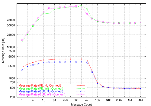
The actual results of these tests are shown in Fig. 8.16. Connected as well as unconnected tests display increasing curves to a first plateau followed by a steeper decrease to a second plateau. Peak values for all curves are reached at about 2048 (2 k) messages while asymptotic values are reached at 262144 (256 k) messages. These values are therefore used as the counts for two separate throughput measurements. The exact reason for the observed sudden decrease has not been determined yet. A possible explanation are overflows of system or network interface buffers, e.g. socket send or receive buffers, causing packet loss and retransmits, but this hypothesis has not been verified yet. One test to determine or at least narrow the cause of this drop would be to modify the benchmark program to use different socket buffer sizes, vary these over a certain range, and observe whether the drop occurs at different message counts. A variation of the message size to determine its effect on the behaviour could also be performed in separate measurements as well as in combination with the buffer size variation. Due to the large parameter space and correspondingly large amount of measurements, and the time required for them, these investigations have not been executed as part of this thesis. For the use of the framework the observed drops do not present a problem, as the communication classes are only used with explicit connections. In this mode even the values after the drop are sufficiently high for the given requirements, as will be detailed in the following sections. However, in the long run research into the phenomenon as well as modifications of the communication classes to work around it, if possible, are certainly desirable.
Plateau Throughput Measurement
At the message count of 262144 (256 k) messages the plateau has been reached for all four sending types and the first throughput measurement has been performed using this message count. The message size varied from 32 B to 1 MB with the results obtained shown in Fig. 8.17 to 8.21.
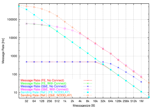
Fig. 8.17 shows the message sending rates achieved in the four tests together with the results from the reference tests. As can be seen, the message sending rate is considerably higher for the tests with explicit than with implicit connections, both for Fast and Gigabit Ethernet. This result could be expected, as in the implicit connection measurements a new connection has to be established and terminated for each message, adding the connection overhead every time. On the plateau of the two unconnected (implicitly connected) tests the rate is only limited by the overhead of establishing the connection for all messages. Only for larger messages does the rate become limited by the network limit. For the GbE test the overhead is big enough that it does not even approach the limit fully but only starts to be limited by it. In the connected test the overhead introduced by the protocol between the sender and receiver communication objects also adds overhead, decreasing the achievable message rates in comparison with the reference tests. This decrease can be primarily seen for small message sizes, for Fast Ethernet up to 256 B and for Gigabit Ethernet up to about 4 kB. For the smallest message sizes the decrease is fairly significant, a factor of 6 for FE and almost one order of magnitude for GbE. This indicates that the message class code still has some potential for optimizations. But even with these results the achieved rates in the connected mode are still easily high enough to allow the classes’ use in the framework.
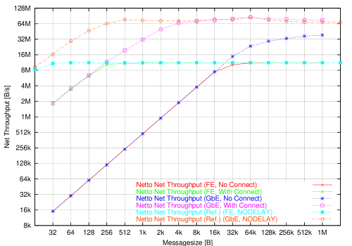
In order to show the network throughput that can be reached by an application, the achieved sending rates have been multiplied with the respective message sizes. The resulting curves are shown in Fig. 8.18. As was to be expected these curves correspond very closely to the rates from Fig. 8.17. Both Fast Ethernet as well as the connection Gigabit Ethernet curve approach the curve from their respective reference measurement, while the unconnected Gigabit Ethernet curve still rises slowly towards it. Similar to the rate curves one can see the overhead from the communication classes by the fact that they reach the hardware limit later than the corresponding reference measurement. An interesting point can be observed in the connected GbE curve. For the largest measured block sizes, from about 128 kB on, this curve even exceeds the reference curve. This behaviour indicates that the communication approach used in the class is more effective at utilizing the systems’ resources than the relatively simple reference program. Both graphs in Fig. 8.19 below support this thesis. In the receiver plot on the right hand side the receiver CPU usage of the message class is higher than the one from the reference benchmark, and in particular it is greater than 100 %, indicating that due to its multi-threaded design it is able to utilize the system’s two CPUs better. In the sender plot on the left hand side the CPU usage of the connected GbE curve is lower than the one from the GbE reference measurement for most of the test. This in turn could indicate that on the sender the communication class uses the CPU or memory system more efficiently, being therefore less constrained by it and allowing higher sending rates.
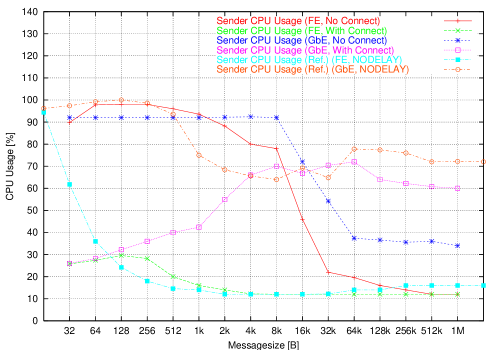
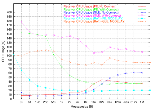
CPU usage for the sending and receiving nodes is displayed respectively on the left and right hand sides of Fig. 8.19. One obvious result that can be seen is the high CPU usage on the sending side and the very low usage on the receiver for the two unconnected measurements at small block sizes, up to about 8 kB. The reason for the very low rates at small block sizes in the unconnected mode therefore seems to be the high CPU load produced from initiating the connections on the sending node. Accepting connections on the receiving node does not seem to be so CPU intensive. A second interesting feature, as already remarked above, is the fact that on the sender the communication class CPU usage in the connected GbE test is mostly lower than the reference GbE usage. For the lower block sizes this could, in addition to the potential reasons outlined above, also be caused by the lower sending rate of the communication class in that block range. At higher block sizes, however, the throughput achieved by the communication class was higher and this reasoning cannot be applied. As outlined above at these rates it is therefore more likely that the sending approach used in the communication classes, using write preceeded by select calls, is more efficient than the simple approach of using blocking write calls in the reference benchmark program. On the receiver the behaviour of the two respective curves is reversed, the communication class consistently uses between 10 % and 20 % more CPU cycles compared to the reference benchmark. Here the communication class introduces more overhead than the reference benchmark. One likely cause of this overhead are the allocation and deallocation calls of the memory for each message as well as its copying. Similar to the reference test, the measured CPU load reaches more than 100 % and therefore uses both of the nodes’ CPUs, in particular on the receiving side. As for the reference test this implies that single CPU nodes will only be able to handle lower throughputs than measured in this benchmark.
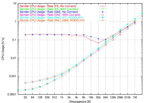
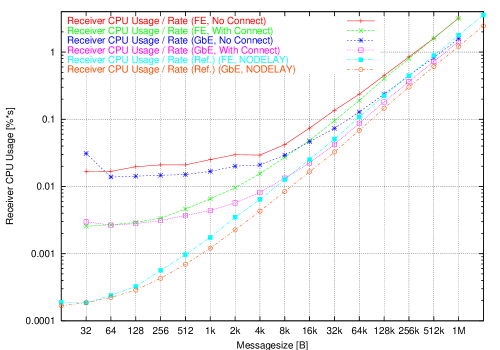
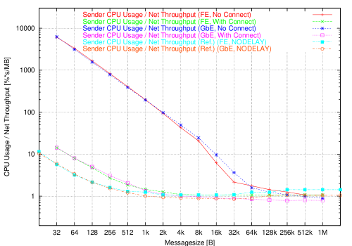
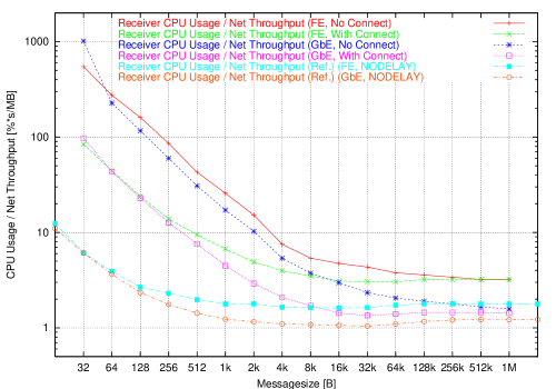
For a better comparison all CPU usage measurements should be evaluated with respect to the sending rates or network throughputs as shown in Fig. 8.20 and 8.21 respectively. The rate and bandwidth plots are correlated by the message size due to the way the network throughput is determined, as detailed above. Fig. 8.20 clearly shows the high relative overhead caused by establishing a connection for each message, particularly on the sender but on the receiver as well. This relative overhead per message can be several orders of magnitude above that for just sending a message over an established connection. In the sender graph one can also see that both connected message class measurements initially are higher than their respective reference measurement. For larger message or block sizes, however, they fall below the respective reference curve. This is a further indication for the behaviour already observed in the rate and sender side CPU usage plots (Fig. 8.17 and 8.19). In both of these single plots the message class showed better values (higher rate, smaller CPU usage) than the reference measurement for large messages. On the receiver side this behaviour is not present, here the CPU overhead outlined above is high enough that the per-message overhead of both connected message class curves is higher than the respective reference one. Similar to the reference measurement of CPU cycles per sending rate from Fig. 8.8 one can again see that Gigabit Ethernet is more efficient in its use of CPU cycles per transfer than Fast Ethernet, both on the sending and the receiving nodes. On both nodes the unconnected measurements approach the connected ones with increasing block sizes, showing that the overhead per message for establishing the connections decreases with increasing message size, as could be expected.
The plots of CPU cycles per megabyte of data transferred per second in Fig. 8.21 show mostly the same information as the ones in Fig. 8.20. One additional item can be observed in Fig. 8.21. Unlike the reference curves the connected message class measurement curves do not show a “bathtub” curve shape on the sender. At the points where the reference curves rise again the message class curves remain constant. The GbE curve even shows a slight drop. This behaviour again underlines the fact that the sending approach used in the class makes a more efficient use of CPU cycles than the one used in the reference benchmark program. On the receiver the measured message class values show the same behaviour as the reference curves, although at higher values. At small blocks the values are considerably higher, more than one magnitude for some message sizes. This shows again the high overhead added on the receiver side, presumably at least partly due to the message allocation and release calls.
Peak Throughput Measurement
At the message count of 2048 (2 k) all four sending types have reached their peak value for the measured rate. As for the plateau measurement the message size has been varied from 32 B to 1 MB with the results obtained shown in Fig. 8.22 to 8.26. Due to the short measuring times involved and the details of the measurement the CPU related values for small message sizes, particularly on the receiving node, could not be measured accurately, similar to the problems in the network reference test. These values have therefore been excluded from the measurement results.
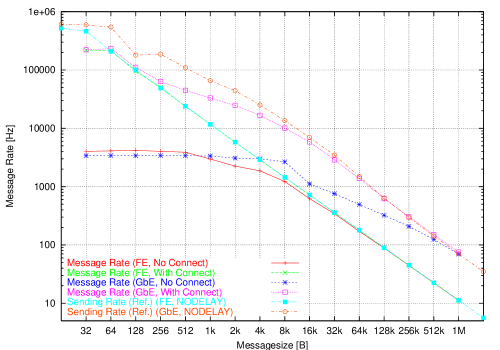
For the maximum achieved sending rate, shown in Fig. 8.22, one can see that for smaller message sizes the achieved rates are higher than for the plateau measurement in Fig. 8.17, differing by factors of about 3.6 and 8 for the connected and unconnected tests respectively. The connected Gigabit Ethernet curve runs close to the FE one up to the 256 B message size and starts to diverge for higher sizes. Both of these curves have reached their bandwidth limit at about 8 kB. For both Fast Ethernet tests as well as the connected Gigabit one the curves are identical with their corresponding plateau throughput curves for message sizes exceeding certain limits: 512 B for the connected GbE, 256 B for the connected FE, and 16 kB for the unconnected FE curve. Below that limit each peak curve features higher values than its plateau counterpart. Compared to the peak reference tests one can see that the communication class’s connected Fast Ethernet test reaches the reference sending rate earlier than in the plateau test, showing that it is less constrained by the limit at small messages encountered in that test. In the connected Gigabit Ethernet measurement the communication class reaches the respective reference limit later than the FE and later than its plateau counterpart. At about 256 B to 512 B it reaches the same values as the connected plateau GbE curve, and therefore already at these sizes seems to be limited by the same factor as the plateau measurement. The two unconnected curves initially again run almost constant, but at higher values than in the plateau test and they start to decrease earlier. At small messages the limits between these two tests thus seem to be different while the limit that causes the later decrease, most likely the available bandwidth, is approached sooner.
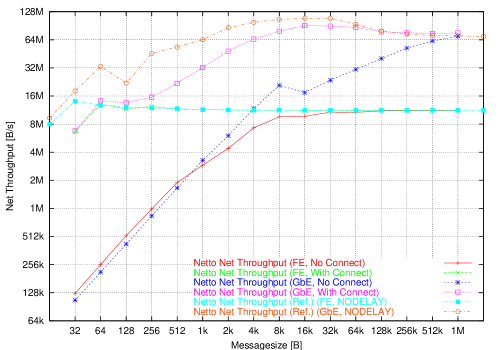
Fig. 8.23 shows the application level network throughput that has been achieved in these four tests. The respective plateau results are represented in Fig. 8.18. In consistency with the achieved rates one can see that the maximum network throughput is reached in the connected FE test for 64 B messages already. It is closely approached by the unconnected one between 8 kB and 16 kB. In both cases this happens for smaller message sizes than for the related plateau test. All four tests also start at higher throughput values and correspondingly reach the bandwidth limit earlier. The connected GbE curve is identical to the plateau curve for messages of at least 1 kB with the exception of the somewhat higher peak shifted towards the lower range between 16 kB to 32 kB. Apart from this peak the maximum values are not higher than the ones from the plateau tests, as expected. Similar to the FE reference peak measurement the message class curve reaches more than the theoretically possible network throughput. It must therefore be assumed that the data is buffered to a large degree as well. As detailed in the peak reference test this buffering is also a potential explanation for the performance increase in the peak tests. Further remarkable properties in this graph are the kinks in several of the curves. No clear explanation has been found for them yet, a possible explanation for at least some of them are buffer limits which are encountered. With full buffers the measurements then again display different behaviour as when all or a large amount of data can be buffered. Similar to reference peak tests the peak message class tests are mostly at higher throughput values than the respective plateau measurements. An exception are the FE curves where they have already reached the hardware limit.
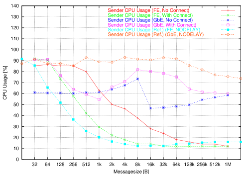
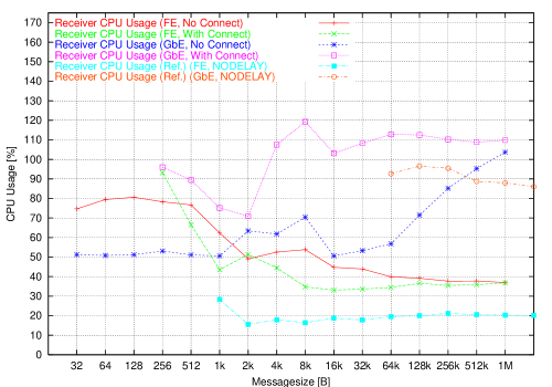
CPU usages for the tests are shown in Fig. 8.24. As for the peak reference tests some values on the receiver could not be measured accurately. These values have therefore been excluded from the graphs. As can be seen in the figures, CPU usage on the sender for the two explicit connection tests for small message sizes is much higher compared to the respective plateau test (Fig. 8.19). This continues up to the point where the usage levels become equal, for FE in the range between 32 kB to 64 kB and for GbE at about 64 kB messages sizes, similar to the observed behaviour for the sending rates and network throughputs. In the unconnected tests a different behaviour is displayed, with the FE test showing continuously lower CPU usage values coupled with an earlier decrease compared to the related plateau test. The unconnected GbE test initially displays lower values than its respective plateau throughput test, with both curves running basically flat at about 30 % and 45 % respectively. For messages sizes higher than 32 kB, though, the plateau test usage is lower. Both Fast as well as Gigabit Ethernet tests reach the same final value for the 1 MB message size. On the receiver the Gigabit Ethernet tests are mostly separated and only approach similar values for the 1 MB message size as well. The two Fast Ethernet measurements run much closer and are approximately similar. They also reach the identical values at 1 MB messages. One can also see that, similar to the plateau tests, the connected message class measurements on the sender display lower CPU usage values than the reference test; the GbE one almost over the whole test range and the FE one for large messages only. In contrast on the receiver the usage of the reference measurements, where present, is considerably lower than the message class’s, by at least 10 %. This is again similar to the behaviour in the plateau tests. On the sender the unconnected measurements are mostly at lower values than in the plateau test, while they are higher on the receiver. The difference between the unconnected usage on the two nodes is therefore not as extreme as it was in the plateau measurement where most of the load was produced on the sending node. Compared to the plateau test measurement all peak test curves can be lower or higher, depending on measurement type and message size.
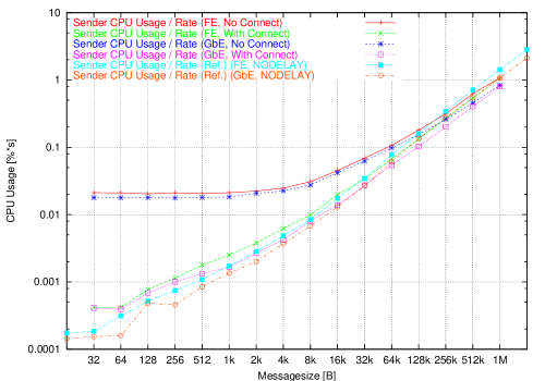
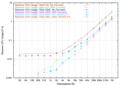
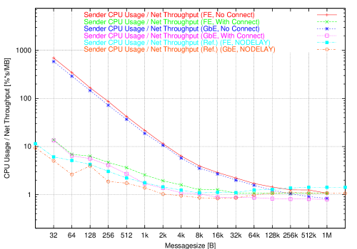
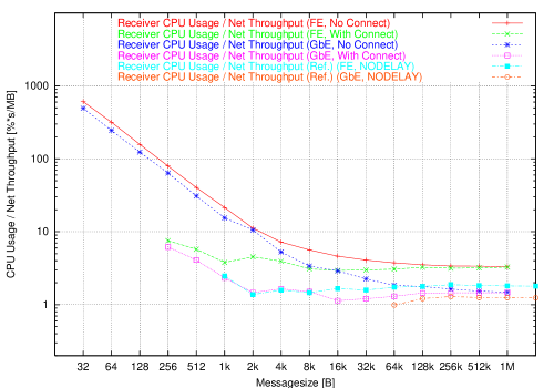
For better comparison the CPU usage values of each test are normalized to the achieved sending rate as well as to the measured network throughput, as for the plateau tests. The resulting graphs are shown in Fig. 8.25 and 8.26. For the CPU usage per rate measurements of the connected tests on the sender side one can see that the FE and GbE curves are almost identical. GbE values are slightly smaller than FE values, similar to the same measurement for the plateau tests from Fig. 8.20. Between 128 B and 2 kB inclusively the plateau curves are at lower and therefore more efficient values. From 4 kB on the curves for peak and plateau tests are almost identical, although the FE peak curve runs at slightly higher values than the plateau one. In the unconnected tests on the sender the peak test curves are a factor of about 10 lower than the plateau ones for sizes from 32 B to about 4 kB. All four curves are basically constant for this whole interval. Between 8 kB and 32 kB the peak and plateau curves show different behaviours, with the peak measurements still at lower values. From there on all four curves again show an identical linear rise. Where reliable values are available on the receiver, the four curves rise continuously with the peak curves at slightly lower values compared to the plateau ones. This trend continues up to 2 kB for FE and 32 kB for GbE, after which the respective curves in the peak and plateau tests are basically identical. For the unconnected test the corresponding peak and plateau curves appear mostly similar, although the peak curves are at slightly lower values for sizes up to about 2 kB. All four curves reach the same approximate final value for the largest messages as the respective plateau curve. In Fig. 8.25 one can see that over the whole test range each message class (and reference) GbE curve on the sender is at lower values than the corresponding FE curve. This shows that in this mode, where at least part of the data is buffered, GbE makes more efficient use of the available CPU cycles compared with FE. Also one can see again that at about 32 kB messages the connected message class measurements on the sender reach lower and better values than the corresponding reference measurement. Therefore even in this partially buffered mode the sending method in the communication class is more efficient. On the receiver the behaviour is also as before, the message class curves are higher than the reference measurements where present.
Comparing the CPU usage per network bandwidth in Fig. 8.26 and 8.21 it can be noticed that for the unconnected tests on the sender the plateau and peak test curves are almost identical in shape. However, the starting values of the two peak curves are again a factor of 10 lower than the corresponding plateau values, and only for messages greater than 64 kB do the curves show identical values. Differing from this, the peak results in the connected tests on the sending side show higher initial values. The respective curves are again almost identical after 32 kB. On the receiver node the results for the peak and plateau tests also have the same general shape, where values are available, showing a steady decrease. The peak measurements are at slightly lower values and display a slightly more unsteady behaviour. For messages exceeding 16 kB the corresponding peak and plateau test curves again run at basically identical constant values. Results obtained for the unconnected tests are almost indistinguishable in the peak and plateau tests, both in behaviour and the measured values. They show a constant decrease that flattens to constant values of about for Fast Ethernet and between and for Gigabit Ethernet. Apart from these values the same conclusions can be drawn from these graphs as already derived from Fig. 8.25.
8.4.2 TCP Message Class Latency
To determine the latency of message send operations for the different configurations a number of messages are transmitted from a sender to a receiver. For each of these messages the receiver sends a reply message to the originating sender. The sender in turn waits for this reply before sending its next message. A ping-pong message pattern is thus established between the two programs, similar to the network reference latency test principle. Results obtained from this test are shown in Fig. 8.27.
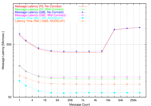
As can be seen the measured latency decreases and approaches an asymptotic plateau value for all tests, although the test remains on this plateau for the connected tests only. As expected the two unconnected tests have a latency much higher than the connected ones, due to the overhead of establishing a new connection for each new message in the unconnected (or implicitly connected) tests. The difference for the plateaus is almost a factor of 3. An unexpected and currently unexplained characteristic is displayed in both unconnected tests, starting between 8192 (8 k) and 32768 (32 k) messages, where the latency increases abruptly from about to , a factor of about 2.5. It continues to increase at a slower pace to about for 524288 (512 k) messages. The initial higher start and decrease to the plateau value is most likely explained by the measurement and infrastructure overhead that dominates the timing results obtained from the measurements so that the plateau values reflect the actual latency present in applications. An obvious exception is the unexplained rise for high message counts in the unconnected tests, which might be related to the drops shown in the graph of message rates as a function of message counts in section 8.4.1 and Fig. 8.16. But as for that graph the cause of the latency increase could not be determined in this thesis.
| Fast | Fast | Gigabit | Gigabit | Fast | Gigabit | |
| Ethernet | Ethernet | Ethernet | Ethernet | Ethernet | Ethernet | |
| Implicit | Explicit | Implicit | Explicit | Reference | Reference | |
| Connect | Connect | Connect | Connect | |||
| Average Message | 352.3 | 110.0 | 369.8 | 118.6 | 61 | 88 |
| Latency / |
Table 8.7 summarizes the minimum latency measured in each of the four tests and the reference measurements. The unconnected tests, as already detailed, are higher than the connected ones by a factor of about 3. Gigabit Ethernet tests are between 5.0 % () and 7.8 % () slower than Fast Ethernet ones for the unconnected and connected cases respectively. One can see that the differences between the respective Fast and Gigabit Ethernet measurements are, to a first order, constant. The differences between a message class measurement and the corresponding reference measurement can therefore be most probably attributed to overhead introduced in the class itself. This overhead therefore amounts to approximately and for explicit and implicit connection modes respectively.
8.4.3 TCP Message Benchmark Summary
One conclusion that can be drawn from these benchmarks is that the TCP message classes can be used in the data flow framework, especially in the ALICE HLT. The framework is designed so that message sending rates do not have to be higher than the actual event rate, and all event related message transmissions are performed over explicitly established connections. Therefore handling the 1 kHz maximum event rate required for the ALICE HLT presents no principal problem. Fulfilling this requirement is in particular aided by the fact that no reply messages are needed and thus no restriction on the minimum latency exists. At the expected message sizes between 64 B and 512 B the CPU usage is expected to be between about 0.5 % and 1.0 % on the sender and 1.3 % and 3.3 % on the receiver at the 1 kHz message rate required for proton-proton operation. These usage values are scaled to one 800 MHz CPU so that 100 % corresponds to one fully used CPU. For the 200 Hz rate of heavy-ion operation the CPU load is expected to be lower by the corresponding factor of 5. Message transfers are mainly dominated by the available memory bandwidth which does not increase as fast as CPU power, as described in section 2.1. CPU usage will most likely not decrease proportionally to the available CPU power in the future as a result. As shown in the two different throughput tests, the classes seem to perform better when the messages can be sent in short bursts than for a constant stream of messages to the receiver.
A further result that can be inferred from the tests is related to the use of Fast or Gigabit Ethernet for message transfers. If latency is not the deciding factor, as for the classes’ use in the framework, Gigabit Ethernet is the favored choice due to its lower CPU usage in sending the same amount of messages or data (Fig. 8.20 and 8.21), even if the network throughput of Fast Ethernet would already be sufficient to fulfill the requirements. Fast Ethernet cards should be chosen if latency is the primary concern, due to their lower latencies compared with Gigabit Ethernet. This of course is only possible when they are able to fulfill the bandwidth requirements. These conclusions, however, should be treated with care as they depend on the respective network adapters used and the measurements should be repeated for adapters concerned. On the other hand, due to their higher maximum throughput Gigabit Ethernet adapters are generally more efficient in their use of CPU cycles, and the technology itself sets some restrictions on the minimum latency that can be reached. Cost differences between the adapters have to be considered as well, but due to its rapid evolution this is beyond the scope of this document. As a note on the cost calculation: Using a Gigabit Ethernet card to profit from the better efficiency does not necessitate a Gigabit Ethernet switch port as well. If its bandwidth is sufficient, a Fast Ethernet switch can also be used, reducing the cost of this solution.
In a direct comparison with the network reference tests several features can be noticed, also partially reflected in the summaries of the peak and plateau throughput measurements in Table 8.8 and 8.9. A first difference can be observed in the behaviour of the sending rate in dependence of the block or message count. In the reference measurements the decrease after the initial plateau is not as obvious as in the message test. Concerning the rate and throughput it can be seen that the results from the reference measurements are much better. The plateau values differ by a factor of 9 for Fast Ethernet and a factor of 6 for Gigabit Ethernet. Differences in the peak measurements are not as large, factors of 2 and 3 can only be observed here. These comparisons only apply to the connected message tests, as expected the results of the unconnected ones are far poorer. Examining the CPU usage as well as the efficiency of CPU usage divided by throughput it can be noticed that the reference tests are better, except for the Gigabit Ethernet measurements on the sending nodes. For this case the minimum values measured are actually below the ones from the reference tests. The most likely explanation for this unexpected behaviour is that the use of write calls with timeouts followed by select calls in the message classes is more efficient for large blocks than the blocking write calls used in the reference program. Looking at the message or block latencies it is again apparent that there is a certain time penalty associated with the functionality contained in the message classes, as the results are almost a factor 2 worse for FE and 1.5 for GbE. Part of the overhead and performance decrease introduced by the message classes is certainly unavoidable due to the more elaborate checks and actions that have to be performed in them compared to the reference program. For example the reference program knows the block size in advance and can discard the data immediately after reading it. But even taking this into account, the results indicate that there still seem to be opportunities for improvement.
| Rate / | Network | CPU Usage | CPU Usage | CPU Usage / | CPU Usage / | CPU Usage / | CPU Usage / | |
| Measurement | Hz | Throughput / | Sender / | Receiver / | Rate | Rate | Throughput | Throughput |
| Type | % | % | Sender / | Receiver / | Sender / | Receiver / | ||
| Reference | 11.2 @ 1 M | 10.8 @ 32 | 12 @ 2 k | 18.1 @ 16 k | 0.000174 @ 32 | 0.000186 @ 32 | 1.07 @ 16 k | 1.62 @ 16 k |
| FE w. | 355 k @ 32 | 11.2 @ 1 M | 61.8 @ 32 | 66.2 @ 32 | 1.43 @ 1 M | 1.98 @ 1 M | 5.70 @ 32 | 6.10 @ 32 |
| TCP_NODELAY | 45200 | 11.2 | 19 | 25 | 0.175 | 0.222 | 1.71 | 2.24 |
| Reference | 11.2 @ 1 M | 11.2 @ 32 | 12 @ 2 k | 18.1 @ 16 k | 0.000168 @ 32 | 0.000180 @ 32 | 1.07 @ 32 k | 1.62 @ 16 k |
| FE w/o | 366 k @ 32 | 11.2 @ 1 M | 61.8 @ 32 | 65.8 @ 32 | 1.43 @ 1 M | 1.87 @ 1 M | 5.52 @ 32 | 5.90 @ 32 |
| TCP_NODELAY | 45800 | 11.2 | 18.9 | 25.3 | 0.173 | 0.230 | 1.69 | 2.26 |
| Reference | 68.9 @ 1 M | 16.4 @ 32 | 64 @ 8 k | 78 @ 8 k | 0.000182 @ 32 | 0.000186 @ 32 | 0.854 @ 32 k | 1.04 @ 32 k |
| GbE w. | 537 k @ 32 | 86.2 @ 64 k | 100 @ 128 | 113.4 @ 256 | 1.04 @ 1 M | 1.22 @ 1 M | 5.94 @ 32 | 6.10 @ 32 |
| TCP_NODELAY | 124 k | 65.8 | 79.5 | 92.2 | 0.130 | 0.151 | 1.55 | 1.74 |
| Reference | 69 @ 1 M | 16.9 @ 32 | 66.4 @ 8 k | 80.8 @ 8 k | 0.000182 @ 32 | 0.000182 @ 32 | 0.866 @ 32 k | 1.04 @ 32 k |
| GbE w/o | 553 k @ 32 | 88.4 @ 64 k | 101.2 @ 32 | 112.6 @ 256 | 1.04 @ 1 M | 1.22 @ 1 M | 6.00 @ 32 | 6.00 @ 32 |
| TCP_NODELAY | 125 | 67 | 80.9 | 93.2 | 0.130 | 0.150 | 1.55 | 1.73 |
| Msg Class | 11.2 @ 1 M | 1.82 @ 32 | 12 @ 8 k | 34.1 @ 64 k | 0.000434 @ 32 | 0.00256 @ 32 | 1.07 @ 1 M | 3.04 @ 64 k |
| FE | 59500 @ 32 | 11.2 @ 1 M | 29.6 @ 128 | 153 @ 32 | 1.07 @ 1 M | 3.20 @ 1 M | 14.2 @ 32 | 84 @ 32 |
| w. Connect | 15900 | 9.73 | 16.8 | 72.4 | 0.134 | 0.402 | 2.74 | 13.5 |
| Msg Class | 11.2 @ 1 M | 0.0147 @ 32 | 12 @ 512 k | 8.07 @ 64 | 0.0674 @ 32 k | 0.0167 @ 32 | 1.07 @ 1 M | 3.22 @ 1 M |
| FE | 483 @ 128 | 11.2 @ 1 M | 98 @ 128 | 44.2 @ 32 k | 1.07 @ 1 M | 3.22 @ 1 M | 6100 @ 32 | 548 @ 32 |
| w/o Connect | 343 | 5.07 | 60.1 | 23.6 | 0.254 | 0.424 | 794 | 74.6 |
| Msg Class | 75.8 @ 1 M | 1.82 @ 32 | 26 @ 32 | 106.4 @ 16 k | 0.000438 @ 32 | 0.00266 @ 64 | 0.788 @ 256 k | 1.35 @ 32 k |
| GbE | 59500 @ 32 | 85.3 @ 64 k | 72 @ 64 k | 177 @ 32 | 0.792 @ 1 M | 1.43 @ 1 M | 14.3 @ 32 | 97.6 @ 32 |
| w. Connect | 21900 | 50.7 | 53.3 | 131.4 | 0.100 | 0.181 | 2.66 | 12.8 |
| Msg Class | 38.5 @ 1 M | 0.0147 @ 32 | 34 @ 1 M | 6.66 @ 64 | 0.0994 @ 64 k | 0.0138 @ 64 | 0.882 @ 1 M | 1.58 @ 1 M |
| GbE | 483 @ 2 k | 38.5 @ 1 M | 92.4 @ 4 k | 61 @ 512 k | 0.882 @ 1 M | 1.58 @ 1 M | 6240 @ 32 | 1020 @ 32 |
| w/o Connect | 384 | 11.9 | 70.9 | 26.6 | 0.242 | 0.220 | 780 | 93.8 |
| Rate / | Network | CPU Usage | CPU Usage | CPU Usage / | CPU Usage / | CPU Usage / | CPU Usage / | |
| Measurement | Hz | Throughput / | Sender / | Receiver / | Rate | Rate | Throughput | Throughput |
| Type | % | % | Sender / | Receiver / | Sender / | Receiver / | ||
| Reference | 11.2 @ 1 M | 11.2 @ 256 k | 12.2 @ 8 k | 15.6 @ 2 k | 0.000186 @ 32 | 0.00242 @ 1 k | 1.08 @ 8 k | 1.38 @ 2 k |
| FE w. | 462 k @ 32 | 14.1 @ 32 | 85.6 @ 32 | 28.3 @ 1 k | 1.43 @ 1 M | 1.81 @ 1 M | 6.08 @ 32 | 2.48 @ 1 k |
| TCP_NODELAY | 54200 | 11.7 | 26.8 | 19.6 | 0.175 | 0.329 | 2.2 | 1.74 |
| Reference | 11.2 @ 1 M | 11.2 @ 256 k | 12.0 @ 16 k | 15.6 @ 2 k | 0.000132 @ 32 | 0.00238 @ 1 k | 1.07 @ 16 k | 1.38 @ 2 k |
| FE w/o | 624 k @ 32 | 19 @ 32 | 82.8 @ 32 | 27.9 @ 1 k | 1.35 @ 1 M | 1.81 @ 1 M | 4.44 @ 64 | 2.44 @ 1 k |
| TCP_NODELAY | 68400 | 12.3 | 26.4 | 19.8 | 0.166 | 0.33 | 2.02 | 1.76 |
| Reference | 70.4 @ 1 M | 18.1 @ 32 | 75.6 @ 1 M | 88 @ 1 M | 0.000154 @ 32 | 0.0619 @ 64 k | 0.834 @ 16 k | 0.991 @ 64 k |
| GbE w. | 593 k @ 32 | 109 @ 16 k | 93.0 @ 4 k | 96.6 @ 128 k | 1.07 @ 1 M | 1.25 @ 1 M | 5.06 @ 32 | 1.29 @ 256 k |
| TCP_NODELAY | 111 k | 70.8 | 87.6 | 92.3 | 0.134 | 0.482 | 1.66 | 1.2 |
| Reference | 68.9 @ 1 M | 19.1 @ 32 | 72.0 @ 1 M | 81.6 @ 512 | 0.000152 @ 32 | 0.000506 @ 512 | 0.872 @ 32 k | 1.04 @ 512 |
| GbE w/o | 627 k @ 32 | 106 @ 8 k | 102 @ 1 k | 113 @ 8 k | 1.04 @ 1 M | 1.21 @ 1 M | 4.96 @ 32 | 1.23 @ 512 k |
| TCP_NODELAY | 137 k | 73.4 | 88.0 | 94.6 | 0.130 | 0.201 | 1.474 | 1.13 |
| Msg Class | 11.2 @ 1 M | 6.69 @ 32 | 12.0 @ 64 k | 33.1 @ 16 k | 0.000418 @ 32 | 0.00184 @ 256 | 1.07 @ 64 k | 2.95 @ 16 k |
| FE | 219 k @ 32 | 13.1 @ 64 | 91.8 @ 32 | 93.1 @ 256 | 1.07 @ 1 M | 3.28 @ 1 M | 13.7 @ 32 | 7.55 @ 256 |
| w. Connect | 39200 | 11.2 | 32.8 | 44.6 | 0.135 | 0.497 | 3.14 | 3.89 |
| Msg Class | 11.2 @ 1 M | 0.123 @ 32 | 12 @ 1 M | 37 @ 1 M | 0.0204 @ 128 | 0.0185 @ 32 | 1.07 @ 1 M | 3.3 @ 1 M |
| FE | 4180 @ 128 | 11.2 @ 1 M | 86.4 @ 64 | 80.6 @ 128 | 1.07 @ 1 M | 3.3 @ 1 M | 694 @ 32 | 607 @ 32 |
| w/o Connect | 1870 | 6.48 | 46.6 | 55.5 | 0.164 | 0.433 | 86.8 | 79.6 |
| Msg Class | 75.5 @ 1 M | 6.77 @ 32 | 54.8 @ 1 k | 70.9 @ 2 k | 0.000392 @ 64 | 0.00151 @ 256 | 0.798 @ 1 M | 1.13 @ 16 k |
| GbE | 232 k @ 64 | 90.9 @ 16 k | 91.2 @ 64 | 119 @ 8 k | 0.798 @ 1 M | 1.46 @ 1 M | 13.4 @ 32 | 6.19 @ 256 |
| w. Connect | 48100 | 54.2 | 71.0 | 102 | 0.101 | 0.222 | 2.72 | 2.05 |
| Msg Class | 70 @ 1 M | 0.104 @ 32 | 46.8 @ 16 k | 50.6 @ 16 k | 0.0177 @ 256 | 0.0149 @ 64 | 0.838 @ 1 M | 1.48 @ 1 M |
| GbE | 3410 @ 256 | 70 @ 1 M | 73.4 @ 8 k | 104 @ 1 M | 0.838 @ 1 M | 1.48 @ 1 M | 588 @ 32 | 493 @ 32 |
| w/o Connect | 2010 | 21.3 | 58.2 | 63.8 | 0.131 | 0.204 | 74 | 62.7 |
8.4.4 TCP Blob Class Throughput with On-Demand Allocation
Similar to the message classes the throughput benchmark using on-demand allocation for the blob class also consists of two parts, the initial evaluation of the number of blocks or blobs sent for each size and the actual throughput measurement as a function of the block size.
Plateau Determination
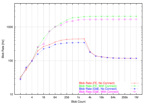
The results of the plateau measurements that have been made for the blob communication mechanism are shown in Fig. 8.28. It can be realized that for the two connected tests the rate rises steadily with the number of blocks to a plateau reached between 8 k and 32 k blocks. Unlike the message communication these tests show no peak over the measured spectrum. For the unconnected tests a similar rise is displayed which drops off again and reaches a lower plateau starting at about 8 kB. For the blob throughput tests’ evaluation of the plateau value the number of 32 k blocks was chosen as a common point of reference. A 2 k (2048) blob count was chosen for the peak values of the unconnected tests, while for the connected tests the values at 32 k blobs were reused as no real peak exists for these tests.
Plateau Throughput Measurement
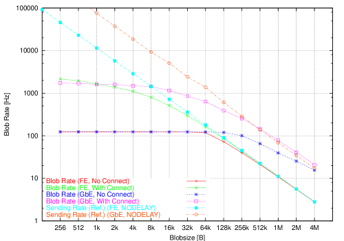
Fig. 8.29 to 8.33 display the results that have been obtained during the on-demand allocation throughput tests using a blob count of 32768 (32 k) for each size, going from 256 B to 4 MB. The first result, the achievable sending rate, is shown in Fig. 8.29. As can be seen, the maximum values are about 1.5 kHz to 2 kHz for the connected tests and about 120 Hz for the unconnected tests. In the Fast Ethernet test with explicit connections the maximum value is somewhat higher than 2 kHz, reached at the smallest block size of 256 B. With increasing block sizes the rate continously decreases. From about 16 kB to 32 kB the decrease in rate becomes linear with block size as the available network bandwidth becomes the limiting factor, as can be seen in Fig. 8.30, too. For the connected Gigabit Ethernet test an initial plateau with only a slight decrease can be observed from 256 B to 8 kB block sizes. At 8 kB blocks a steeper decrease starts which also develops into a linear decrease when the network starts to become the bottleneck. Except for the initial two values at 256 B and 512 B, where it is slightly lower than Fast Ethernet, the connected GbE test constantly shows the highest achievable sending rate, as could be expected due to its higher available bandwidth. The fact that the FE curve is higher at 256 B could be explained by its lower latency in exchanging the allocation messages which dominates the rate at these small sizes. Between 64 kB and 128 kB the unconnected Gigabit Ethernet rate starts to exceed the connected Fast Ethernet curve, which closely approaches the unconnected Fast Ethernet curve after 256 kB block sizes. For these sizes the overhead of establishing the connection for each block thus is becoming negligible compared to the sending of the large blocks. In comparison with the reference measurements one can see that the connected blob tests reach the reference values later than the corresponding message class curves. This is most likely due to the overhead of allocating a block in the remote buffer and sending of an additional message to announce the block to the receiver. But, similar to the message class, for large blocks the achieved sending rate exceeds the one of the reference benchmark. The explanation for this is the same as given in the message class section: The message class usage of preceeding the read and write calls with select class seems to be more efficient than the simple use of blocking read and write calls.
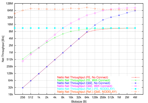
The measured network throughputs of the tests are shown in Fig. 8.30. One can see that the blob class throughput curves rise linearly with three separate slopes to a specific point for each curve. At these points the increase slows down as the hardware limit is approached, which can be seen by comparison with the reference measurements. In this comparison one can also see again that the connected GbE blob class throughput exceeds the respective reference throughput for large blocks, as already observed in the rate measurement above.
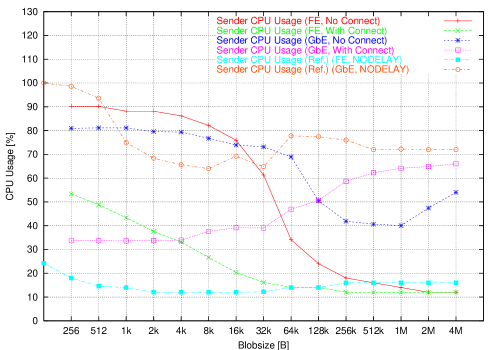
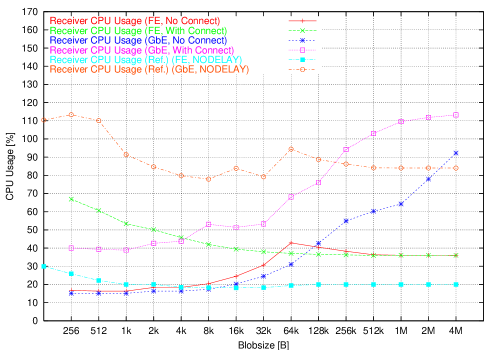
CPU usage during the blob transfers can be seen in Fig. 8.31, for the sender on the left and the receiver on the right hand side. On the sender one can see that the connected Fast and Gigabit Ethernet blob class measurements are lower than the corresponding reference measurements; the FE one for large blocks and the GbE one for the whole test range. This corresponds to behaviour already observed in the message class tests. The reason why the GbE curve displays less CPU usage even at small block sizes is very likely related to the fact that the achieved rates and throughputs at these block sizes are noticeably lower than in the reference measurements. The other notable feature in the sender graph is the very high load of the two unconnected blob measurements at small blocks. This is also similar to the observed message class behaviour and is most likely caused by the connection establishing overhead. On the receiver node the blob class connected Fast Ethernet curve is constantly at higher values than its reference counterpart. The connected GbE blob class curve is lower than the reference measurement at small block sizes and rises above it for large blocks, approximately where its rate and throughput also exceed the reference ones. At small block sizes the low usage therefore seems to be, at least in part, caused by the low sending rate and throughput values.
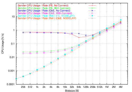
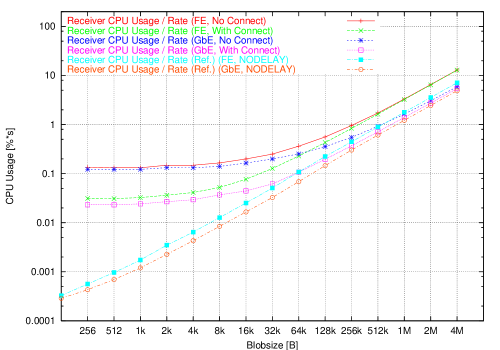
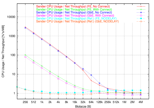
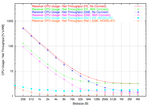
To allow a better interpretation of the CPU usage values they are normalized to the achieved blob sending rate and network throughput, similar to the message throughput tests. The results are displayed in Fig. 8.32 and Fig. 8.33 respectively. These curves are very similar in appearance to those for message sending in Fig. 8.20 and Fig. 8.21, with the exception of the higher blob class usages compared to the corresponding message classes usages. This is the case for sender and receiver, connected and unconnected, as well as Fast and Gigabit Ethernet tests. A possible explanation for this is that for each blob to be transferred three messages (block allocation request and reply as well as block announcement) have to be sent as well, which speaks in favor of the preallocation method examined below in section 8.4.5.
Peak Throughput Measurement
To measure the peak blob class throughput the implicit connection tests have been run with a blob count of 2048 (2 k) where the throughput for 256 B blocks has reached its peak value. Unlike these unconnected tests, the connected ones have not been rerun as the respective curves from Fig. 8.28 do not show a peak value. Instead the 32 k count measurements from the previous section have been used for this measurement as well. The discussion of the measurements and their differences is therefore primarily focussed on the implicit connection tests. Results that have been obtained from these measurements are shown in Fig. 8.34 to 8.38.
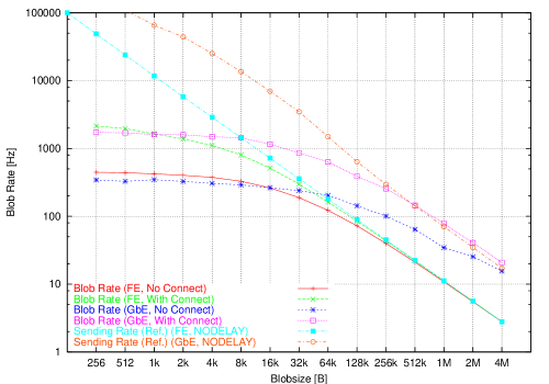
For the achieved blob sending rates shown in Fig. 8.34 it can be seen that the results for the peak tests are higher than those from the previous plateau tests of Fig. 8.29. The results of the tests differ by a factor of about 3 and 4 for the Fast and Gigabit Ethernet measurements respectively. A comparison of the connected tests with the respective reference measurements yields the same qualitative results as for the plateau test. The reference rates are reached only for relatively large blocks, but the connected GbE measurement exceeds the GbE reference curve for the largest blocks, as before. Both blob class Fast Ethernet measurements initially have higher rates than their respective Gigabit Ethernet counterpart. As for the plateau test this is again presumed to be due to Fast Ethernet’s lower latency. Since at the operating system level messages have to be exchanged for connection establishing and termination the increased latency should influence the unconnected tests more than the connected ones. This is reflected in the graph, as the connected GbE curve exceeds the connected FE curve earlier than the unconnected GbE curve exceeds the unconnected FE curve. One interesting point to be found in the plot is the transition from 1 MB to 2 MB blocks for the unconnected Gigabit Ethernet curve, where the new curve displays a bend and for large blocks becomes identical to the curve from the previous plateau measurement. The reason for this bend are presumably buffers filled by the larger blocks which causes the same behaviour for the peak test as for the plateau test.
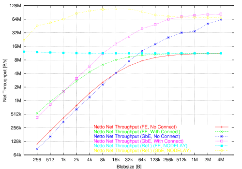
From the measurements of the application level network throughput in Fig. 8.35 the same tendencies as for the blob sending rate can be derived. The throughput for the unconnected tests is higher by factors of about 3 to 4 for small blocks up to the point where the available bandwidth becomes the limit. One can also see the bend in the unconnected GbE curve that marks the transition from the peak to the plateau throughput measurement. This bend appears even more pronounced than in the rate plot of Fig. 8.34.
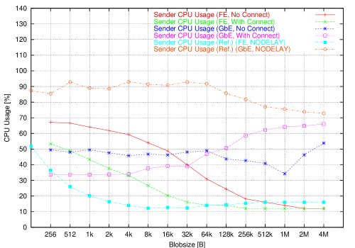
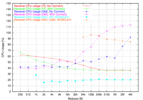
In the CPU usage measurements of the peak throughput tests in Fig. 8.36 one can see that compared to the plateau tests the sender CPU usage in general reaches lower values. For the receiver on the other hand the measured peak test usages are higher than the ones from the corresponding plateau tests. As for the previous communication class measurements it can be seen that the connected CPU usages on the sender are still lower than the reference ones; for FE only for large blocks but for GbE over the whole test range. On the receiver the plateau behaviour is also repeated. Connected FE blob class usage is always higher than the reference measurement and connected GbE usage exceeds the respective reference usage only for large blocks, approximately in the range where the class reaches a higher throughput than the reference measurement. One can also see, on the sender as well as on the receiver, that the unconnected GbE blob class measurement transitions between 512 kB and 1 MB blocks from the peak test behaviour to the same behaviour that has been exhibited in the plateau test. This is similar to what was seen in the rate and throughput measurements (Fig. 8.34 and 8.35).
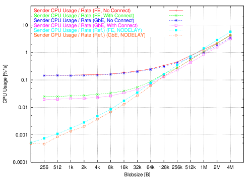
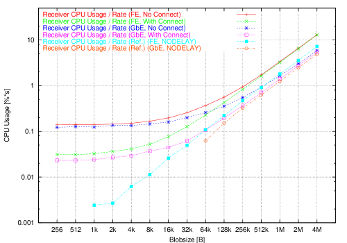
For a better comparison normalized CPU usages, i.e. CPU usage divided by the achieved rate respectively network throughput, have been plotted in Fig. 8.37 and 8.38 instead of absolute CPU usage. As can be expected due to the higher sending rates, both peak test curves show significantly lower CPU usage per rate values on the sending node compared to the corresponding plateau test results in Fig. 8.32. The improvement between the two tests is about a factor of 5 for each of the curves. An interesting point can be seen for the two curves at the end of the initial constant plateau in Fig. 8.32. After a short transition at 32 kB for FE and 128 kB for GbE the curve from the previous plateau throughput measurement becomes identical to the smoothly increasing curve from the peak throughput measurement. In this case the bend is clearly seen in the curve of the plateau tests and not the in peak tests’, as for the Gigabit Ethernet rate, network throughput, and CPU usage measurements. The reason for this behaviour has not been determined and no plausible explanation could be found in the course of this thesis. On the receiver node the curves from the two different throughput tests are nearly indistinguishable. Compared to the reference benchmarks the behaviour already observed in the preceeding communication class tests is seen: On the sender the connected FE and GbE blob class tests are better for larger blocks, while on the receiver they are less efficient over the whole test range.
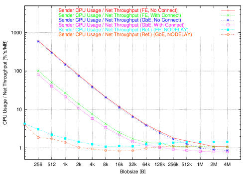
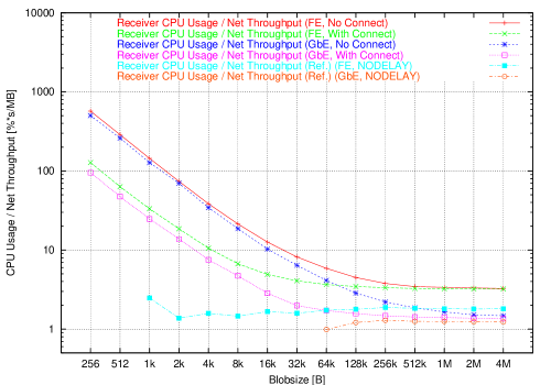
As before, the measurement of the CPU usage per network throughput shown in Fig. 8.38 results in a similar improvement factor of roughly 5 compared with the plateau throughput test in Fig. 8.33. The transition in the plateau test curve towards the smooth curve from the peak test can also be seen, although less pronounced, between the 32 kB and 64 kB and 128 kB and 256 kB blocks for Fast and Gigabit Ethernet respectively. The comparison between the blob class and the reference measurements leads to the same conclusions as discussed for the usage per rate graphs.
8.4.5 TCP Blob Class Throughput with Preallocation
As for the previous throughput measurements the benchmark for the blob class in preallocation mode also splits in two parts, the initial determination of the number of blocks (blobs) sent for each block size and the actual throughput measurement in dependence of the block size.
Plateau Determination
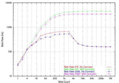
The plot of the blob sending rate in dependence of the number of blocks sent in preallocation mode is shown in Fig. 8.39. The same shapes of the curves as in the corresponding on-demand allocation tests from the previous section can be made out, although the absolute rates are higher by a factor of 2 for the connected final values, 1.5 for the peaks of the unconnected curves, and about 1.2 for their final values. As the final plateaus for the unconnected tests are reached at higher values than in the on-demand allocation rate measurements, the blob counts of 131072 (128 k) and 2048 (2 k) have been chosen for the plateau and peak measurements respectively. Since the connected curves display no peak the plateau results at 128 k messages are reused as the values for the peak tests.
Plateau Throughput Measurement
Results of the throughput plateau measurements with block counts of 128 k are displayed in Fig. 8.40 to Fig. 8.44. The rate measurements in Fig. 8.40 show the same basic shape as the equivalent curves in on-demand allocation mode from Fig. 8.29. Achieved rates are higher than in the on-demand tests though, initially about 160 Hz unconnected and 4.8 kHz connected. These rates are higher by a factor of 1.3 for the unconnected and about 3 for the connected tests respectively. For the two Gigabit Ethernet curves even the final results where the available network bandwidth already influences the rate are higher than the ones from the on-demand tests. In the Fast Ethernet measurements the two tests produce identical results from 64 kB blocks on. At these sizes the network sets the absolute limit and is not only a limiting influence as for GbE. Comparing the two connected curves one sees that in this test Gigabit Ethernet has a higher transfer rate than Fast Ethernet for all block sizes. The higher initial rate for FE in on-demand mode is thus due to the lower message latency that influences the round-trip time for the allocation messages as presumed. Since these messages are not required in preallocation mode the effect is not seen in this test. Comparing the blob class and reference measurements one can see that for larger blocks both connected curves reach the respective reference curve and in the case of Gigabit Ethernet even exceed it, as also observed in the previous communication class measurements. Absolute rates are not considerably different than in the on-demand allocation blob class measurement, since the hardware is the primary limit for large blocks, but the block sizes where the reference curves are reached or exceeded are about a factor of 2 smaller than in the on-demand allocation measurement. The performance increases, compared to the on-demand allocation measurements, should be due to the use of the preallocation mode, with its lack of the allocation request-reply message sequence.

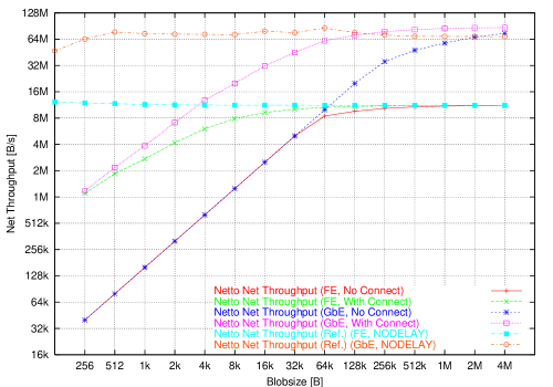
Similar results can be deduced from the network throughput measurement in Fig. 8.41. The achieved throughput is higher for all curves, with Fast Ethernet at the smaller blocksizes up to about 64 kB and with Gigabit Ethernet over the whole test range. The available bandwidth starts to limit the throughput already at about 256 kB blocks for the unconnected Fast, at 16 kB for the connected Fast, and at 256 kB for the connected Gigabit Ethernet test. Unconnected Gigabit Ethernet is not limited by the available bandwidth up to the maximum tested blocksizes of 4 MB.
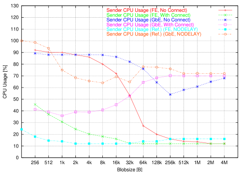
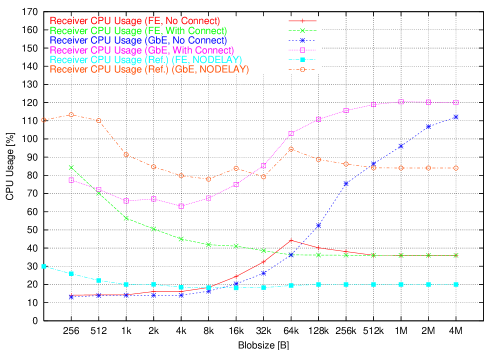
As can be seen in Fig. 8.42 the CPU usage during blob transfers on the sending node increases for both Gigabit Ethernet tests by about 5 % to 10 % over the whole test range, compared to the equivalent on-demand allocation tests. This is presumably due to the absolute higher sending rates observed in this mode. For the two Fast Ethernet measurements on the sender the opposite effect is observed. CPU usage is lower than for the equivalent on-demand allocation tests by about 5 % for smaller block sizes. This decrease is present up to the largest block sizes where the network limits the throughput and thus the CPU usage too. The FE network limit also starts to affect the tests for smaller block sizes than for the on-demand tests. The reason for this decrease is presumably caused again by the lack of the allocation request-reply messages. In addition to increasing the rate the CPU usage decreases as the additional messages do not have to be sent and received on each node. In comparison with the respective reference measurements one again can see that the communication class GbE curve is at lower values over the whole test range while the FE curve is higher, but only for small block sizes. This is identical to previously observed behaviour, and the presumed causes are similar as well. However, the communication class GbE curve approaches the reference curve closer than the GbE blob on-demand allocation measurement, due to its higher absolute usage values.
On the receiver the effect on the connected Gigabit Ethernet test is identical to that on the sender, except that on the receiver the increase is between 5 % up to almost 20 % for small blocks. For the Fast Ethernets test the opposite effect compared to the sender sets in for small block sizes, CPU usage is increased by almost 10 %. The curves for FE are again identical to those from the on-demand test at large blocks. The unconnected GbE test only shows a small increase at small block sizes of less than 5 %. With growing block sizes, though, the difference grows to about 10 % as well. These observed increases in CPU usage are most probably caused by the increases in blob rates/network throughput, as correspondingly more data has to be handled by the receiver. On the sender the increased rate does not necessarily cause a CPU usage increase, as less data, practically none, has to be received there without the allocation reply messages from the blob receiver node.
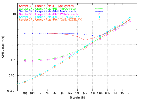
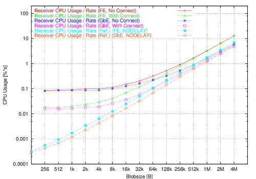
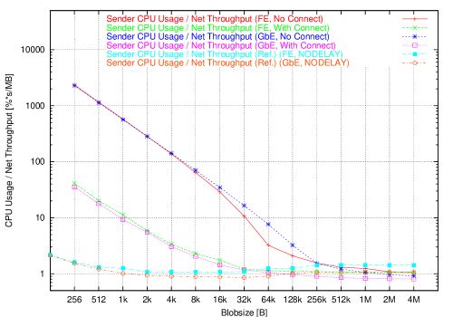
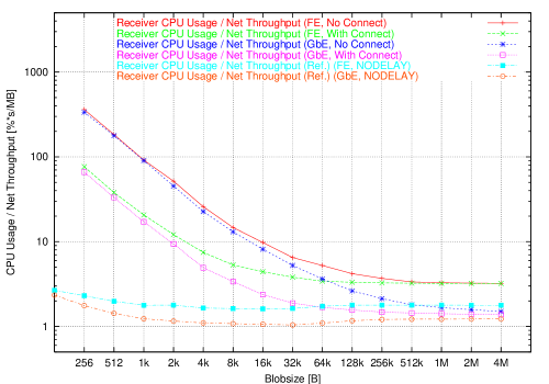
Inspecting the CPU usage normalized with the event rate and network throughput in Fig. 8.43 and 8.44 respectively, the comparison with the on-demand allocation mode is more favorable for the preallocation tests. The basic forms of the curves are identical for both measurements on the sender as well as on the receiver. In a comparison of the two transfer modes, the CPU usage to rate (or throughput) ratios of the preallocation tests are better by factors of 2.5 to 2.2 for the connected Fast and Gigabit Ethernet tests respectively and 1.25 to 1.17 for the unconnected FE and GbE measurements. These ratios are measured for 256 B blocks, towards the largest blocks the ratios become almost equal with a relative difference of only a few percent. This respective approach of the two tests’ curves can be expected, as for these large blocks the main influence is by the actual transfer itself and the allocation message exchange becomes negligible. Qualitatively the behaviour relative to the reference tests is similar to the ones of the on-demand allocation measurements. Due to the lower values in preallocation mode, however, the relative differences are distinct; when the communication class measurements are higher than the reference, the difference has become smaller and when the class measurements are lower, the difference has become larger.
Peak Throughput Measurement
The final blob class throughput measurement is performed in preallocation mode with a block count of 2048 (2 k) for the unconnected tests, with results shown in Fig. 8.45 to 8.49. As for the on-demand allocation peak throughput tests the connected plateau throughput tests with a 128 k block count from the previous section are reused here. The following discussion will therefore focus on the two unconnected tests.
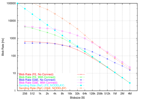
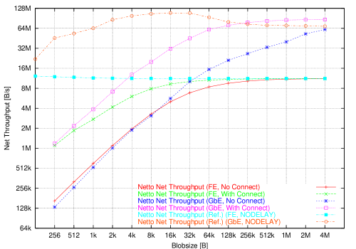
For the measured rates and network throughputs, shown in Fig. 8.45 and 8.46 respectively, the relation to the preallocation plateau throughput tests is in principle identical to the relation of the plateau and peak on-demand allocation tests. The rates (and therefore also throughput values) achieved are the highest of all four unconnected block transfer tests: a maximum rate of more than 650 Hz and 533 Hz at 256 B blocks for Fast and Gigabit Ethernet respectively. Network throughput for Fast Ethernet is higher up to about 64 kB blocks where the network bandwidth becomes the limit for all FE tests. The achieved results differ by factors of 3 to more than 4 relative to the preallocation plateau tests, and for the on-demand peak tests the factors are 1.3 to 1.4. At larger block sizes this effect is decreasing, and at the largest blocks this test has only a small advantage for Gigabit Ethernet and none for Fast Ethernet. The reasons for this increase relative to the on-demand peak test are again the lack of the request-reply allocation message sequence. With regard to the preallocation plateau test the increase is presumably caused by buffers which are able to accept a large part of the small blobs, analogous to the other peak test increases. As for the other comunication class tests the connected FE curve approaches its appropriate reference curve and the connected GbE curve exceeds it for large blocks.
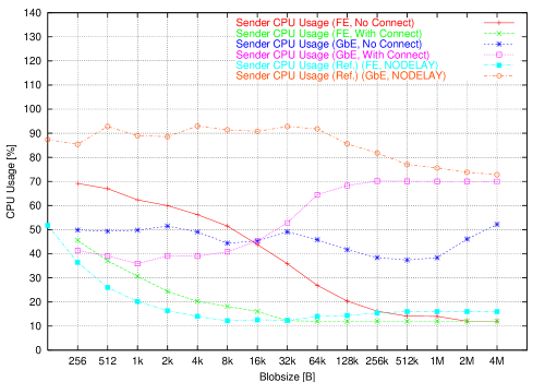
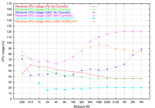
CPU usage on the sending node is displayed in Fig. 8.47. For the connected measurements it is approximately equal to the one from the preallocation plateau test described above, despite the higher rates. Concerning the unconnected tests, their usage is considerably higher at small blocks than in the plateau test, reflecting the already observed overhead of establishing connections on the initiating (or sending) node, coupled with the higher rates in this test. Compared to the on-demand peak test the usage is slightly higher, most likely because of the higher sending rates.
On the receiver measured connected usage is again roughly the same as in the preallocation plateau test and the unconnected usage is again considerably higher at small blocks. The factor for the unconnected measurements is between 3 and 4 for both tests relative to the plateau test. Compared to the on-demand allocation peak tests the results are identical or higher, up to a factor of 2 for the connected GbE curve at small block sizes. This increase is again caused most probably by the increase in sending rate relative to the on-demand test. Where measurements are available both connected measurements considerably exceed their respective reference measurement, at least in part due to the additional block announcement message which has to be received by the communication class, as already discussed.

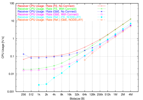
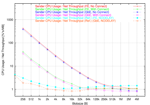
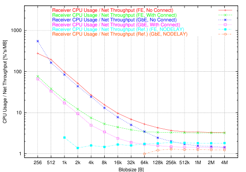
In the efficiency comparison of CPU usage per rate respectively network throughput, the curves on both sender and receiver have almost identical forms in the two peak throughput tests, with the results of the preallocation mode tests at lower (and better) values. For small block sizes the preallocation test results are better by a factor of about 1.5 for the two unconnected tests and by a factor of about 2.3 for the connected ones. With growing block sizes the difference between the tests becomes smaller. On a small scale the results are even reversed so that the on-demand test partially has better values. At the largest block sizes the difference between the tests is at most 1 % for the unconnected tests in favour of the preallocation tests. For the connected tests at these block sizes the on-demand allocation mode tests are better by about 0.5 % to 2 %. As the block sizes increase the block’s actual transfer increasingly dominates the overhead and the difference caused by the different allocation messages becomes smaller and smaller, causing the different tests’ results to become similar. A possible explanation for the on-demand allocation test’s efficiency being higher than the preallocation test’s could be that in preallocation mode buffer can be filled more quickly, due to the missing allocation sequence latency. Therefore buffers can also overflow more quickly, leading to packet losses and retransmits. These retransmits do not increase the throughput but still have to be processed, decreasing the transfer’s efficiency. The effect is probably not seen in the plateau tests’ due to the larger amount of data transferred, causing overflows in both allocation modes. On the other hand, these differences are not large and could therefore just be noise respectively measurement uncertainties.
8.4.6 TCP Blob Class Latency with On-Demand Allocation
To determine the latency of the TCP blob class, measurements similar to those for the message class from section 8.4.2 have been executed in on-demand mode. Corresponding measurements in preallocation mode are described in section 8.4.7. In this test varying numbers of data blocks are transferred from sender to receiver. After each block the sender waits for the block to be sent back by the receiver before continuing with the next block. Fig. 8.50 shows the results that have been obtained from this ping-pong pattern.
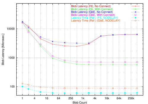
As can be seen in the figure, the latency curves display the same general pattern as those for messages in Fig. 8.27. A sharp decrease turns into a plateau and rises sharply to a second plateau in the unconnected tests. The jump to the second plateau in the unconnected tests sets in at lower counts than for the message tests, between 2 k and 8 k for the blobs compared to between 8 k and 32 k for messages. In comparison with the message tests the plateaus are at higher values. These higher values are to be expected as sending a blob with on-demand allocation requires the sending of three messages on both nodes, two for the buffer space allocation and one for the notification that a blob is available. Similar to the message tests and also as expected the unconnected tests display again much higher latencies compared to the connected tests. The jump between the two unconnected test plateaus is just by a factor of 2 instead of 2.5 as found in the message test.
| Fast | Fast | Gigabit | Gigabit | Fast | Gigabit | |
| Ethernet | Ethernet | Ethernet | Ethernet | Ethernet | Ethernet | |
| Implicit | Explicit | Implicit | Explicit | Reference | Reference | |
| Connect | Connect | Connect | Connect | |||
| Minimum Average Blob | 2470 | 570 | 3190 | 700 | 61 | 88 |
| Latency / | ||||||
| Minimum Average Blob | 1413 | 240 | 2080 | 344 | - | - |
| Latency / | ||||||
| w/o Message Latencies |
Table 8.10 summarizes the minimum latency times measured for each of the four different configurations. Each connected test is about 4.5 times faster than the respective unconnected test, and the Fast Ethernet tests are between 23 % (connected) and 29 % (unconnected) faster than their corresponding Gigabit test counterparts, in each case a higher relative difference than in the message latency tests. Compared to the reference measurements the latencies are considerably increased, almost by an order of magnitude for the connected and about a factor of 40 for the unconnected tests. One part of the explanation for this is most definitely the fact that three times the respective message latency (allocation request, allocation reply, blob announcement) is included in these times. When these message latencies are subtracted the remaining “pure” blob latencies are considerably lower, but still higher than the message and in particular the reference latencies. This can in part be caused by the larger block used in the blob test, 256 B instead of 8 B for the reference and 32 B for the message class. A second potential cause can be the 32 bit value that is written back to the sender by the receiver blob class after each transfer, to indicate completion, which contributes approximately one respective reference latency to the blob latency.
8.4.7 TCP Blob Class Latency with Preallocation
The same test as in section 8.4.6 has been performed for the blob classes in preallocation mode as well, with the results shown in Fig. 8.51. As can be seen the shape of the four curves is as good as identical to the ones in the on-demand allocation latency measurements in Fig. 8.50. A major difference between the plots is that the values in preallocation mode are lower than those in on-demand allocation mode, which also can be seen when comparing Table 8.11 and Table 8.10. The unconnected tests are faster roughly by a factor of 1.5, the connected ones even by a factor of about 1.8, compared to the values from the on-demand allocation tests. For the preallocation values themselves a comparison of the unconnected and connected tests yields factors of 5.1 and 5.4 for Fast and Gigabit Ethernet respectively. Compared to Gigabit Ethernet, Fast Ethernet is about 22 % and 29 % faster for connected and unconnected tests respectively, basically identical to the on-demand allocation latency differences. Relative to the reference latency results the measured latencies are still fairly high. Taking into account the latency corresponding to the one remaining message (blob announcement), the resulting “pure” times are identical to a first approximation with the respective times in on-demand allocation mode. In preallocation mode, however, all values are slightly lower. These time differences could be due to the added allocation and release functionality that has to be executed locally on the receiver in on-demand allocation mode.
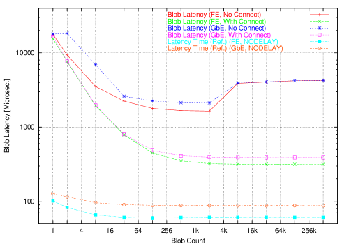
| Fast | Fast | Gigabit | Gigabit | Fast | Gigabit | |
| Ethernet | Ethernet | Ethernet | Ethernet | Ethernet | Ethernet | |
| Implicit | Explicit | Implicit | Explicit | Reference | Reference | |
| Connect | Connect | Connect | Connect | |||
| Minimum Average Blob | 1640 | 320 | 2120 | 390 | 61 | 88 |
| Latency / | ||||||
| Minimum Average Blob | 1290 | 210 | 1750 | 271 | - | - |
| Latency / | ||||||
| w/o Message Latencies |
8.4.8 TCP Blob Benchmark Summary
The primary conclusion to be drawn for the TCP blob classes is that, just as the message classes, they are able to handle the requirements presented by the ALICE HLT within the scope of the current hardware used in the tests. The requirements are particularly fulfilled in preallocation mode, as it is used in the framework’s bridge components. In heavy-ion mode average block sizes of around 300 kB are expected for the largest parts of data, the ADC values read-out from the detector. At these block sizes the classes are still able to handle a rate of more than the required 200 Hz over Gigabit Ethernet. The 1 kHz rate required for operation in pp mode is possible up to 64 kB large blocks. These evaluations all refer to the connected mode, as the blob classes will not be used with implicit connections in the HLT. A reduction of CPU usage during transfers is still desirable, and it should also be achievable to a certain degree by more powerful CPUs and more efficient network adapters. But optimization potential in this respect should also still exist in the communication library itself so that further tuning measures of its classes can be undertaken as well.
Just as for the message classes, if latency is of lesser importance, the use of Gigabit Ethernet recommends itself due to the lower relative CPU usage values per network throughput, even when the absolute throughput required does not necessitate its use. If latency is a concern, the use of Fast Ethernet is suggested whenever possible because its latencies are lower than those of Gigabit. For the framework components this is of no concern as the conditions allow to treat latency with secondary priority. For the HLT the amount of data to be transferred over the network, however, implies the use of at least Gigabit Ethernet even without its efficiency advantages. Since the sizes of the different types of data passed between the HLT’s stages are not yet known, predictions of the CPU usage incurred by the transfers cannot be made at the current stage.
A direct comparison with the network reference measurements reveals similar results as in the message class – reference comparison. Again the first noticeable details are the different characteristics in the graphs showing rate as a function of count. For the connected tests the decrease is not present at all, while in the unconnected ones it is again more obvious than in the reference tests. As far as latency is concerned, this is considerably increased in the blob classes because of the need to send the blob data itself as well as the message informing the receiver about the transmission. Results from the plateau and peak throughput tests are shown in a summary in Tables 8.12 and 8.13 respectively. In the following discussion only the connected tests are regarded, as the results of the unconnected ones are considerably poorer in turn. Concerning the achieved block sending rate the reference tests are mostly much faster, particularly for small block sizes. The respective differences are actually between one and two orders of magnitude. An exception are the Gigabit Ethernet measurements at the largest block sizes, where the minimum achieved rates, with the blob measurements are slightly higher than those for the reference’s. For the network throughput the reference tests consistently show better values than each of the blob tests, at least for the minimum and maximum values listed in the tables. As a further exception the GbE measurements of CPU usage and efficiency for sender and receiver differ from the expected characteristics that the reference tests always results in lower values. These differences also vary between the plateau and peak throughput tests. In the plateau measurements the absolute CPU usages for GbE are always lower on the sender, while for the efficiency the minimum values at large block sizes are lower. On the receiver the absolute CPU usage minima are lower, and maxima are roughly equal or slightly higher. As expected, efficiency values on the receiver are always higher than in the reference tests. In the peak tests only values on the sender are better in the blob tests. Absolute CPU usage is always better for the blob classes, while for the efficiency only the minimum values are lower. The conclusion that can be drawn is also quite similar to the one for the message classes. Some of the overhead and performance loss in the blob classes certainly has to be accepted as part of the added functionality and in particular flexibility compared to the simple reference test program. However, the potential for optimization is definitely greater than in the message classes, as can be seen in the considerably lower sending rates of the blob classes compared with the message class rates, so that the need for tuning measures is a definite must. The efficiency measurements that, at least on the sender, indicate better results compared to the reference program, again stand out positively, with the same possible explanation as for the message class.
| Rate / | Network | CPU Usage | CPU Usage | CPU Usage / | CPU Usage / | CPU Usage / | CPU Usage / | |
|---|---|---|---|---|---|---|---|---|
| Measurement | Hz | Throughput / | Sender / | Receiver / | Rate | Rate | Throughput | Throughput |
| Type | % | % | Sender / | Receiver / | Sender / | Receiver / | ||
| Reference | 2.8 @ 4 M | 11.2 @ 256 | 12 @ 2 k | 18.1 @ 16 k | 0.000392 | 0.000563 | 1.07 @ 16 k | 1.62 @ 16 k |
| FE w. | 45900 @ 256 | 11.2 @ 4 M | 18 @ 256 | 25.9 @ 256 | @ 256 | @ 256 | 1.61 @ 256 | 2.31 @ 256 |
| TCP_NODELAY | 6130 | 11.2 | 14.3 | 20 | 5.7 @ 4 M | 7.13 @ 4 M | 1.28 | 1.79 |
| 0.756 | 0.95 | |||||||
| Reference | 2.8 @ 4 M | 11.2 @ 256 | 12 @ 2 k | 18.1 @ 16 k | 0.000392 | 0.000563 | 1.07 @ 32 k | 1.62 @ 16 k |
| FE w/o | 45900 @ 256 | 11.2 @ 2 M | 18 @ 256 | 25.9 @ 256 | @ 256 | @ 256 | 1.61 @ 256 | 2.31 @ 256 |
| TCP_NODELAY | 6130 | 11.2 | 14.1 | 20.6 | 5.52 @ 4 M | 7.67 @ 4 M | 1.26 | 1.83 |
| 0.744 | 1.02 | |||||||
| Reference | 17.1 @ 4 M | 64.3 @ 256 | 64 @ 8 k | 77.9 @ 8 k | 0.000374 | 0.00043 | 0.854 @ 32 k | 1.04 @ 32 k |
| GbE w. | 264 k @ 256 | 86.2 @ 64 k | 98.6 @ 256 | 113 @ 256 | @ 256 | @ 256 | 1.53 @ 256 | 1.76 @ 256 |
| TCP_NODELAY | 38200 | 73.1 | 74.6 | 88.4 | 4.2 @ 4 M | 4.9 @ 4 M | 1.03 | 1.21 |
| 0.558 | 0.651 | |||||||
| Reference | 17.1 @ 4 M | 64.3 @ 256 | 66.4 @ 8 k | 80.8 @ 8 k | 0.000364 | 0.000427 | 0.866 @ 32 k | 1.04 @ 32 k |
| GbE w/o | 263 k @ 256 | 88.4 @ 64 k | 96 @ 256 | 113 @ 256 | @ 256 | @ 256 | 1.49 @ 256 | 1.75 @ 256 |
| TCP_NODELAY | 38600 | 74.4 | 75.8 | 89.5 | 4.2 @ 4 M | 4.9 @ 4 M | 1.03 | 1.21 |
| 0.56 | 0.651 | |||||||
| Blob Class | 2.8 @ 4 M | 0.522 @ 256 | 12 @ 4 M | 35.9 @ 512 k | 0.0248 | 0.0309 | 1.07 @ 4 M | 3.22 @ 4 M |
| On-Demand | 2140 @ 256 | 11.2 @ 4 M | 53.2 @ 256 | 66.9 @ 256 | @ 256 | @ 512 | 102 @ 256 | 128 @ 256 |
| Alloc. | 678 | 7.32 | 24.4 | 43.3 | 4.28 @ 4 M | 12.9 @ 4 M | 14.5 | 19.5 |
| FE w. Connect | 0.59 | 1.74 | ||||||
| Blob Class | 2.78 @ 4 M | 0.0303 @ 256 | 12 @ 4 M | 16.3 @ 1 k | 0.288 | 0.132 | 1.08 @ 4 M | 3.24 @ 4 M |
| On-Demand | 124 @ 512 | 11.1 @ 4 M | 90.4 @ 512 | 42.8 @ 64 k | @ 64 k | @ 512 | 2980 @ 256 | 553 @ 256 |
| Alloc. | 84.1 | 5.18 | 53 | 28.5 | 4.32 @ 4 M | 12.9 @ 4 M | 392 | 76.1 |
| FE w/o Connect | 0.998 | 1.85 | ||||||
| Blob Class | 20.8 @ 4 M | 0.42 @ 256 | 33.6 @ 1 k | 38.9 @ 1 k | 0.0198 | 0.0232 | 0.792 @ 4 M | 1.36 @ 4 M |
| On-Demand | 1720 @ 256 | 83.4 @ 4 M | 66 @ 4 M | 113 @ 4 M | @ 256 | @ 512 | 80.2 @ 256 | 95.1 @ 256 |
| Alloc. | 874 | 35.7 | 26.6 | 69.2 | 3.16 @ 4 M | 5.43 @ 4 M | 11.5 | 13.9 |
| GbE w. Connect | 0.444 | 0.749 | ||||||
| Blob Class | 15.6 @ 4 M | 0.0302 @ 256 | 40 @ 1 M | 15.1 @ 1 k | 0.418 | 0.122 | 0.866 @ 4 M | 1.48 @ 4 M |
| On-Demand | 124 @ 256 | 62.4 @ 4 M | 81.4 @ 512 | 92.2 @ 4 M | @ 256 k | @ 256 | 2680 @ 256 | 500 @ 256 |
| Alloc. | 98.6 | 16.1 | 64.8 | 37.6 | 3.46 @ 4 M | 5.91 @ 4 M | 356 | 68.5 |
| GbE w/o Connect | 0.896 | 0.921 | ||||||
| Blob Class | 2.8 @ 4 M | 1.1 @ 256 | 12 @ 4 M | 36 @ 4 M | 0.0098 | 0.0185 | 1.07 @ 4 M | 3.21 @ 4 M |
| Prealloc. | 4510 @ 256 | 11.2 @ 4 M | 45.6 @ 256 | 84.3 @ 256 | @ 512 | @ 512 | 41.4 @ 256 | 76.5 @ 256 |
| FE w. Connect | 1140 | 8.03 | 19.2 | 45.4 | 4.28 @ 4 M | 12.8 @ 4 M | 6.32 | 12.7 |
| 0.578 | 1.73 | |||||||
| Blob Class | 2.79 @ 4 M | 0.039 @ 256 | 12 @ 4 M | 14.1 @ 256 | 0.202 | 0.0882 | 1.08 @ 4 M | 3.23 @ 4 M |
| Prealloc. | 160 @ 1 k | 11.2 @ 4 M | 92 @ 256 | 44.3 @ 64 k | @ 64 k | @ 256 | 2360 @ 256 | 361 @ 256 |
| FE w/o Connect | 105 | 5.48 | 51.6 | 27.8 | 2.3 @ 4 M | 12.9 @ 4 M | 308 | 51.4 |
| 0.886 | 1.8 | |||||||
| Blob Class | 21.7 @ 4 M | 1.17 @ 256 | 35.8 @ 1 k | 63.1 @ 4 k | 0.0086 | 0.0161 | 0.806 @ 4 M | 1.38 @ 4 M |
| Prealloc. | 4810 @ 256 | 86.8 @ 4 M | 70.2 @ 256 k | 120 @ 1 M | @ 256 | @ 256 | 35.2 @ 256 | 65.9 @ 256 |
| GbE w. Connect | 1890 | 45 | 54.4 | 92.2 | 3.22 @ 4 M | 5.53 @ 4 M | 5.46 | 9.91 |
| 0.442 | 0.756 | |||||||
| Blob Class | 18.6 @ 4 M | 0.039 @ 256 | 54 @ 256 k | 13.1 @ 256 | 0.38 | 0.0819 | 0.912 @ 4 M | 1.5 @ 4 M |
| Prealloc. | 160 @ 1 k | 74.5 @ 4 M | 89.2 @ 256 | 112 @ 4 M | @ 256 k | @ 256 | 2280 @ 256 | 336 @ 256 |
| GbE w/o Connect | 130 | 21.5 | 76.2 | 46.5 | 3.64 @ 4 M | 6.02 @ 4 M | 302 | 47.6 |
| 0.858 | 0.91 |
| Rate / | Network | CPU Usage | CPU Usage | CPU Usage / | CPU Usage / | CPU Usage / | CPU Usage / | |
|---|---|---|---|---|---|---|---|---|
| Measurement | Hz | Throughput / | Sender / | Receiver / | Rate | Rate | Throughput | Throughput |
| Type | % | % | Sender / | Receiver / | Sender / | Receiver / | ||
| Reference | 2.8 @ 4 M | 11.2 @ 4 M | 12.2 @ 8 k | 15.6 @ 2 k | 0.000746 | 0.00242 @ 1 k | 1.08 @ 8 k | 1.38 @ 2 k |
| FE w. | 48800 @ 256 | 11.9 @ 256 | 36.4 @ 256 | 28.3 @ 1 k | @ 256 | 7.24 @ 4 M | 3.06 @ 256 | 2.48 @ 1 k |
| TCP_NODELAY | 6400 | 11.3 | 17.2 | 19.7 | 5.72 @ 4 M | 1.11 | 1.51 | 1.75 |
| 0.758 | ||||||||
| Reference | 2.8 @ 4 M | 11.2 @ 4 M | 12 @ 16 k | 15.6 @ 2 k | 0.000742 | 0.00238 @ 1 k | 1.07 @ 16 k | 1.38 @ 2 k |
| FE w/o | 50400 @ 256 | 12.3 @ 256 | 37.4 @ 256 | 27.9 @ 1 k | @ 256 | 7.38 @ 4 M | 3.04 @ 256 | 2.44 @ 1 k |
| TCP_NODELAY | 6500 | 11.3 | 16.9 | 19.9 | 5.36 @ 4 M | 1.12 | 1.48 | 1.77 |
| 0.7.18 | ||||||||
| Reference | 17.2 @ 4 M | 45.6 @ 256 | 72.8 @ 4 M | 84.8 @ 4 M | 0.000458 | 0.0619 @ 64 k | 0.834 @ 16 k | 0.991 @ 64 k |
| GbE w. | 187 k @ 256 | 109 @ 16 k | 93 @ 4 k | 96.6 @ 128 k | @ 256 | 4.94 @ 4 M | 1.88 @ 256 | 1.29 @ 256 k |
| TCP_NODELAY | 30500 | 79.8 | 85.4 | 90.3 | 4.24 @ 4 M | 1.4 | 1.13 | 1.21 |
| 0.568 | ||||||||
| Reference | 17.1 @ 4 M | 63.9 @ 256 | 72 @ 1 M | 81.6 @ 512 | 0.000376 | 0.000506 | 0.872 @ 32 k | 1.04 @ 512 |
| GbE w/o | 262 k @ 256 | 106 @ 8 k | 102 @ 1 k | 113 @ 8 k | @ 256 | @ 512 | 1.54 @ 256 | 1.23 @ 512 k |
| TCP_NODELAY | 40800 | 80.7 | 84.2 | 92.9 | 4.2 @ 4 M | 4.83 @ 4 M | 1.06 | 1.14 |
| 0.56 | 0.69 | |||||||
| Blob Class | 2.8 @ 4 M | 0.522 @ 256 | 12 @ 4 M | 35.9 @ 512 k | 0.0248 | 0.0309 | 1.07 @ 4 M | 3.22 @ 4 M |
| On-Demand | 2140 @ 256 | 11.2 @ 4 M | 53.2 @ 256 | 66.9 @ 256 | @ 256 | @ 512 | 102 @ 256 | 128 @ 256 |
| Alloc. | 678 | 7.32 | 24.4 | 43.3 | 4.28 @ 4 M | 12.9 @ 4 M | 14.5 | 19.5 |
| FE w. Connect | 0.59 | 1.74 | ||||||
| Blob Class | 2.78 @ 4 M | 0.122 @ 256 | 12 @ 4 M | 36.3 @ 4 M | 0.15 | 0.139 | 1.08 @ 4 M | 3.26 @ 4 M |
| On-Demand | 500 @ 256 | 11.1 @ 4 M | 75.2 @ 256 | 62.2 @ 256 | @ 256 | @ 256 | 616 @ 256 | 571 @ 256 |
| Alloc. | 229 | 5.83 | 42.4 | 48.1 | 4.32 @ 4 M | 13 @ 4 M | 83.6 | 79 |
| FE w/o Connect | 0.364 | 1.86 | ||||||
| Blob Class | 20.8 @ 4 M | 0.42 @ 256 | 33.6 @ 1 k | 38.9 @ 1 k | 0.0196 | 0.0232 | 0.792 @ 4 M | 1.36 @ 4 M |
| On-Demand | 1720 @ 256 | 83.4 @ 4 M | 66 @ 4 M | 113 @ 4 M | @ 256 | @ 512 | 80.2 @ 256 | 95.1 @ 256 |
| Alloc. | 874 | 35.7 | 46.6 | 69.2 | 3.16 @ 4 M | 5.43 @ 4 M | 11.5 | 13.9 |
| GbE w. Connect | 0.444 | 0.749 | ||||||
| Blob Class | 15.7 @ 4 M | 0.0915 @ 256 | 34.6 @ 1 M | 41.1 @ 4 k | 0.153 | 0.123 | 0.86 @ 4 M | 1.48 @ 4 M |
| On-Demand | 378 @ 1 k | 62.8 @ 4 M | 54 @ 4 M | 92.3 @ 4 M | @ 1 k | @ 256 | 590 @ 256 | 502 @ 256 |
| Alloc. | 216 | 17.1 | 48.6 | 52.6 | 3.44 @ 4 M | 5.91 @ 4 M | 80 | 69.7 |
| GbE w/o Connect | 0.61 | 0.922 | ||||||
| Blob Class | 2.8 @ 4 M | 1.1 @ 256 | 12 @ 4 M | 36 @ 4 M | 0.0098 | 0.0185 | 1.07 @ 4 M | 3.21 @ 4 M |
| Prealloc. | 4510 @ 256 | 11.2 @ 4 M | 45.6 @ 256 | 84.3 @ 256 | @ 512 | @ 512 | 41.4 @ 256 | 76.5 @ 256 |
| FE w. Connect | 1140 | 8.03 | 19.2 | 45.4 | 4.28 @ 4 M | 12.8 @ 4 M | 6.32 | 12.7 |
| 0.578 | 1.73 | |||||||
| Blob Class | 2.79 @ 4 M | 0.161 @ 256 | 12 @ 4 M | 36.3 @ 4 M | 0.1.03 | 0.0673 | 1.08 @ 4 M | 3.25 @ 4 M |
| Prealloc. | 660 @ 256 | 11.2 @ 4 M | 69.2 @ 256 | 60.9 @ 512 | @ 1 k | @ 256 | 428 @ 256 | 276 @ 256 |
| FE w/o Connect | 281 | 6.09 | 37.4 | 45.8 | 4.3 @ 4 M | 13 @ 4 M | 58.4 | 47 |
| 0.682 | 1.83 | |||||||
| Blob Class | 21.7 @ 4 M | 1.17 @ 256 | 35.8 @ 1 k | 63.1 @ 4 k | 0.0086 | 0.0161 | 0.806 @ 4 M | 1.38 @ 4 M |
| Prealloc. | 4810 @ 256 | 86.8 @ 4 M | 70.2 @ 256 k | 120 @ 1 M | @ 256 | @ 256 | 35.2 @ 256 | 65.9 @ 256 |
| GbE w. Connect | 1890 | 45 | 54.4 | 92.2 | 3.22 @ 4 M | 5.53 @ 4 M | 5.46 | 9.91 |
| 0.442 | 0.756 | |||||||
| Blob Class | 15.3 @ 4 M | 0.13 @ 256 | 37.4 @ 512 k | 40.2 @ 8 k | 0.0934 | 0.08 | 0.85 @ 4 M | 1.44 @ 4 M |
| Prealloc. | 533 @ 256 | 61.4 @ 4 M | 52.2 @ 4 M | 88.5 @ 4 M | @ 256 | @ 512 | 382 @ 256 | 548 @ 256 |
| GbE w/o Connect | 289 | 18.2 | 45.8 | 55 | 3.4 @ 4 M | 5.77 @ 4 M | 52.4 | 60.3 |
| 0.556 | 0.87 |
8.4.9 TCP Communication Class Benchmark Summary
As an overall summary for the two types of TCP communication classes one can repeat the separate communication classes’ conclusions that they are suited for use in the ALICE High Level Trigger in the present version, even though some room for optimization is still present. The separation into different classes, optimized for small and large transfers, does not produce significant advantages in the tested version if both types of communication are handled by the same physical communication medium. An advantage might be seen when the message communication is run over Fast Ethernet, utilizing its lower latency, and the blob communication over Gigabit Ethernet using the higher bandwidth and better efficiency. One further reason why the separation does not produce any clearly visible effects could also be found in the fact that the current implementations of the communication code are not yet optimized enough for each of their specific tasks. Additionally, the combination of Gigabit Ethernet and the TCP network protocol does not provide enough features that allow to optimize for transfer efficiency. Also, TCP is not able to take enough advantage of many features provided by the networking hardware. The use of other network protocols and technologies could therefore provide clearer effects of the separation. Possible optimization measures for the communication classes are the use of the writev Linux system call that allows to pass several blocks to write into a connection socket in one system call as well as the reduction of memory allocation and release calls in the message classes. Preliminary tests of these modifications in the publisher-subscriber interface from section 6 indicate good benefits from these measures as described below in section 8.5.3.
Although all the above measurements are of course highly specific for each network device on which the corresponding test was executed, the results indicate for message as well as for blob classes that depending on the optimization goal, e.g. throughput, absolute CPU usage, or CPU usage relative to throughput, different block or message sizes are the optimum choice. The largest block size is not necessarily always the best choice.
8.5 Publisher-Subscriber Interface Benchmarks
8.5.1 Timing Measurements
To evaluate the performance of the publisher-subscriber framework and provide data and estimates of the current and expected future overhead incurred by the framework, a number of measurements have been performed. A set of benchmark publisher and subscriber programs has been written to execute the basic functions associated with announcing and freeing events only. No additional functionality, e.g. shared memory mapping or accessing, is contained in these programs. The tests have been performed on the three reference PCs evaluated and described in section 8.1.2 to obtain measurements about the scaling properties of the software. All benchmarks have been performed with almost no user processes or daemons running on the system to exclude interference effects from other processes, e.g. (de-) scheduling, as far as possible. The list of remaining processes is shown in appendix A.2.
In the two benchmark processes four different parts of the framework have been instrumented for timing measurements using the gettimeofday system call that delivers a microsecond resolution. The timing overhead of a gettimeofday call itself is small. In a test program on an 800 MHz PC the time needed to execute 100000 calls was 61275 , so one call requires about 600 ns.
The four benchmarked parts of the framework are executed for each event, as it is announced to a subscriber and released again, as detailed in chapter 6:
-
•
The main publisher object’s AnnounceEvent function that stores an event’s management data into the publisher’s internal tables and dispatches the data’s descriptor to the write threads for each subscriber.
-
•
The write thread’s function that writes the data into the named pipe.
-
•
The NewEvent function in the subscriber that writes the data release message (EventDone) into the pipe to the publisher.
-
•
The publisher’s EventDone function that releases the event management data from its internal tables.
One of the principal problems of measuring a program’s (processing) overhead is that a program’s running time for a particular code section does not provide an adequate measure of its overhead. This inadequacy results from the fact that a program may be suspended while executing the section, increasing the section’s runtime but not the overhead. Reasons for a suspension might be that the operating system deschedules it, allowing other programs to execute, or because it has to wait for an operation to complete, e.g. disk or network I/O, or for a lock to become available. While the case of explicit sleeps can in principle be accounted for during measurement by deducting the corresponding sleep time from the runtime, the other cases cannot be predicted. Even in the explicit sleep case there are problems, as the operating system may let a program sleep longer than the specified time. Therefore a way has to be found to exclude these sleep times from the overhead measurement for a given program, as these represent time where the active thread sleeps and thus does not use the CPU producing overhead.
In the publisher-subscriber measurements lock calls have been excluded from the timing, by starting and stopping the timing measurement before and after it explicitly. For the other cases the presumption can be made that code section runtimes during which a program has been suspended, which therefore are unsuitable for overhead measurements, will be significantly longer than those where the section could be executed uninterrupted. These longer values can then be excluded from the overhead measurement. A precondition for this is of course that the examined code sections are sufficiently short so that a minimal descheduling will actually be longer than a normal section execution.
events have been processed on each of the three PCs and the four timing values for each event have been entered into a runtime histogram for later analysis. For the analysis a cut-off has been made so that the contents of the bins used for the analysis amount to at least 90 % of the histogram entries. This cut-off is made under the assumption, detailed above, that longer times only occur when the examined process is inactive, which has no influence on the framework’s overhead. The mean values with and without the cut-off are shown in Table 8.14, all values are in microseconds. For both mean values the scaling constants from 733 MHz to 800 MHz and 800 MHz to 933 MHz are shown as well. The complete timing analysis plots are shown in Fig. 8.52, 8.53, 8.54, and 8.55, containing the superimposed time distribution for the three reference PCs, 733 MHz values in green, 800 MHz values in blue, and 933 MHz values in red. 800 MHz and 933 MHz values are scaled with factors of and respectively for clarity. Each plot also shows the respective bins where the 90 % cut-off was made. As can be seen from the times which make up the majority of the measurements, the values presumed to be descheduled are indeed significantly longer than the majority.
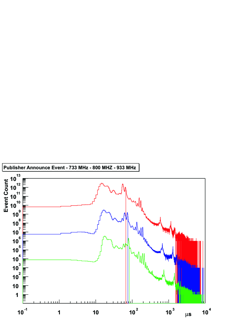
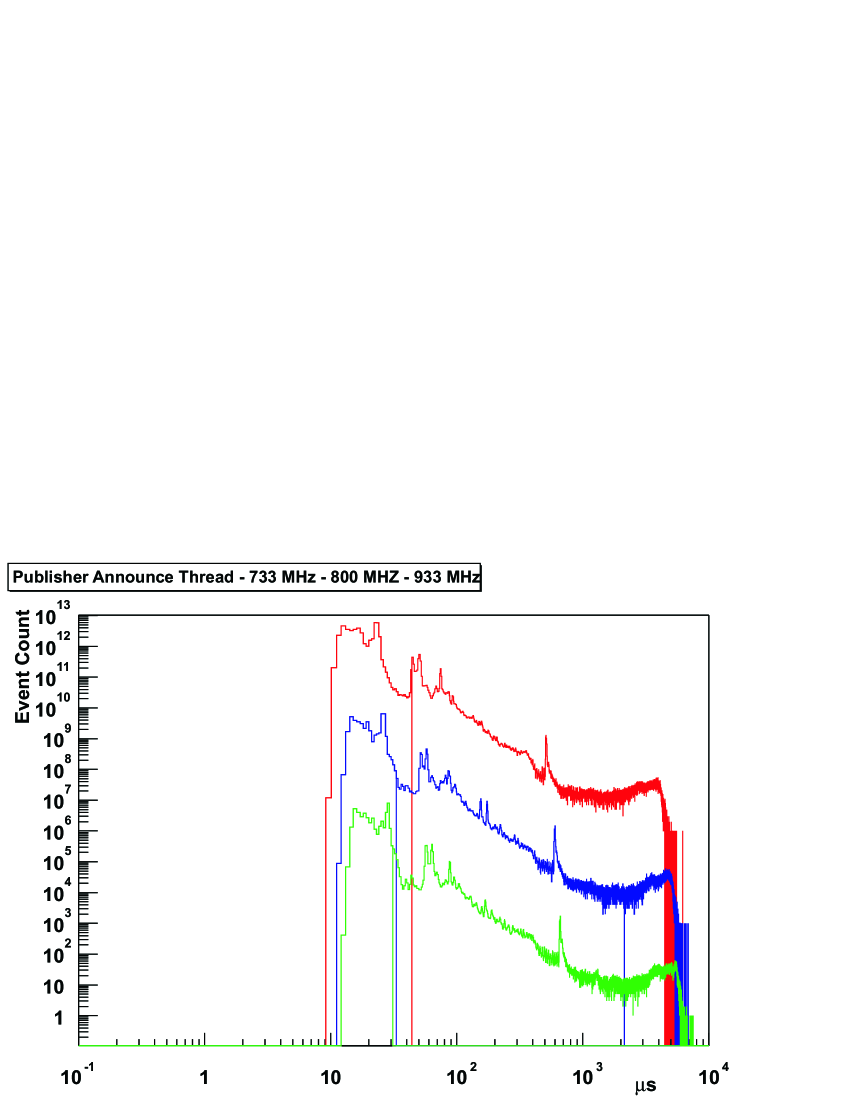
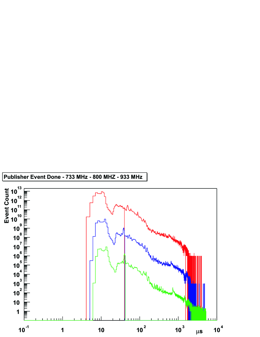
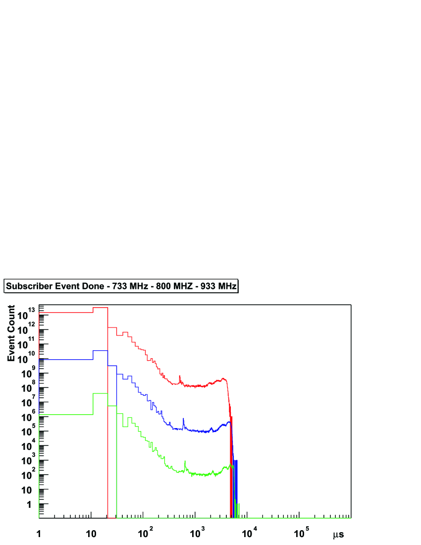
| 733 MHz | 800 MHz | 933 MHz | scaling | scaling | |
| PC | PC | PC | 733-800 | 800-933 | |
| event announce / | 50.20 | 47.42 | 42.55 | 1.06 | 1.11 |
| event announce | 40.89 | 39.21 | 35.73 | 1.04 | 1.10 |
| (cut-off) / | |||||
| announce thread / | 35.73 | 32.51 | 27.95 | 1.00 | 1.16 |
| announce thread | 21.98 | 20.68 | 18.41 | 1.06 | 1.12 |
| (cut-off) / | |||||
| publisher event done / | 22.82 | 20.46 | 17.85 | 1.12 | 1.15 |
| publisher event done | 15.52 | 13.82 | 11.56 | 1.12 | 1.20 |
| (cut-off) / | |||||
| subscriber event done / | 26.67 | 22.06 | 18.52 | 1.21 | 1.19 |
| subscriber event done | 15.86 | 13.88 | 11.88 | 1.14 | 1.17 |
| (cut-off) / | |||||
| total / | 135.45 | 122.45 | 106.87 | 1.11 | 1.15 |
| total (cut-off) / | 94.25 | 87.59 | 77.58 | 1.08 | 1.13 |
A final measurement that has been performed is the global average announce rate that can be sustained over the events. These values are shown for the three different PCs with the derived time overheads () in Table 8.15. The average processing overhead is scaled by a factor 2 with respect to the transaction rate period as there are two processors in the tested computers, which both have been fully busy during the tests. It should be noted, however, that these averages include overhead introduced by waits from the operating system, which would be present even in an idle system, but become less likely in case of a system operating at a much lower transaction rate and performing trigger algorithms. The numbers stated here should be taken as an all inclusive upper limit. As can be seen the achieved rates on the reference PCs are already high enough to easily allow the use of the framework in the ALICE HLT. No performance problem should therefore be encountered in running the interface on PCs available when the HLT becomes operational.
| 733 MHz PC | 800 MHz PC | 933 MHz PC | |
|---|---|---|---|
| Average event rate / kHz | 11.86 | 12.73 | 14.41 |
| Average time overhead / | 168.7 | 157.1 | 138.8 |
These performance tests were specifically made using a multi-processor architecture in order to include scheduling effects of the Linux system. For instance, even the best data locality in the communication algorithm can be destroyed, if the rescheduling results in a job often being assigned to different CPUs and thus requiring the cache coherency protocols to copy the cached data between the CPUs across their front side bus. The results seem to indicate that this problem only occurs with a negligible frequency in the framework interface.
8.5.2 Scaling Behaviour
To gain an impression of how the publisher-subscriber framework will perform on future CPUs with their large expected increases in clock frequency, an analysis of the software’s scaling behavior on the three reference PCs has been made. Since the software handles to a large fraction inter-process communication one would expect that a high fraction of the data accesses address the system’s main memory accessible by both the reference systems’ CPUs. Such a behavior would result in a very bad scaling behavior with regard to the clock frequency, as the memory bandwidth and access latency increase much slower than the CPU frequency. This effect can also be seen in the access time measurements of the three test PCs in Table 8.3.
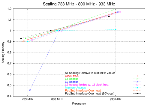
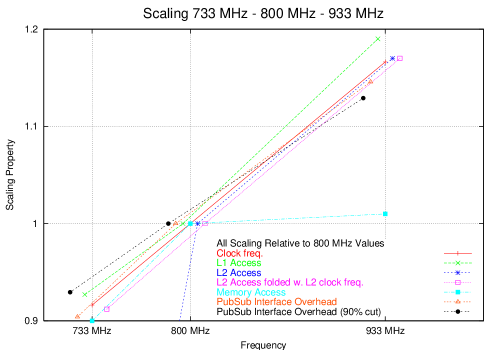
For comparison a scaling plot has been produced, shown in Fig. 8.56, in which the relative values of various measurements are plotted as determined for the three different PCs over their clock frequencies. All values are scaled relative to the values of the 800 MHz PC. The red reference curve shows the clock frequencies. For clarity the curves have been offset slightly to prevent overlapping.
The green curve for the level 1 cache access times shows a perfect scaling, which can be expected as this cache works with the CPU’s core frequency. In the blue level 2 access curve one can see the influence of the level 2 frequency for the 733 MHz CPUs, which is only half the CPU’s frequency unlike for the other CPUs. Folding in this factor of 2 for the 733 MHz PC the pink curve again shows the same perfect scaling property. The cyan memory access curve shows the influence of the chipset (733 MHz to 800 MHz transition) and that for identical motherboards the CPU frequency basically has no influence on the memory access time (800 MHz to 933 MHz transition).
The orange curve shows the scaling behavior of the sum of the times measured in the previous section 8.5.1 without the 90 % cut-off, while the black curve shows the same sum using 90 % cut-off. One can see, as also shown in Table 8.14, that both values somewhat under-scale compared to the theoretical values of 1.091 and 1.166 for 733 MHz to 800 MHz and 800 MHz to 933 MHz respectively. But even taking into account this scaling behavior, the results indicate that the framework can utilize and profit from more than 90 % of CPU performance increases.
Based on those measurements it is assumed that the processing overhead for a complete event announce and release loop is going to drop to or less during the next four to five years, before ALICE (and its HLT) starts to operate. The value of per event announcement is a useful metric that can be used to calculate the overhead in a more complex chain of multiple processes. Even given all scaling uncertainties, however, the existing framework is fast enough to fulfill all ALICE HLT requirements to operate at full speed, already to date. On the other hand, scaling uncertainties are minimized for CPU bound processes, and the interface’s architecture is optimized for smalls amounts of data exchange, making it CPU bound as much as possible.
8.5.3 Future Optimization Options
Preliminary tests with two optimizations of the low-level pipe communication and the pipe proxy classes used in the publisher-subscriber interface show very promising results. The optimizations in question are the replacing of multiple write calls with one writev call that allows to specify multiple blocks to be written with one system call as well as the reduction of new and delete allocation and release calls in the communication functions. Measurements of the interface with these optimizations in place are currently very preliminary and by far not as exhaustive as the ones presented above, but the performances measured so far indicate that a factor of 4 improvement of the maximum performance, and by deduction also overhead, in favour of the new optimized version could be possible.
8.6 Framework System Tests
8.6.1 ALICE HLT Proton-Proton Performance Test
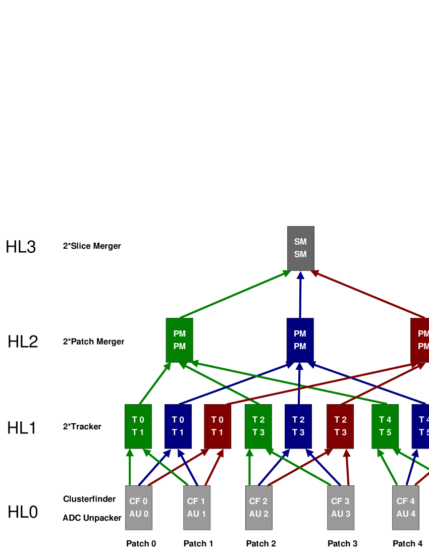
In a large-scale test of the framework in an ALICE High Level Trigger configuration, a setup with 19 nodes has been used to simulate the readout and online data processing of one slice of the ALICE Time Projection Chamber. A slice is one of 18 sectors in one readout plane and therefore represents of the total data volume of the TPC, as described in section 2.2.2. For the test simulated piled-up proton-proton events have been used as the processing power available for the test would not have been sufficient to enable the intended operation at the maximum readout frequency of the TPC of 200 Hz using simulated Pb-Pb events. The limit in this case is the time required to reconstruct the tracks in the event. A schematic view of the cluster configuration used for this test is shown in Figure 8.57.
The data sources for the HLT are the FEPs (see section 2.2.2) connected via optical fibers with the readout electronics mounted on the detectors. Data from each TPC slice is shipped to the HLT over six fibers, the sub-sectors associated with each fiber are called patches. In the present test setup these FEPs are replaced by software in the form of MultFilePublisher components. For each patch the zero-suppressed and run-length encoded simulated ADC data is read from files by the MultFilePublishers and published into the start of the chain. This type of data is similar to the data shipped from the detector. On average the size of the encoded ADC data files is about 14 kB per patch. Encoded ADC data is expanded to sequences of ADC values by the ADCUnpacker components, increasing the size of the data by a factor of about 2 to 3. These values in turn form the input for the ClusterFinder, which reconstructs the three-dimensional coordinates of deposited charges in the detector, called space points. Together with each space point the amount of charge associated with that respective cluster is stored. The MultFilePublisher, ADCUnpacker, and ClusterFinder components run on one node for each patch, called Hierarchy-Level (HL) 0. From this node, the space point data are shipped via bridge components to the next Hierarchy-Level, responsible for combining the space points into track segments, performed by the Tracker component. Since tracking is the most time consuming process in the chain, data is distributed to three trackers on separate nodes using an EventScatterer. Due to the usage of two-processor machines it is possible to run two trackers in parallel on each node, each processing data belonging to the same event but from different patches. At the output of each Hierarchy-Level 1 node the data stream is merged by an EventMerger component and forwarded to Hierarchy-Level 2. On this level the data streams of the six patches are merged into a data stream consisting of events with six blocks of track segments per event. For load balancing reasons this data stream is processed by six PatchMerger components running on three nodes. Each PatchMerger combines the track segments of tracks crossing boundaries between the patches. Since Hierarchy-Level 2 contains three nodes running PatchMerger components the data streams of these nodes are merged in Hierarchy-Level 3 using a SliceMerger component. Again, for load balancing reasons two SliceMerger processes are running on each node. The output obtained from running the processing chain described are reconstructed tracks of one TPC slice.
Operation at a sustained rate of more than 430 events/s has been achieved by using the described setup consisting of 19 nodes with twin CPUs operating at 733 MHz and 800 MHz and connected via Fast Ethernet. The bottlenecks in this setup were the nodes in HL0, especially the ADCUnpacker components. In the final setup of the HLT, these steps will be performed by FPGAs implemented on the RORC cards and thus will not consume time on the FEP CPUs. The maximum TPC readout rate intended for p-p mode in ALICE is 1 kHz and CPUs with more than 3 times the clock frequency relative to those used in the test are already available today. Therefore the use of the framework with these software-only analysis components for online tracking in p-p mode seems to be a practicable option for the ALICE High Level Trigger. Given the necessary increases in CPU processing power and an adequate number of CPUs and thus financial resources, the use in Pb-Pb mode is possible as well.
8.6.2 Framework Fault Tolerance Test
Fault Tolerance Test Setup
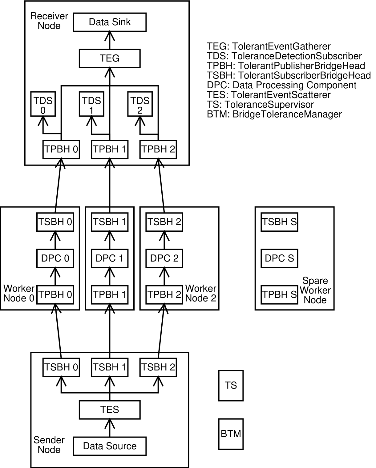
In order to demonstrate the fault tolerance capabilities of the framework described in section 7.5 a test setup has been created using seven computers. The setup used is the sample setup shown in Fig. 7.16 and detailed in section 7.5.1. It is briefly described and shown again here for convenience. Two of the seven computers function as a data source and sink, one supervisor hosts two control programs, three perform identical worker tasks, and one acts as a spare worker node, as displayed in Fig. 8.58.
On the data source computer one process publishes data from a file to a TolerantEventScatterer component (see section 7.5.6) with three output publishers. Each of these publishers in turn supplies its data to one TolerantSubscriberBridgeHead (section 7.5.8) that sends the received data to a TolerantPublisherBridgeHead (section 7.5.8) on one of the worker nodes. Attached to this TolerantPublisherBridgeHead is a dummy processing component (section 7.3.7) that publishes any received data unchanged to a further TolerantSubscriberBridgeHead. This TolerantSubscriberBridgeHead on the worker node in turn sends its input data to a TolerantPublisherBridgeHead on the data sink computer.
Each of the three TolerantPublisherBridgeHead processes on the sink node has two subscribers attached. The first one is an instance of the ToleranceDetectionSubscriber (section 7.5.3), controlling each of the three data streams for continuous operation and the second is one of three subscribers belonging to a TolerantEventGatherer component (section 7.5.7). These gatherer-subscribers merge the three parts of the data stream into one stream again. Attached to the gatherers output publisher is one subscriber process checking for lost events in the data stream, an instance of the EventSupervisor component (section 7.3.5).
Normal Setup Operation
During normal operation the flow of data is basically the one outlined above. Data is published from a file, split up by the scatterer components, and distributed evenly to the three worker nodes, which send their data to the data sink node for data collection and merging into one data stream. This data stream is then checked for lost data.
Node Failure Scenario
If during normal operation of the setup described above one of the three worker nodes fails, the following sequence of events should take place. Due to the node’s failure no more events arrive at the corresponding TolerantPublisherBridgeHead on the data sink node. This causes the timeout of the fault detection component attached to that TolerantPublisherBridgeHead to expire after the specified interval, resulting in a message being sent to one of the control programs. In this supervisor the status of all configured fault detection programs is now checked to determine which of the three data streams is broken. It subsequently sends messages to the scatterer and gatherer components, informing them about the broken link. Now the scatterer marks the output publisher concerned as bad and checks for events that have been sent to that publisher’s path and have not been received back. These events are presumed to be lost and are distributed evenly to the remaining output publishers. All new events arriving after this are also distributed to the remaining publishers. The publisher associated with the broken path does not receive any new events until further notice.
No special action is taken by the Gatherer component upon receiving the notification other than marking the path concerned as broken. EventDone messages for events received from that path are now processed by just marking the event as already done, as the gatherer expects the scatterer to send these events again. Any new event received is first checked against the backlog of EventDone messages that have already been received as well as the list of events marked as done. An event is entered internally into this last list when event done data is received and it belongs to the broken path. If such an event is found, the EventDone message is sent back immediately and the event is removed from the internal tables. An event that cannot be found in these two tables is presumed to be a new event and is handled as usual.
After notifying the scatterer and gatherer components about the failure of the broken data stream, the first control program also informs the second supervisor program of the failure. This program now sends disconnect messages to the corresponding bridge head components on the data source and sink nodes and checks whether a spare node is available. If there is an available spare node it waits for the bridge heads on the sink and source nodes to be properly disconnected and then sends connect commands to them with the addresses of the corresponding bridge head components on the spare node. After it detects that this new connection has been properly established it sends a message to the scatterer and gatherer components to reintegrate the broken path. From this point on the system functions as before with the role of the broken node taken over by the spare. As soon as the functioning node is available again it can be reintegrated into the system as a new spare node.
Fault Tolerance Test Results
To test the fault-tolerance functionality of the system described above, the test setup has been activated with communication between the computers being done via Fast Ethernet. When the data flow chain had been running for a time the network cable was unplugged from one of the worker nodes. This caused the corresponding TolerantSubscriberBridgeHead, that was trying to send from the data source to that node, to block in the TCP code until the specified sending timeout expired. The TolerantPublisherBridgeHead on the data sink did not block while trying to send its accumulated event done messages back to the node. This was presumably because the messages were small enough that they could be placed in buffers of the kernel’s network code or the network interface hardware.
After the timeout in the fault detector component for the broken node’s data path expired, but before the TCP network timeout expired, the first control program was informed of the failure. It subsequently notified the gatherer and scatterer components on the data source and sink, causing lost events to be resent along the remaining two nodes. At the same time, the second control program was notified as well, which then sent disconnect commands to the appropriate bridge head components on the source and sink, and waited for them to become disconnected. Because of mutex semaphores regulating access to the communication classes, the disconnection only happened after the network send timeout expired. When the bridge heads had disconnected from their partners on the ”broken” node, commands were sent to them to clear all events from their internal data structures and to reconnect them to the BridgeHeads on the spare node. As soon as the second control program had determined that the new connection was properly established, it sent commands to the scatterer and gatherer to reactivate the broken path and send new events again to all three data streams.
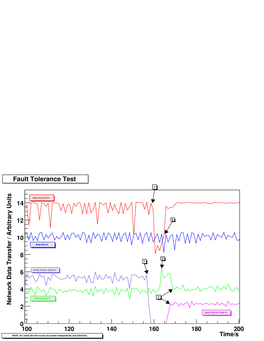
Fig. 8.59 shows results of measurements that were made on the different nodes during the test. In the curves the amount of network traffic going in or coming out of the corresponding nodes is displayed. The measurements were made locally on each of the nodes. Note that the five curves shown are scaled independently to arbitrary values for a better visualization. Real values of the plateaus for the data source and sink node are between 11 MB/s and 12 MB/s and the four other nodes’ (two normal worker/one faulty worker/one spare worker) plateaus are at about 4 MB/s with the peak in the worker node’s curve going to about 6 MB/s. This shows that the network load going out from the data source is evenly distributed to the three active nodes at first and after recovery as well as to the two remaining nodes during the recovery process.
At the points marked 1 the cable is unplugged from the faulty node, causing its incoming network traffic to fall to zero immediately. At the same time or shortly afterwards the network traffic going out of the data source decreases to about two thirds as the TolerantSubscriberBridgeHead sending to the unplugged node blocks. The reason for the decrease to somewhat less than two thirds of the previous might be due to buffers filling up on the source as they do not get freed by the “faulty” node. At point 2 the faulty node has been taken out of the path, and events are passed only to the two remaining worker nodes. The amount of data leaving the data source increases to its previous value, and the amount of data going into the worker node increases by about a factor 1.5, as expected. Finally, at point 3 the spare node has been connected into the chain and the third path has been activated again. Data starts to go into the spare node at the same rate as for the faulty node before the cable was unplugged, and the amount of data going into the regular worker node decreases back to the value before the simulated failure. At this point the data flow chain has fully recovered. During the running time of the test, including some time after the recovery, the event supervisor component has issued no warning about missing events, so not a single event was lost due to this simulated node failure.
Fault Tolerance Test Summary
The presented framework includes a number of components that make a data flow chain tolerant against faults in components of the chain, even against hardware faults of complete nodes. Failures that occur while spare nodes are available cause no further impact except for a short performance decrease until the spare node is activated. With no spares to activate, the system will continue to run with at most a performance decrease corresponding to the processing power loss due to the failure(s). Even in the case of multiple failures no events will be lost. If no output path is available the scatterer component stores events in a list. As soon as a path becomes available again, all events will be sent via this path. Neither of these cases results in the loss of just one single event in the chain. Every event inserted at the beginning arrives at the end of the chain.
8.6.3 System Tests Summary
In the two system tests described above the framework has been demonstrated to be operational and usable in its current form. It has been shown to handle data rates, including processing, within a factor of 2.4 of the highest requirements for operation in the ALICE High Level Trigger. Furthermore, the fault tolerance test has proven that the current concept to ensure fault tolerance works and can in principle also be used in production systems already, despite its proof-of-concept status.
Chapter 9 Conclusion and Outlook
In this thesis a framework has been presented, that has been developed for data flow oriented applications with a particular emphasis on its use in trigger systems of high-energy and nuclear physics. Design and implementation of the framework have been carried out for the data transport software to be used in the High Level Trigger of the future ALICE heavy-ion experiment. To allow flexible configurations the framework is composed of distinct components, that communicate via a defined interface and can be combined in various configurations. Configuration changes are even possible during the runtime of a system.
A first conclusion to be drawn from the framework’s development and its use in a number of setups is, that the composition into multiple independent modules has been proven to be highly functional and efficient. As requirements for specific tests have evolved the modularity has enabled to add functionality in new as well as in existing components and to provide proof-of-concept implementations and prototypes of new characteristics quite fast and easy. Furthermore it has allowed to vary the configurations of tests in a simple and rapid way and therefore to change test setups and to introduce new ones easily. In the two system tests described in section 8.6 it has been demonstrated that the framework is able to operate in conditions closely approaching the ones expected for the operation of the ALICE High Level Trigger. In addition, the current fault tolerance capability also has been shown to be able to handle failures of complete nodes in a running system. The performance impact caused by such a failure is only temporary provided that enough spare nodes are available, otherwise it is at most proportional to the amount of processing power lost.
The separation of the network code into an individual communication class library has turned out to be advantageous, too, since it has allowed to implement and test the communication related functionality of the framework without the need to decide upon a network technology at the current stage. For the tests and developments the currently widespread available and comparatively cheap Gigabit Ethernet TCP/IP solution could be used, however, at the obvious processing overhead. Once the decisions for a network technology and protocol have been made, the appropriate classes have to be implemented only in the communication class library used.
Concerning the performance the framework already meets the requirements set by the conditions of the ALICE High Level Trigger in the existing implementation and with the tested hardware. As the available CPU power does not yet reach the projected level a correspondingly, and quite considerably, larger number of nodes and CPUs would be required to perform the necessary analysis steps of the HLT would it be built today. However, in principle it could be realized at the moment and will be able to operate at the start of the LHC and ALICE. With the potential optimizations discussed in section 8.4.9 and 8.5.3 it should be possible to further enhance the performance and particularly the efficiency of the framework, reducing the CPU power required for the operation at a given rate.
In addition to these performance improvements a number of further tasks will be useful for a full working trigger system. The first of these is a configuration program that provides a plain manner to graphically connect the functional components for a system. The required framework components should be automatically inserted by this configuration program. A more pressing need exists for a process startup, control, and supervision system that can monitor and control the components in a framework configuration. It also has to react to changes in their state by sending appropriate commands, effectively functioning as a Detector Control System (DCS). For this task the framework components have to be modified using the monitoring and control classes described in section 7.5.2 so that they can react as finite state machines (FSM), shifting between states as a result of received commands or other external stimuli. Supervising processes can monitor the states of a number of components, e.g. all components on one node, and react to changes by sending commands. A summary status can be derived from the supervised components’ states and is reported to a further supervisor component that controls multiple nodes. This component in turn can send commands to its subordinate supervisors, which translate them into appropriate commands for the actual framework components. Furthermore, for the use in the ALICE HLT such a system requires an interface to the global ALICE DCS, translating and forwarding its commands and providing it with status information. A final item needed for the framework is a good packaging and distribution mechanism that allows an easy installation of the framework by users not involved in its development. With these enhancements in place, the framework will provide a toolbox from which cluster applications, in particular trigger related ones, can be constructed easily.
Appendix A Benchmark Supplement
A.1 Microbenchmark Programs
A.1.1 Logging Overhead
#include <sys/time.h>
#include <stdio.h>
#define COUNT 1000000000
void test_function1( int* a )
{
(*a)++;
}
void test_function2( unsigned long flags, int* a )
{
if ( flags & 1 )
(*a)++;
}
unsigned long long calc_tdiff( struct timeval* start, struct timeval* stop )
{
unsigned long long tmp;
tmp = (stop->tv_sec - start->tv_sec);
tmp *= 1000000;
tmp += (stop->tv_usec - start->tv_usec);
return tmp;
}
int main( int argc, char** argv )
{
struct timeval start, stop;
unsigned long i;
int n;
int *p = &n;
unsigned long flags = 1;
unsigned long long loopoverhead;
unsigned long long loop_if;
unsigned long long loop_iffunc;
unsigned long long loop_func;
unsigned long long loop_funcif;
gettimeofday( &start, NULL );
for ( i = 0; i < COUNT; i++ )
{
(*p)++;
}
gettimeofday( &stop, NULL );
loopoverhead = calc_tdiff( &start, &stop );
printf( "Loop overhead: %Lu us\n", loopoverhead );
gettimeofday( &start, NULL );
for ( i = 0; i < COUNT; i++ )
{
if ( flags & 1 )
(*p)++;
}
gettimeofday( &stop, NULL );
loop_if = calc_tdiff( &start, &stop );
printf( "Loop with if: %Lu us\n", loop_if );
gettimeofday( &start, NULL );
for ( i = 0; i < COUNT; i++ )
{
test_function1( &n );
}
gettimeofday( &stop, NULL );
loop_func = calc_tdiff( &start, &stop );
printf( "Loop with func: %Lu us\n", loop_func );
gettimeofday( &start, NULL );
for ( i = 0; i < COUNT; i++ )
{
if ( flags & 1 )
test_function1( &n );
}
gettimeofday( &stop, NULL );
loop_iffunc = calc_tdiff( &start, &stop );
printf( "Loop with if and func: %Lu us\n", loop_iffunc );
gettimeofday( &start, NULL );
for ( i = 0; i < COUNT; i++ )
{
test_function2( flags, &n );
}
gettimeofday( &stop, NULL );
loop_funcif = calc_tdiff( &start, &stop );
printf( "Loop with func with if: %Lu us\n", loop_funcif );
return 0;
}
A.2 Minimal Benchmark Process List
PID TTY STAT TIME COMMAND
1 ? S 0:05 init [3]
2 ? SW 0:00 [keventd]
3 ? SWN 0:00 [ksoftirqd_CPU0]
4 ? SW 0:00 [kswapd]
5 ? SW 0:00 [bdflush]
6 ? SW 0:00 [kupdated]
34 ? SW 0:00 [kreiserfsd]
229 ? S 0:00 /sbin/syslogd
233 ? S 0:00 /sbin/klogd -c 1
264 ? SW 0:00 [khubd]
508 tty1 S 0:00 login -- root
509 tty2 S 0:00 /sbin/mingetty tty2
510 tty3 S 0:00 /sbin/mingetty tty3
511 tty4 S 0:00 /sbin/mingetty tty4
512 tty5 S 0:00 /sbin/mingetty tty5
513 tty6 S 0:00 /sbin/mingetty tty6
965 tty1 S 0:00 -bash
1259 tty1 R 0:00 ps x
Appendix B Benchmark Result Tables
The following tables were generated automatically. Layout and number formats may therefore not be optimal. Errors are given as standard deviations where present.
B.1 Micro-Benchmarks
B.1.1 Cache and Memory Reference Tests
| Stride / | Access Time | Access Time | Access Time | Access Time | Access Time | Access Time | Access Time | Access Time |
|---|---|---|---|---|---|---|---|---|
| B | 16B / | 32B / | 64B / | 128B / | 256B / | 512B / | 1kB / | 2kB / |
| ns | ns | ns | ns | ns | ns | ns | ns | |
| 4 | 3.119937 | 4.284117 | 4.107164 | 4.149105 | 4.125885 | 4.121354 | 4.116948 | 4.112793 |
| 8 | 2.095478 | 3.119937 | 4.293430 | 4.111821 | 4.153762 | 4.135198 | 4.116697 | 4.116948 |
| 16 | 1.415612 | 2.114104 | 3.119937 | 4.284117 | 4.107164 | 4.153762 | 4.130542 | 4.116697 |
| 32 | - | 1.396985 | 2.086165 | 3.119937 | 4.274803 | 4.107164 | 4.158419 | 4.125885 |
| 64 | - | - | 1.396985 | 2.095478 | 3.119937 | 4.284117 | 4.107164 | 4.153762 |
| 128 | - | - | - | 1.396985 | 2.095478 | 3.115280 | 4.274803 | 4.107164 |
| 256 | - | - | - | - | 1.406298 | 2.114104 | 3.119937 | 4.274803 |
| 512 | - | - | - | - | - | 1.396985 | 2.095478 | 3.119937 |
| 1024 | - | - | - | - | - | - | 1.415612 | 2.104791 |
| 2048 | - | - | - | - | - | - | - | 1.396985 |
| Stride / | Access Time | Access Time | Access Time | Access Time | Access Time | Access Time | Access Time | Access Time |
|---|---|---|---|---|---|---|---|---|
| B | 4kB / | 8kB / | 16kB / | 32kB / | 64kB / | 128kB / | 256kB / | 512kB / |
| ns | ns | ns | ns | ns | ns | ns | ns | |
| 4 | 4.123116 | 4.120470 | 4.119836 | 4.127914 | 4.125392 | 4.120289 | 13.103088 | 21.351235 |
| 8 | 4.117451 | 4.109139 | 4.106486 | 4.227147 | 4.226086 | 4.223951 | 16.996937 | 28.737954 |
| 16 | 4.112291 | 4.117451 | 4.109139 | 5.919679 | 6.121432 | 6.067987 | 23.380403 | 57.773931 |
| 32 | 4.121354 | 4.112291 | 4.103478 | 13.675857 | 13.689239 | 13.697381 | 39.531339 | 103.797231 |
| 64 | 4.135198 | 4.121354 | 4.093662 | 13.650541 | 13.675857 | 13.689239 | 39.471520 | 103.155772 |
| 128 | 4.149105 | 4.135198 | 4.088756 | 13.609946 | 13.659859 | 13.675857 | 38.860351 | 102.135443 |
| 256 | 4.111821 | 4.149105 | 4.070004 | 13.571027 | 13.628577 | 13.659859 | 38.109574 | 100.362869 |
| 512 | 4.284117 | 4.111821 | 4.028032 | 13.355981 | 13.515140 | 13.609946 | 38.370927 | 97.920575 |
| 1024 | 3.119937 | 4.284117 | 4.195640 | 12.983033 | 13.365295 | 13.515140 | 42.136930 | 98.134957 |
| 2048 | 2.114104 | 3.064057 | 5.224760 | 14.324178 | 13.970265 | 13.905495 | 52.626796 | 111.006944 |
| 4096 | 1.396985 | 8.791702 | 10.952395 | 17.807159 | 20.992651 | 22.520754 | 70.127084 | 138.716264 |
| 8192 | - | 1.396985 | 8.791702 | 10.952395 | 17.807159 | 20.992651 | 22.353106 | 90.046982 |
| 16384 | - | - | 1.396985 | 8.791702 | 10.952395 | 17.807159 | 21.570089 | 22.464872 |
| 32768 | - | - | - | 1.396985 | 8.791702 | 10.952395 | 17.881666 | 22.408305 |
| 65536 | - | - | - | - | 1.396985 | 8.791702 | 10.971022 | 17.639519 |
| 131072 | - | - | - | - | - | 1.396985 | 8.791702 | 10.961709 |
| 262144 | - | - | - | - | - | - | 1.396985 | 8.801015 |
| 524288 | - | - | - | - | - | - | - | 1.396985 |
| Stride / | Access Time | Access Time | Access Time | Access Time | Access Time | Access Time |
|---|---|---|---|---|---|---|
| B | 1MB / | 2MB / | 4MB / | 8MB / | 16MB / | 32MB / |
| ns | ns | ns | ns | ns | ns | |
| 4 | 22.190313 | 22.165477 | 22.156164 | 22.095628 | 22.114255 | 22.129389 |
| 8 | 29.951334 | 29.976169 | 29.914081 | 29.765069 | 29.755756 | 29.758085 |
| 16 | 67.502260 | 68.073471 | 68.470836 | 68.414956 | 68.144873 | 68.014488 |
| 32 | 125.269095 | 127.355258 | 128.522515 | 132.583082 | 134.017318 | 134.753063 |
| 64 | 124.573708 | 126.659870 | 127.851963 | 131.726265 | 133.253634 | 133.961439 |
| 128 | 123.500824 | 125.510352 | 126.163165 | 130.236149 | 131.726265 | 132.508576 |
| 256 | 121.362748 | 123.500824 | 123.722213 | 127.653281 | 129.044056 | 129.789114 |
| 512 | 118.149651 | 120.747474 | 119.606654 | 122.870718 | 124.176343 | 124.921401 |
| 1024 | 117.820079 | 120.723058 | 118.286379 | 119.050344 | 118.953841 | 119.109948 |
| 2048 | 129.101323 | 131.186538 | 129.881359 | 123.670024 | 121.116638 | 122.444970 |
| 4096 | 154.831830 | 155.891959 | 155.312674 | 144.564916 | 138.744231 | 135.103861 |
| 8192 | 139.163736 | 155.131022 | 158.445103 | 158.642966 | 158.125354 | 149.896068 |
| 16384 | 74.616746 | 139.163736 | 160.067689 | 163.701576 | 164.243910 | 164.739547 |
| 32768 | 22.651148 | 79.611073 | 143.116404 | 166.201124 | 176.467295 | 169.239347 |
| 65536 | 23.246521 | 23.508017 | 98.246624 | 149.303220 | 175.176882 | 179.170624 |
| 131072 | 17.639519 | 23.265148 | 23.470761 | 108.458906 | 154.827439 | 184.601428 |
| 262144 | 10.971022 | 17.639519 | 23.246521 | 119.014828 | 140.959307 | 168.264729 |
| 524288 | 8.791702 | 10.971022 | 17.639519 | 23.749450 | 25.426658 | 82.816388 |
| 1048576 | 1.396985 | 8.791702 | 10.961709 | 24.326517 | 25.276866 | 28.090403 |
| 2097152 | - | 1.396985 | 8.782389 | 10.971022 | 25.630388 | 28.108173 |
| 4194304 | - | - | 1.396985 | 8.791702 | 10.971022 | 31.367902 |
| 8388608 | - | - | - | 1.396985 | 8.791702 | 10.971022 |
| 16777216 | - | - | - | - | 1.396985 | 8.791702 |
| 33554432 | - | - | - | - | - | 1.396985 |
| Stride / | Access Time | Access Time | Access Time | Access Time | Access Time | Access Time | Access Time | Access Time |
|---|---|---|---|---|---|---|---|---|
| B | 16B / | 32B / | 64B / | 128B / | 256B / | 512B / | 1kB / | 2kB / |
| ns | ns | ns | ns | ns | ns | ns | ns | |
| 4 | 2.863822 | 3.930211 | 3.767229 | 3.799854 | 3.790599 | 3.776744 | 3.772317 | 3.772778 |
| 8 | 1.969749 | 2.859166 | 3.911585 | 3.767229 | 3.809167 | 3.781285 | 3.776744 | 3.772317 |
| 16 | 1.294540 | 1.969749 | 2.863822 | 3.911585 | 3.767229 | 3.799854 | 3.790599 | 3.776744 |
| 32 | - | 1.294540 | 1.979062 | 2.854509 | 3.930211 | 3.767229 | 3.809167 | 3.790599 |
| 64 | - | - | 1.275913 | 1.974406 | 2.859166 | 3.911585 | 3.767229 | 3.809167 |
| 128 | - | - | - | 1.294540 | 1.965093 | 2.854509 | 3.930211 | 3.767229 |
| 256 | - | - | - | - | 1.275913 | 1.974406 | 2.859166 | 3.930211 |
| 512 | - | - | - | - | - | 1.294540 | 1.974406 | 2.859166 |
| 1024 | - | - | - | - | - | - | 1.275913 | 1.974406 |
| 2048 | - | - | - | - | - | - | - | 1.294540 |
| Stride / | Access Time | Access Time | Access Time | Access Time | Access Time | Access Time | Access Time | Access Time |
|---|---|---|---|---|---|---|---|---|
| B | 4kB / | 8kB / | 16kB / | 32kB / | 64kB / | 128kB / | 256kB / | 512kB / |
| ns | ns | ns | ns | ns | ns | ns | ns | |
| 4 | 3.783017 | 3.770882 | 3.783903 | 3.781973 | 3.782783 | 3.774961 | 11.146069 | 18.232635 |
| 8 | 3.763462 | 3.759722 | 3.766221 | 3.867887 | 3.875471 | 3.871955 | 12.411225 | 23.032938 |
| 16 | 3.772317 | 3.763462 | 3.769040 | 4.707776 | 4.703051 | 4.707598 | 19.400351 | 44.405460 |
| 32 | 3.776744 | 3.772317 | 3.763462 | 6.261545 | 6.269267 | 6.275401 | 32.205430 | 82.680157 |
| 64 | 3.781285 | 3.776744 | 3.758345 | 6.246043 | 6.261545 | 6.269267 | 32.252214 | 82.333883 |
| 128 | 3.799854 | 3.781285 | 3.748802 | 6.203366 | 6.246043 | 6.261545 | 32.350129 | 82.139046 |
| 256 | 3.767229 | 3.799854 | 3.730061 | 6.137790 | 6.208023 | 6.246043 | 32.697405 | 81.440759 |
| 512 | 3.911585 | 3.771885 | 3.692750 | 6.030498 | 6.142447 | 6.212680 | 34.212950 | 80.949678 |
| 1024 | 2.854509 | 3.920898 | 3.869675 | 6.398381 | 6.631421 | 6.631826 | 37.811369 | 83.773744 |
| 2048 | 1.974406 | 2.817256 | 4.833601 | 8.242331 | 8.335591 | 8.428984 | 44.874407 | 91.224267 |
| 4096 | 1.285226 | 8.065269 | 10.030382 | 16.298394 | 18.906425 | 20.248189 | 71.393992 | 108.586495 |
| 8192 | - | 1.294540 | 8.046642 | 10.039696 | 16.335647 | 18.906425 | 20.508975 | 91.090573 |
| 16384 | - | - | 1.275913 | 8.065269 | 10.039696 | 16.298394 | 18.328988 | 19.633478 |
| 32768 | - | - | - | 1.294540 | 8.065269 | 10.039696 | 15.683711 | 19.521117 |
| 65536 | - | - | - | - | 1.294540 | 8.055956 | 10.058322 | 16.168007 |
| 131072 | - | - | - | - | - | 1.285226 | 8.065269 | 10.049009 |
| 262144 | - | - | - | - | - | - | 1.294540 | 8.046642 |
| 524288 | - | - | - | - | - | - | - | 1.275913 |
| Stride / | Access Time | Access Time | Access Time | Access Time | Access Time | Access Time |
|---|---|---|---|---|---|---|
| B | 1MB / | 2MB / | 4MB / | 8MB / | 16MB / | 32MB / |
| ns | ns | ns | ns | ns | ns | |
| 4 | 18.291175 | 18.272549 | 18.328428 | 18.845312 | 19.182917 | 19.352883 |
| 8 | 24.363399 | 24.947027 | 26.803464 | 28.768554 | 29.928051 | 30.521769 |
| 16 | 53.147475 | 54.488579 | 55.581331 | 58.412552 | 60.498714 | 61.551109 |
| 32 | 104.606152 | 109.076500 | 113.770366 | 121.332705 | 126.417726 | 128.941610 |
| 64 | 104.052680 | 108.480453 | 113.149484 | 120.475888 | 125.393271 | 127.870589 |
| 128 | 103.314718 | 107.458660 | 112.056732 | 119.010607 | 123.754144 | 125.989318 |
| 256 | 101.597078 | 105.539958 | 110.183443 | 116.328398 | 120.451053 | 122.562051 |
| 512 | 99.000477 | 102.596898 | 107.367833 | 112.737928 | 116.229057 | 117.967526 |
| 1024 | 102.275938 | 105.206929 | 107.749816 | 110.467275 | 112.823078 | 115.036964 |
| 2048 | 108.980665 | 111.287034 | 112.245953 | 114.748555 | 116.348267 | 117.080552 |
| 4096 | 120.338395 | 119.826373 | 119.622298 | 121.404254 | 122.900932 | 120.083491 |
| 8192 | 121.861492 | 134.074291 | 140.620213 | 146.355216 | 150.317237 | 147.204245 |
| 16384 | 106.595351 | 127.156576 | 138.030827 | 145.482082 | 149.408976 | 157.048625 |
| 32768 | 56.854870 | 101.899192 | 132.675395 | 149.296779 | 160.848062 | 162.578764 |
| 65536 | 20.471095 | 72.809948 | 111.291510 | 137.672163 | 158.122942 | 163.251021 |
| 131072 | 16.168007 | 20.471095 | 89.205228 | 130.821567 | 149.751129 | 156.178194 |
| 262144 | 10.049009 | 16.168007 | 110.654630 | 115.959344 | 133.728713 | 143.116404 |
| 524288 | 8.065269 | 10.049009 | 16.149380 | 21.532835 | 22.148203 | 67.183386 |
| 1048576 | 1.294540 | 8.046642 | 10.058322 | 22.016802 | 21.327938 | 24.756065 |
| 2097152 | - | 1.275913 | 8.065269 | 10.058322 | 20.861944 | 21.812240 |
| 4194304 | - | - | 1.294540 | 8.055956 | 10.049009 | 24.028489 |
| 8388608 | - | - | - | 1.275913 | 8.046642 | 10.049009 |
| 16777216 | - | - | - | - | 1.275913 | 8.065269 |
| 33554432 | - | - | - | - | - | 1.294540 |
| Stride / | Access Time | Access Time | Access Time | Access Time | Access Time | Access Time | Access Time | Access Time |
|---|---|---|---|---|---|---|---|---|
| B | 16B / | 32B / | 64B / | 128B / | 256B / | 512B / | 1kB / | 2kB / |
| ns | ns | ns | ns | ns | ns | ns | ns | |
| 4 | 2.454040 | 3.362087 | 3.222401 | 3.264335 | 3.241101 | 3.236543 | 3.232084 | 3.232479 |
| 8 | 1.699665 | 2.454040 | 3.366744 | 3.231714 | 3.264335 | 3.245758 | 3.231887 | 3.232084 |
| 16 | 1.103618 | 1.699665 | 2.449383 | 3.362087 | 3.231714 | 3.259679 | 3.245758 | 3.236543 |
| 32 | - | 1.108274 | 1.685695 | 2.444726 | 3.362087 | 3.222401 | 3.264335 | 3.241101 |
| 64 | - | - | 1.108274 | 1.695009 | 2.444726 | 3.357431 | 3.231714 | 3.264335 |
| 128 | - | - | - | 1.103618 | 1.685695 | 2.454040 | 3.362087 | 3.231714 |
| 256 | - | - | - | - | 1.098961 | 1.699665 | 2.444726 | 3.362087 |
| 512 | - | - | - | - | - | 1.103618 | 1.690352 | 2.444726 |
| 1024 | - | - | - | - | - | - | 1.103618 | 1.690352 |
| 2048 | - | - | - | - | - | - | - | 1.098961 |
| Stride / | Access Time | Access Time | Access Time | Access Time | Access Time | Access Time | Access Time | Access Time |
|---|---|---|---|---|---|---|---|---|
| B | 4kB / | 8kB / | 16kB / | 32kB / | 64kB / | 128kB / | 256kB / | 512kB / |
| ns | ns | ns | ns | ns | ns | ns | ns | |
| 4 | 3.233268 | 3.239510 | 3.242679 | 3.239688 | 3.238363 | 3.240411 | 10.579824 | 18.083623 |
| 8 | 3.227821 | 3.223950 | 3.225526 | 3.317331 | 3.314486 | 3.318148 | 9.700175 | 24.608203 |
| 16 | 3.232084 | 3.227821 | 3.223950 | 4.036569 | 4.035853 | 4.039091 | 13.765835 | 44.916357 |
| 32 | 3.231887 | 3.232084 | 3.223163 | 5.367039 | 5.374323 | 5.379582 | 20.095280 | 83.616802 |
| 64 | 3.245758 | 3.241200 | 3.213455 | 5.351755 | 5.367039 | 5.374323 | 20.181100 | 83.525976 |
| 128 | 3.264335 | 3.245758 | 3.208602 | 5.323158 | 5.351755 | 5.367039 | 20.345052 | 83.292684 |
| 256 | 3.231714 | 3.264335 | 3.199191 | 5.262294 | 5.318501 | 5.351755 | 21.126406 | 83.030216 |
| 512 | 3.362087 | 3.231714 | 3.157232 | 5.164341 | 5.266951 | 5.323158 | 23.454981 | 83.277545 |
| 1024 | 2.444726 | 3.362087 | 3.301564 | 5.527484 | 5.555509 | 5.634846 | 28.717384 | 85.120108 |
| 2048 | 1.690352 | 2.398160 | 4.121118 | 7.059533 | 7.273851 | 7.255446 | 38.053795 | 91.448222 |
| 4096 | 1.103618 | 6.901113 | 8.605453 | 13.988679 | 16.224134 | 17.342285 | 59.060270 | 109.033967 |
| 8192 | - | 1.103618 | 6.901113 | 8.586827 | 13.988679 | 16.205507 | 16.988361 | 64.575046 |
| 16384 | - | - | 1.103618 | 6.910427 | 8.586827 | 13.988679 | 15.702578 | 16.820712 |
| 32768 | - | - | - | 1.108274 | 6.910427 | 8.586827 | 13.504280 | 16.708437 |
| 65536 | - | - | - | - | 1.108274 | 6.910427 | 8.614767 | 13.839665 |
| 131072 | - | - | - | - | - | 1.108274 | 6.910427 | 8.633393 |
| 262144 | - | - | - | - | - | - | 1.098961 | 6.910427 |
| 524288 | - | - | - | - | - | - | - | 1.108274 |
| Stride / | Access Time | Access Time | Access Time | Access Time | Access Time | Access Time |
|---|---|---|---|---|---|---|
| B | 1MB / | 2MB / | 4MB / | 8MB / | 16MB / | 32MB / |
| ns | ns | ns | ns | ns | ns | |
| 4 | 18.166999 | 18.086284 | 18.095598 | 18.291175 | 18.675346 | 18.971041 |
| 8 | 26.648243 | 26.524067 | 26.300550 | 27.352944 | 29.071234 | 30.100346 |
| 16 | 53.842862 | 54.885944 | 54.948032 | 57.648867 | 60.880557 | 63.255429 |
| 32 | 103.414059 | 105.748574 | 106.245279 | 112.839043 | 120.010227 | 125.002116 |
| 64 | 103.030886 | 105.500221 | 105.996927 | 112.354755 | 119.358301 | 124.201179 |
| 128 | 102.678935 | 105.329922 | 105.798244 | 111.411015 | 118.017197 | 122.599304 |
| 256 | 102.212352 | 105.142593 | 105.244773 | 109.573205 | 115.434329 | 119.432807 |
| 512 | 101.649572 | 104.596538 | 104.427338 | 106.607165 | 111.361345 | 114.689271 |
| 1024 | 103.101956 | 106.569320 | 106.749996 | 107.924143 | 110.524041 | 112.255414 |
| 2048 | 108.756271 | 111.437219 | 111.489069 | 113.056552 | 115.474065 | 116.910253 |
| 4096 | 120.562350 | 122.444302 | 122.400719 | 121.631320 | 121.208929 | 120.083491 |
| 8192 | 108.139023 | 121.831427 | 126.333798 | 133.739682 | 140.856183 | 142.282055 |
| 16384 | 67.891364 | 108.288180 | 122.353989 | 137.104708 | 148.082343 | 151.972617 |
| 32768 | 17.565816 | 70.499704 | 110.450961 | 134.148943 | 148.983452 | 161.216373 |
| 65536 | 17.583907 | 18.571706 | 71.468516 | 118.580032 | 140.792936 | 159.496397 |
| 131072 | 13.858291 | 17.565280 | 18.608961 | 73.349528 | 123.054751 | 152.887083 |
| 262144 | 8.624080 | 13.858291 | 17.583907 | 70.826414 | 124.932733 | 144.831712 |
| 524288 | 6.901113 | 8.614767 | 13.858291 | 18.198598 | 75.939956 | 85.350823 |
| 1048576 | 1.103618 | 6.910427 | 8.614767 | 19.129658 | 18.328988 | 21.235451 |
| 2097152 | - | 1.098961 | 6.891800 | 8.624080 | 17.658145 | 18.682901 |
| 4194304 | - | - | 1.103618 | 6.901113 | 8.633393 | 20.619796 |
| 8388608 | - | - | - | 1.103618 | 6.901113 | 8.614767 |
| 16777216 | - | - | - | - | 1.103618 | 6.910427 |
| 33554432 | - | - | - | - | - | 1.098961 |
B.2 Network Reference Tests
B.2.1 TCP Network Reference Throughput
Plateau Determination
| Block Count | Send Rate | Send Rate | Send Rate | Send Rate |
|---|---|---|---|---|
| FE, NODELAY / | FE, DELAY / | GbE, NODELAY / | GbE, DELAY / | |
| Hz | Hz | Hz | Hz | |
| 1 | 34762.024000 | 36024.591000 | 33636.267000 | 35230.800000 |
| 1171.626428 | 1379.099518 | 1608.692948 | 836.383433 | |
| 2 | 56049.666000 | 64545.192000 | 57497.668000 | 64732.369000 |
| 1246.266239 | 3641.027099 | 1227.956107 | 3753.324588 | |
| 4 | 101077.648000 | 121682.192000 | 92851.441000 | 117885.076000 |
| 2623.648395 | 3546.405800 | 2011.312404 | 7830.057004 | |
| 8 | 176265.897000 | 206891.591000 | 165151.370000 | 194235.170000 |
| 3090.387552 | 6099.068053 | 5639.131963 | 16342.841257 | |
| 16 | 245919.277000 | 321384.553000 | 269439.340000 | 297082.766000 |
| 5923.767780 | 5680.180492 | 4606.176882 | 19962.085996 | |
| 32 | 374478.611000 | 453408.809000 | 382678.982000 | 412356.658000 |
| 8697.238639 | 8326.814667 | 21097.064489 | 14941.783034 | |
| 64 | 490861.289000 | 504325.713000 | 504806.114000 | 508059.696000 |
| 5554.282730 | 53088.240184 | 6129.283017 | 7963.608699 | |
| 128 | 459084.126000 | 533575.004000 | 590908.308000 | 528582.354000 |
| 7891.963651 | 11466.115177 | 11493.295303 | 24750.547209 | |
| 256 | 563578.170000 | 583768.424000 | 501443.959000 | 520125.878000 |
| 10467.080730 | 36542.412165 | 36361.652041 | 7845.657579 | |
| 512 | 483018.009000 | 589387.908000 | 470709.769000 | 540798.963000 |
| 45099.331912 | 11086.360004 | 16127.017903 | 8856.601167 | |
| 1024 | 515464.206000 | 578967.730000 | 480516.545000 | 555329.548000 |
| 24385.934142 | 7989.583940 | 24053.138141 | 7664.634060 | |
| 2048 | 541769.991000 | 611026.695000 | 465009.834000 | 578306.314000 |
| 8352.675518 | 7956.362576 | 27368.681707 | 4608.400446 | |
| 4096 | 563640.718000 | 632970.834000 | 475836.800000 | 590152.055000 |
| 16024.710966 | 6731.016121 | 23130.926457 | 5069.882137 | |
| 8192 | 409988.585000 | 567643.520000 | 497967.782000 | 602657.678000 |
| 166519.218525 | 11345.720132 | 18256.745780 | 10454.036587 | |
| 16384 | 366357.583000 | 426957.552000 | 544150.356000 | 603685.001000 |
| 114901.906428 | 3282.740186 | 16151.690602 | 9487.956841 | |
| 32768 | 314569.770000 | 398609.499000 | 566200.256000 | 594467.220000 |
| 99632.085865 | 4497.825895 | 10558.574848 | 5096.971612 | |
| 65536 | 347603.793000 | 382581.572000 | 542876.246000 | 570563.287000 |
| 79699.617030 | 2164.759754 | 35814.834138 | 5171.315639 | |
| 131072 | 356715.221000 | 374648.704000 | 558076.782000 | 560064.224000 |
| 26200.166331 | 702.025526 | 17219.383680 | 3770.692591 | |
| 262144 | 351599.194000 | 371414.588000 | 550963.983000 | 555699.622000 |
| 40710.471890 | 423.872809 | 3670.444944 | 3034.847635 | |
| 524288 | 364280.425000 | 369427.564000 | 548491.034000 | 554689.250000 |
| 8027.007388 | 206.642156 | 5823.155026 | 3458.260106 | |
| 1048576 | 350792.952000 | 368617.328000 | 548318.330000 | 555513.475000 |
| 24333.585832 | 70.546718 | 3490.104039 | 2207.289208 | |
| 2097152 | 360442.981000 | 368097.851000 | 545302.074000 | 553018.943000 |
| 6156.412269 | 67.127455 | 8283.334501 | 867.574849 | |
| 4194304 | 363218.398000 | 367880.837000 | 548698.375000 | 554285.176000 |
| 6547.539011 | 27.387992 | 2412.906486 | 3657.615136 | |
| 8388608 | 364353.439000 | 367765.872000 | 547462.788000 | 555960.339000 |
| 2772.607469 | 11.653661 | 7815.232143 | 3950.269461 |
Plateau Throughput Measurement
| Block Size / | Send Rate | Send Rate | Send Rate | Send Rate |
|---|---|---|---|---|
| B | FE, NODELAY / | FE, DELAY / | GbE, NODELAY / | GbE, DELAY / |
| Hz | Hz | Hz | Hz | |
| 8 | 642587.764937 | 646578.653660 | 684377.610693 | 687405.107604 |
| 7860.841550 | 5965.302372 | 7122.679994 | 5121.024119 | |
| 16 | 540255.800438 | 599165.742889 | 606062.147356 | 623164.961234 |
| 107688.853272 | 4129.651092 | 11968.191890 | 6217.346900 | |
| 32 | 355438.647634 | 366263.323020 | 536517.926126 | 553240.164277 |
| 19813.112091 | 356.680789 | 60838.361852 | 11124.139815 | |
| 64 | 183481.525266 | 183478.828410 | 482040.079291 | 486966.859860 |
| 68.706614 | 53.165798 | 7830.840018 | 7163.113167 | |
| 128 | 91835.492471 | 91817.495635 | 385357.406411 | 380998.612735 |
| 14.750969 | 11.127230 | 7778.389132 | 4549.261135 | |
| 256 | 45933.037158 | 45934.848123 | 263536.262073 | 263417.359516 |
| 1.826990 | 2.857413 | 7619.557017 | 8132.415341 | |
| 512 | 22970.109740 | 22972.348117 | 158099.839484 | 159681.591943 |
| 6.482007 | 0.775053 | 15310.047019 | 8016.824854 | |
| 1024 | 11487.750301 | 11487.586692 | 75959.020887 | 77532.072365 |
| 0.182993 | 0.308084 | 221.155844 | 1939.331411 | |
| 2048 | 5744.183763 | 5744.138262 | 37441.339012 | 38787.852961 |
| 0.013531 | 0.030586 | 385.693773 | 497.476955 | |
| 4096 | 2872.163471 | 2872.187246 | 18597.955221 | 19244.425211 |
| 0.008969 | 0.012934 | 104.212209 | 227.414922 | |
| 8192 | 1436.110593 | 1436.118012 | 9234.940990 | 9601.841017 |
| 0.003387 | 0.002604 | 47.894897 | 48.958558 | |
| 16384 | 718.059826 | 718.066146 | 5059.561268 | 5038.727297 |
| 0.007890 | 0.000726 | 14.164281 | 13.694561 | |
| 32768 | 359.029917 | 359.034180 | 2429.494282 | 2517.646849 |
| 0.006375 | 0.000766 | 5.505879 | 15.397058 | |
| 65536 | 179.516739 | 179.517567 | 1378.442222 | 1414.390266 |
| 0.000051 | 0.000095 | 15.148842 | 13.159668 | |
| 131072 | 89.758451 | 89.758855 | 608.367899 | 622.802220 |
| 0.000026 | 0.000196 | 5.228913 | 2.640861 | |
| 262144 | 44.879254 | 44.879485 | 285.310505 | 289.880436 |
| 0.000012 | 0.000012 | 0.485072 | 0.500977 | |
| 524288 | 22.439631 | 22.439744 | 137.867446 | 138.674233 |
| 0.000003 | 0.000002 | 0.187848 | 0.110837 | |
| 1048576 | 11.219817 | 11.219874 | 68.905818 | 68.999439 |
| 0.000001 | 0.000001 | 0.207060 | 0.094263 | |
| 2097152 | 5.609909 | 5.609938 | 34.290534 | 34.289766 |
| 0.000000 | 0.000000 | 0.036978 | 0.031889 | |
| 4194304 | 2.804955 | 2.804969 | 17.142241 | 17.139225 |
| 0.000000 | 0.000000 | 0.023407 | 0.023292 |
| Block Size / | Network Throughput | Network Throughput | Network Throughput | Network Throughput |
|---|---|---|---|---|
| B | FE, NODELAY / | FE, DELAY / | GbE, NODELAY / | GbE, DELAY / |
| 8 | 5140702.119496 | 5172629.229280 | 5475020.885544 | 5499240.860832 |
| 62886.732400 | 47722.418976 | 56981.439952 | 40968.192952 | |
| 16 | 8644092.807008 | 9586651.886224 | 9696994.357696 | 9970639.379744 |
| 1723021.652352 | 66074.417472 | 191491.070240 | 99477.550400 | |
| 32 | 11374036.724288 | 11720426.336640 | 17168573.636032 | 17703685.256864 |
| 634019.586912 | 11413.785248 | 1946827.579264 | 355972.474080 | |
| 64 | 11742817.617024 | 11742645.018240 | 30850565.074624 | 31165879.031040 |
| 4397.223296 | 3402.611072 | 501173.761152 | 458439.242688 | |
| 128 | 11754943.036288 | 11752639.441280 | 49325748.020608 | 48767822.430080 |
| 1888.124032 | 1424.285440 | 995633.808896 | 582305.425280 | |
| 256 | 11758857.512448 | 11759321.119488 | 67465283.090688 | 67434844.036096 |
| 467.709440 | 731.497728 | 1950606.596352 | 2081898.327296 | |
| 512 | 11760696.186880 | 11761842.235904 | 80947117.815808 | 81756975.074816 |
| 3318.787584 | 396.827136 | 7838744.073728 | 4104614.325248 | |
| 1024 | 11763456.308224 | 11763288.772608 | 77782037.388288 | 79392842.101760 |
| 187.384832 | 315.478016 | 226463.584256 | 1985875.364864 | |
| 2048 | 11764088.346624 | 11763995.160576 | 76679862.296576 | 79437522.864128 |
| 27.711488 | 62.640128 | 789900.847104 | 1018832.803840 | |
| 4096 | 11764381.577216 | 11764478.959616 | 76177224.585216 | 78825165.664256 |
| 36.737024 | 52.977664 | 426853.208064 | 931491.520512 | |
| 8192 | 11764617.977856 | 11764678.754304 | 75652636.590080 | 78658281.611264 |
| 27.746304 | 21.331968 | 392354.996224 | 401068.507136 | |
| 16384 | 11764692.189184 | 11764795.736064 | 82895851.814912 | 82554508.034048 |
| 129.269760 | 11.894784 | 232067.579904 | 224371.687424 | |
| 32768 | 11764692.320256 | 11764832.010240 | 79609668.632576 | 82498251.948032 |
| 208.896000 | 25.100288 | 180416.643072 | 504530.796544 | |
| 65536 | 11764809.007104 | 11764863.270912 | 90337589.460992 | 92693480.472576 |
| 3.342336 | 6.225920 | 992794.509312 | 862432.002048 | |
| 131072 | 11764819.689472 | 11764872.642560 | 79739997.257728 | 81631932.579840 |
| 3.407872 | 25.690112 | 685364.084736 | 346142.932992 | |
| 262144 | 11764827.160576 | 11764887.715840 | 74792437.022720 | 75990417.014784 |
| 3.145728 | 3.145728 | 127158.714368 | 131328.114688 | |
| 524288 | 11764829.257728 | 11764888.502272 | 72282247.528448 | 72705236.271104 |
| 1.572864 | 1.048576 | 98486.452224 | 58110.509056 | |
| 1048576 | 11764830.830592 | 11764890.599424 | 72252987.015168 | 72351155.748864 |
| 1.048576 | 1.048576 | 217118.146560 | 98841.919488 | |
| 2097152 | 11764831.879168 | 11764892.696576 | 71912461.959168 | 71910851.346432 |
| 0.000000 | 0.000000 | 77548.486656 | 66876.080128 | |
| 4194304 | 11764833.976320 | 11764892.696576 | 71899769.995264 | 71887119.974400 |
| 0.000000 | 0.000000 | 98176.073728 | 97693.728768 |
| Block Size / | CPU Usage | CPU Usage | CPU Usage | CPU Usage |
|---|---|---|---|---|
| B | FE, NODELAY / | FE, DELAY / | GbE, NODELAY / | GbE, DELAY / |
| % | % | % | % | |
| 8 | 93.600000 | 91.000000 | 97.000000 | 97.200000 |
| 2.154066 | 1.612452 | 1.341640 | 1.326650 | |
| 16 | 94.400000 | 93.200000 | 96.200000 | 97.200000 |
| 4.543126 | 0.979796 | 2.088062 | 1.326650 | |
| 32 | 61.800000 | 61.800000 | 97.400000 | 101.200000 |
| 3.627672 | 1.400000 | 10.002000 | 2.227106 | |
| 64 | 36.000000 | 36.200000 | 99.200000 | 100.400000 |
| 0.000000 | 0.600000 | 2.039608 | 1.743560 | |
| 128 | 24.200000 | 24.000000 | 100.000000 | 99.000000 |
| 0.600000 | 0.000000 | 2.190890 | 3.255764 | |
| 256 | 18.000000 | 18.000000 | 98.600000 | 96.000000 |
| 0.000000 | 0.000000 | 2.009976 | 4.098780 | |
| 512 | 14.600000 | 14.000000 | 93.600000 | 94.000000 |
| 0.916516 | 0.000000 | 5.122500 | 3.577708 | |
| 1024 | 14.000000 | 14.000000 | 75.000000 | 77.400000 |
| 0.000000 | 0.000000 | 1.341640 | 2.200000 | |
| 2048 | 12.000000 | 12.000000 | 68.400000 | 71.000000 |
| 0.000000 | 0.000000 | 1.200000 | 1.341640 | |
| 4096 | 12.000000 | 12.000000 | 65.600000 | 68.000000 |
| 0.000000 | 0.000000 | 0.800000 | 1.264912 | |
| 8192 | 12.000000 | 12.000000 | 64.000000 | 66.400000 |
| 0.000000 | 0.000000 | 0.000000 | 0.800000 | |
| 16384 | 12.000000 | 12.000000 | 69.200000 | 68.400000 |
| 0.000000 | 0.000000 | 0.979796 | 0.800000 | |
| 32768 | 12.200000 | 12.000000 | 64.800000 | 68.200000 |
| 0.600000 | 0.000000 | 0.979796 | 0.600000 | |
| 65536 | 14.000000 | 13.800000 | 77.800000 | 82.000000 |
| 0.000000 | 0.600000 | 1.077032 | 3.098386 | |
| 131072 | 14.000000 | 14.000000 | 77.400000 | 79.000000 |
| 0.000000 | 0.000000 | 1.280624 | 1.000000 | |
| 262144 | 16.000000 | 14.800000 | 76.000000 | 76.800000 |
| 0.000000 | 0.979796 | 0.000000 | 0.979796 | |
| 524288 | 16.000000 | 16.000000 | 72.000000 | 74.000000 |
| 0.000000 | 0.000000 | 0.000000 | 0.000000 | |
| 1048576 | 16.000000 | 16.000000 | 72.200000 | 72.200000 |
| 0.000000 | 0.000000 | 0.600000 | 0.600000 | |
| 2097152 | 16.000000 | 16.000000 | 72.000000 | 72.000000 |
| 0.000000 | 0.000000 | 0.000000 | 0.000000 | |
| 4194304 | 16.000000 | 15.500000 | 72.000000 | 72.000000 |
| 0.000000 | 0.866026 | 0.000000 | 0.000000 |
| Block Size / | CPU Usage | CPU Usage | CPU Usage | CPU Usage |
|---|---|---|---|---|
| B | FE, NODELAY / | FE, DELAY / | GbE, NODELAY / | GbE, DELAY / |
| % | % | % | % | |
| 8 | 97.584911 | 97.972927 | 100.962679 | 101.611486 |
| 5.452952 | 1.244379 | 0.776517 | 1.579818 | |
| 16 | 102.316781 | 105.639370 | 101.767603 | 96.024573 |
| 37.730304 | 0.745266 | 8.206925 | 5.253103 | |
| 32 | 66.124514 | 65.880738 | 99.890350 | 101.211413 |
| 11.387698 | 4.452355 | 20.700743 | 7.177821 | |
| 64 | 43.824868 | 43.832128 | 107.354256 | 104.890441 |
| 0.036705 | 0.037239 | 7.014128 | 7.251209 | |
| 128 | 29.970971 | 30.338139 | 110.420988 | 110.496897 |
| 0.042477 | 1.190528 | 5.431014 | 1.751433 | |
| 256 | 25.873875 | 25.876750 | 113.319081 | 112.594201 |
| 0.004476 | 0.053481 | 7.045837 | 8.211848 | |
| 512 | 22.183905 | 21.940505 | 110.100883 | 110.267951 |
| 0.746565 | 0.007161 | 14.871812 | 10.484392 | |
| 1024 | 19.971330 | 21.746507 | 91.330686 | 93.878050 |
| 0.000880 | 0.890395 | 2.132443 | 5.184867 | |
| 2048 | 20.040660 | 19.829729 | 84.663808 | 86.833058 |
| 1.055911 | 1.036580 | 2.573642 | 3.202314 | |
| 4096 | 18.493000 | 19.314917 | 79.820877 | 82.368289 |
| 0.001171 | 1.007737 | 1.529543 | 2.743990 | |
| 8192 | 18.246516 | 18.246519 | 77.904986 | 80.775083 |
| 0.000386 | 0.001336 | 1.648082 | 0.788147 | |
| 16384 | 18.123261 | 18.123262 | 83.859847 | 83.215115 |
| 0.000302 | 0.000310 | 0.458268 | 1.401311 | |
| 32768 | 18.262313 | 18.262315 | 79.193265 | 81.715930 |
| 0.606505 | 0.604899 | 1.291466 | 1.601138 | |
| 65536 | 19.433213 | 20.034240 | 94.425162 | 95.470605 |
| 0.918147 | 0.000042 | 3.054885 | 2.372788 | |
| 131072 | 20.017120 | 20.017120 | 88.711720 | 90.534550 |
| 0.000020 | 0.000985 | 2.124094 | 0.765438 | |
| 262144 | 20.008560 | 20.008560 | 86.234002 | 88.243298 |
| 0.000212 | 0.000209 | 0.292433 | 0.295185 | |
| 524288 | 20.004280 | 20.604408 | 84.110444 | 84.111090 |
| 0.000368 | 0.916774 | 0.229076 | 0.134414 | |
| 1048576 | 20.002140 | 21.002247 | 84.055200 | 84.055275 |
| 0.000029 | 1.000401 | 0.505558 | 0.228715 | |
| 2097152 | 20.001070 | 22.001177 | 84.027470 | 84.027469 |
| 0.000002 | 0.000045 | 0.181035 | 0.156655 | |
| 4194304 | 20.000535 | 21.500575 | 84.013732 | 84.013730 |
| 0.000002 | 0.866052 | 0.228966 | 0.228885 |
| Block Size / | CPU Usage / Rate | CPU Usage / Rate | CPU Usage / Rate | CPU Usage / Rate |
|---|---|---|---|---|
| B | FE, NODELAY / | FE, DELAY / | GbE, NODELAY / | GbE, DELAY / |
| 8 | 0.000146 | 0.000141 | 0.000142 | 0.000141 |
| 0.000005 | 0.000004 | 0.000003 | 0.000003 | |
| 16 | 0.000175 | 0.000156 | 0.000159 | 0.000156 |
| 0.000043 | 0.000003 | 0.000007 | 0.000004 | |
| 32 | 0.000174 | 0.000169 | 0.000182 | 0.000183 |
| 0.000020 | 0.000004 | 0.000039 | 0.000008 | |
| 64 | 0.000196 | 0.000197 | 0.000206 | 0.000206 |
| 0.000000 | 0.000003 | 0.000008 | 0.000007 | |
| 128 | 0.000264 | 0.000261 | 0.000259 | 0.000260 |
| 0.000007 | 0.000000 | 0.000011 | 0.000012 | |
| 256 | 0.000392 | 0.000392 | 0.000374 | 0.000364 |
| 0.000000 | 0.000000 | 0.000018 | 0.000027 | |
| 512 | 0.000636 | 0.000609 | 0.000592 | 0.000589 |
| 0.000040 | 0.000000 | 0.000090 | 0.000052 | |
| 1024 | 0.001219 | 0.001219 | 0.000987 | 0.000998 |
| 0.000000 | 0.000000 | 0.000021 | 0.000053 | |
| 2048 | 0.002089 | 0.002089 | 0.001827 | 0.001830 |
| 0.000000 | 0.000000 | 0.000051 | 0.000058 | |
| 4096 | 0.004178 | 0.004178 | 0.003527 | 0.003533 |
| 0.000000 | 0.000000 | 0.000063 | 0.000107 | |
| 8192 | 0.008356 | 0.008356 | 0.006930 | 0.006915 |
| 0.000000 | 0.000000 | 0.000036 | 0.000119 | |
| 16384 | 0.016712 | 0.016712 | 0.013677 | 0.013575 |
| 0.000000 | 0.000000 | 0.000232 | 0.000196 | |
| 32768 | 0.033980 | 0.033423 | 0.026672 | 0.027089 |
| 0.001672 | 0.000000 | 0.000464 | 0.000404 | |
| 65536 | 0.077987 | 0.076873 | 0.056441 | 0.057976 |
| 0.000000 | 0.003342 | 0.001402 | 0.002730 | |
| 131072 | 0.155974 | 0.155973 | 0.127226 | 0.126846 |
| 0.000000 | 0.000000 | 0.003199 | 0.002144 | |
| 262144 | 0.356512 | 0.329772 | 0.266376 | 0.264937 |
| 0.000000 | 0.021832 | 0.000453 | 0.003838 | |
| 524288 | 0.713024 | 0.713021 | 0.522241 | 0.533625 |
| 0.000000 | 0.000000 | 0.000712 | 0.000427 | |
| 1048576 | 1.426048 | 1.426041 | 1.047807 | 1.046385 |
| 0.000000 | 0.000000 | 0.011856 | 0.010125 | |
| 2097152 | 2.852096 | 2.852081 | 2.099705 | 2.099752 |
| 0.000000 | 0.000000 | 0.002264 | 0.001953 | |
| 4194304 | 5.704191 | 5.525908 | 4.200151 | 4.200890 |
| 0.000000 | 0.308747 | 0.005735 | 0.005709 |
| Block Size / | CPU Usage / Rate | CPU Usage / Rate | CPU Usage / Rate | CPU Usage / Rate |
|---|---|---|---|---|
| B | FE, NODELAY / | FE, DELAY / | GbE, NODELAY / | GbE, DELAY / |
| 8 | 0.000152 | 0.000152 | 0.000148 | 0.000148 |
| 0.000010 | 0.000003 | 0.000003 | 0.000003 | |
| 16 | 0.000189 | 0.000176 | 0.000168 | 0.000154 |
| 0.000108 | 0.000002 | 0.000017 | 0.000010 | |
| 32 | 0.000186 | 0.000180 | 0.000186 | 0.000183 |
| 0.000042 | 0.000012 | 0.000060 | 0.000017 | |
| 64 | 0.000239 | 0.000239 | 0.000223 | 0.000215 |
| 0.000000 | 0.000000 | 0.000018 | 0.000018 | |
| 128 | 0.000326 | 0.000330 | 0.000287 | 0.000290 |
| 0.000001 | 0.000013 | 0.000020 | 0.000008 | |
| 256 | 0.000563 | 0.000563 | 0.000430 | 0.000427 |
| 0.000000 | 0.000001 | 0.000039 | 0.000044 | |
| 512 | 0.000966 | 0.000955 | 0.000696 | 0.000691 |
| 0.000033 | 0.000000 | 0.000162 | 0.000100 | |
| 1024 | 0.001738 | 0.001893 | 0.001202 | 0.001211 |
| 0.000000 | 0.000078 | 0.000032 | 0.000097 | |
| 2048 | 0.003489 | 0.003452 | 0.002261 | 0.002239 |
| 0.000184 | 0.000180 | 0.000092 | 0.000111 | |
| 4096 | 0.006439 | 0.006725 | 0.004292 | 0.004280 |
| 0.000000 | 0.000351 | 0.000106 | 0.000193 | |
| 8192 | 0.012706 | 0.012705 | 0.008436 | 0.008412 |
| 0.000000 | 0.000001 | 0.000222 | 0.000125 | |
| 16384 | 0.025239 | 0.025239 | 0.016575 | 0.016515 |
| 0.000001 | 0.000000 | 0.000137 | 0.000323 | |
| 32768 | 0.050866 | 0.050865 | 0.032597 | 0.032457 |
| 0.001690 | 0.001685 | 0.000605 | 0.000834 | |
| 65536 | 0.108253 | 0.111600 | 0.068501 | 0.067499 |
| 0.005115 | 0.000000 | 0.002969 | 0.002306 | |
| 131072 | 0.223011 | 0.223010 | 0.145819 | 0.145366 |
| 0.000000 | 0.000011 | 0.004745 | 0.001845 | |
| 262144 | 0.445831 | 0.445829 | 0.302246 | 0.304413 |
| 0.000005 | 0.000005 | 0.001539 | 0.001544 | |
| 524288 | 0.891471 | 0.918210 | 0.610082 | 0.606537 |
| 0.000017 | 0.040855 | 0.002493 | 0.001454 | |
| 1048576 | 1.782751 | 1.871879 | 1.219856 | 1.218202 |
| 0.000003 | 0.089163 | 0.011003 | 0.004979 | |
| 2097152 | 3.565311 | 3.921822 | 2.450457 | 2.450512 |
| 0.000000 | 0.000008 | 0.007922 | 0.006848 | |
| 4194304 | 7.130430 | 7.665174 | 4.900977 | 4.901839 |
| 0.000001 | 0.308756 | 0.020049 | 0.020016 |
| Block Size / | CPU Usage / Throughput | CPU Usage / Throughput | CPU Usage / Throughput | CPU Usage / Throughput |
|---|---|---|---|---|
| B | FE, NODELAY / | FE, DELAY / | GbE, NODELAY / | GbE, DELAY / |
| 8 | 19.092082 | 18.447177 | 18.577439 | 18.533755 |
| 0.672930 | 0.497064 | 0.450297 | 0.391032 | |
| 16 | 11.451240 | 10.194099 | 10.402503 | 10.222171 |
| 2.833674 | 0.177429 | 0.431214 | 0.241506 | |
| 32 | 5.697361 | 5.528979 | 5.948735 | 5.994000 |
| 0.652022 | 0.130636 | 1.285431 | 0.252433 | |
| 64 | 3.214623 | 3.232530 | 3.371696 | 3.377958 |
| 0.001204 | 0.054515 | 0.124098 | 0.108351 | |
| 128 | 2.158712 | 2.141291 | 2.125819 | 2.128638 |
| 0.053869 | 0.000259 | 0.089484 | 0.095420 | |
| 256 | 1.605119 | 1.605056 | 1.532486 | 1.492749 |
| 0.000064 | 0.000100 | 0.075548 | 0.109819 | |
| 512 | 1.301726 | 1.248109 | 1.212479 | 1.205599 |
| 0.082083 | 0.000042 | 0.183770 | 0.106413 | |
| 1024 | 1.247938 | 1.247956 | 1.011071 | 1.022256 |
| 0.000020 | 0.000033 | 0.021030 | 0.054626 | |
| 2048 | 1.069604 | 1.069612 | 0.935351 | 0.937201 |
| 0.000002 | 0.000006 | 0.026045 | 0.029730 | |
| 4096 | 1.069577 | 1.069568 | 0.902981 | 0.904574 |
| 0.000003 | 0.000005 | 0.016072 | 0.027516 | |
| 8192 | 1.069556 | 1.069550 | 0.887066 | 0.885164 |
| 0.000002 | 0.000002 | 0.004601 | 0.015178 | |
| 16384 | 1.069549 | 1.069539 | 0.875333 | 0.868791 |
| 0.000012 | 0.000001 | 0.014844 | 0.012523 | |
| 32768 | 1.087375 | 1.069536 | 0.853511 | 0.866841 |
| 0.053497 | 0.000002 | 0.014840 | 0.012927 | |
| 65536 | 1.247795 | 1.229963 | 0.903048 | 0.927608 |
| 0.000000 | 0.053477 | 0.022426 | 0.043680 | |
| 131072 | 1.247793 | 1.247788 | 1.017805 | 1.014768 |
| 0.000000 | 0.000003 | 0.025588 | 0.017148 | |
| 262144 | 1.426049 | 1.319088 | 1.065506 | 1.059747 |
| 0.000000 | 0.087327 | 0.001812 | 0.015351 | |
| 524288 | 1.426048 | 1.426041 | 1.044482 | 1.067249 |
| 0.000000 | 0.000000 | 0.001423 | 0.000853 | |
| 1048576 | 1.426048 | 1.426041 | 1.047807 | 1.046385 |
| 0.000000 | 0.000000 | 0.011856 | 0.010125 | |
| 2097152 | 1.426048 | 1.426041 | 1.049852 | 1.049876 |
| 0.000000 | 0.000000 | 0.001132 | 0.000976 | |
| 4194304 | 1.426048 | 1.381477 | 1.050038 | 1.050223 |
| 0.000000 | 0.077187 | 0.001434 | 0.001427 |
| Block Size / | CPU Usage / Throughput | CPU Usage / Throughput | CPU Usage / Throughput | CPU Usage / Throughput |
|---|---|---|---|---|
| B | FE, NODELAY / | FE, DELAY / | GbE, NODELAY / | GbE, DELAY / |
| 8 | 19.904905 | 19.860703 | 19.336372 | 19.374922 |
| 1.355764 | 0.435491 | 0.349963 | 0.445572 | |
| 16 | 12.411589 | 11.554702 | 11.004551 | 10.098556 |
| 7.050887 | 0.161155 | 1.104761 | 0.653203 | |
| 32 | 6.096039 | 5.894065 | 6.100834 | 5.994676 |
| 1.389645 | 0.404073 | 1.956107 | 0.545673 | |
| 64 | 3.913346 | 3.914051 | 3.648850 | 3.529039 |
| 0.004743 | 0.004459 | 0.297679 | 0.295878 | |
| 128 | 2.673500 | 2.706783 | 2.347350 | 2.375837 |
| 0.004219 | 0.106547 | 0.162834 | 0.066027 | |
| 256 | 2.307259 | 2.307424 | 1.761256 | 1.750780 |
| 0.000491 | 0.004913 | 0.160432 | 0.181741 | |
| 512 | 1.977902 | 1.956010 | 1.426229 | 1.414244 |
| 0.067121 | 0.000704 | 0.330760 | 0.205470 | |
| 1024 | 1.780213 | 1.938477 | 1.231225 | 1.239888 |
| 0.000107 | 0.079422 | 0.032332 | 0.099492 | |
| 2048 | 1.786297 | 1.767510 | 1.157754 | 1.146197 |
| 0.094121 | 0.092404 | 0.047120 | 0.056971 | |
| 4096 | 1.648307 | 1.721552 | 1.098731 | 1.095709 |
| 0.000110 | 0.089828 | 0.027211 | 0.049450 | |
| 8192 | 1.626305 | 1.626297 | 1.079794 | 1.076795 |
| 0.000038 | 0.000122 | 0.028443 | 0.015997 | |
| 16384 | 1.615309 | 1.615295 | 1.060770 | 1.056967 |
| 0.000045 | 0.000029 | 0.008766 | 0.020672 | |
| 32768 | 1.627703 | 1.627684 | 1.043091 | 1.038632 |
| 0.054086 | 0.053917 | 0.019374 | 0.026703 | |
| 65536 | 1.732047 | 1.785607 | 1.096022 | 1.079992 |
| 0.081833 | 0.000005 | 0.047504 | 0.036890 | |
| 131072 | 1.784088 | 1.784080 | 1.166554 | 1.162932 |
| 0.000002 | 0.000092 | 0.037958 | 0.014763 | |
| 262144 | 1.783324 | 1.783315 | 1.208985 | 1.217651 |
| 0.000019 | 0.000019 | 0.006155 | 0.006178 | |
| 524288 | 1.782942 | 1.836421 | 1.220164 | 1.213075 |
| 0.000033 | 0.081710 | 0.004986 | 0.002908 | |
| 1048576 | 1.782751 | 1.871879 | 1.219856 | 1.218202 |
| 0.000003 | 0.089163 | 0.011003 | 0.004979 | |
| 2097152 | 1.782655 | 1.960911 | 1.225228 | 1.225256 |
| 0.000000 | 0.000004 | 0.003961 | 0.003424 | |
| 4194304 | 1.782607 | 1.916293 | 1.225244 | 1.225460 |
| 0.000000 | 0.077189 | 0.005012 | 0.005004 |
Peak Throughput Measurement
| Block Size / | Send Rate | Send Rate | Send Rate | Send Rate |
|---|---|---|---|---|
| B | FE, NODELAY / | FE, DELAY / | GbE, NODELAY / | GbE, DELAY / |
| Hz | Hz | Hz | Hz | |
| 8 | 541915.324000 | 696167.471000 | 626658.268000 | 723372.680000 |
| 35008.367322 | 14870.187772 | 9065.183291 | 15520.764632 | |
| 16 | 522420.247000 | 653932.195000 | 608307.026000 | 665579.900000 |
| 33832.129742 | 4171.639445 | 11849.314835 | 15945.381829 | |
| 32 | 461676.648000 | 624047.986000 | 592984.818000 | 627173.696000 |
| 18891.668951 | 7339.820992 | 8340.932178 | 7206.294327 | |
| 64 | 208874.678000 | 263020.593000 | 544812.148000 | 552331.969000 |
| 4244.578428 | 4272.547262 | 45171.354975 | 8857.278497 | |
| 128 | 99948.082000 | 109666.822000 | 180230.509000 | 398888.402000 |
| 1090.081325 | 316.662320 | 4149.927266 | 3854.352177 | |
| 256 | 48840.506000 | 50398.136000 | 186576.163000 | 261809.814000 |
| 305.818724 | 558.424824 | 2796.197948 | 2411.876652 | |
| 512 | 23952.928000 | 23893.692000 | 109494.206000 | 161276.743000 |
| 71.947734 | 83.815522 | 7651.250569 | 837.959243 | |
| 1024 | 11711.333000 | 11703.040000 | 65578.434000 | 92086.599000 |
| 8.563496 | 27.229415 | 1732.671021 | 185.309713 | |
| 2048 | 5796.504000 | 5803.671000 | 44129.142000 | 48175.712000 |
| 5.147223 | 0.049689 | 1299.345025 | 2580.053487 | |
| 4096 | 2886.595000 | 2886.622000 | 25153.486000 | 24613.736000 |
| 0.792506 | 2.794093 | 539.315357 | 2266.517094 | |
| 8192 | 1439.609000 | 1439.423000 | 13544.325000 | 13610.773000 |
| 0.529026 | 0.171526 | 142.396062 | 1244.442902 | |
| 16384 | 719.034000 | 718.882000 | 6969.958000 | 5480.600000 |
| 0.074726 | 0.103808 | 47.988684 | 267.011450 | |
| 32768 | 359.279000 | 359.271000 | 3477.047000 | 2646.689000 |
| 0.028089 | 0.026627 | 15.654532 | 96.197014 | |
| 65536 | 179.575000 | 179.577000 | 1496.196000 | 1400.651000 |
| 0.008062 | 0.004583 | 55.759633 | 31.627073 | |
| 131072 | 89.772000 | 89.772000 | 636.875000 | 620.474000 |
| 0.004000 | 0.004000 | 4.991892 | 5.922194 | |
| 262144 | 44.880000 | 44.880000 | 295.677000 | 290.136000 |
| 0.000000 | 0.000000 | 0.611098 | 1.158673 | |
| 524288 | 22.440000 | 22.440000 | 141.834000 | 138.949000 |
| 0.000000 | 0.000000 | 1.934540 | 0.154237 | |
| 1048576 | 11.220000 | 11.220000 | 70.381000 | 68.927000 |
| 0.000000 | 0.000000 | 0.361509 | 0.073763 | |
| 2097152 | 5.610000 | 5.610000 | 34.700000 | 34.280000 |
| 0.000000 | 0.000000 | 0.171756 | 0.032558 | |
| 4194304 | 2.800000 | 2.800000 | 17.165000 | 17.114000 |
| 0.000000 | 0.000000 | 0.325707 | 0.016852 |
| Block Size / | Network Throughput | Network Throughput | Network Throughput | Network Throughput |
|---|---|---|---|---|
| B | FE, NODELAY / | FE, DELAY / | GbE, NODELAY / | GbE, DELAY / |
| 8 | 4335322.592000 | 5569339.768000 | 5013266.144000 | 5786981.440000 |
| 280066.938576 | 118961.502176 | 72521.466328 | 124166.117056 | |
| 16 | 8358723.952000 | 10462915.120000 | 9732912.416000 | 10649278.400000 |
| 541314.075872 | 66746.231120 | 189589.037360 | 255126.109264 | |
| 32 | 14773652.736000 | 19969535.552000 | 18975514.176000 | 20069558.272000 |
| 604533.406432 | 234874.271744 | 266909.829696 | 230601.418464 | |
| 64 | 13367979.392000 | 16833317.952000 | 34867977.472000 | 35349246.016000 |
| 271653.019392 | 273443.024768 | 2890966.718400 | 566865.823808 | |
| 128 | 12793354.496000 | 14037353.216000 | 23069505.152000 | 51057715.456000 |
| 139530.409600 | 40532.776960 | 531190.690048 | 493357.078656 | |
| 256 | 12503169.536000 | 12901922.816000 | 47763497.728000 | 67023312.384000 |
| 78289.593344 | 142956.754944 | 715826.674688 | 617440.422912 | |
| 512 | 12263899.136000 | 12233570.304000 | 56061033.472000 | 82573692.416000 |
| 36837.239808 | 42913.547264 | 3917440.291328 | 429035.132416 | |
| 1024 | 11992404.992000 | 11983912.960000 | 67152316.416000 | 94296677.376000 |
| 8769.019904 | 27882.920960 | 1774255.125504 | 189757.146112 | |
| 2048 | 11871240.192000 | 11885918.208000 | 90376482.816000 | 98663858.176000 |
| 10541.512704 | 101.763072 | 2661058.611200 | 5283949.541376 | |
| 4096 | 11823493.120000 | 11823603.712000 | 103028678.656000 | 100817862.656000 |
| 3246.104576 | 11444.604928 | 2209035.702272 | 9283654.017024 | |
| 8192 | 11793276.928000 | 11791753.216000 | 110955110.400000 | 111499452.416000 |
| 4333.780992 | 1405.140992 | 1166508.539904 | 10194476.253184 | |
| 16384 | 11780653.056000 | 11778162.688000 | 114195791.872000 | 89794150.400000 |
| 1224.310784 | 1700.790272 | 786246.598656 | 4374715.596800 | |
| 32768 | 11772854.272000 | 11772592.128000 | 113935876.096000 | 86726705.152000 |
| 920.420352 | 872.513536 | 512967.704576 | 3152183.754752 | |
| 65536 | 11768627.200000 | 11768758.272000 | 98054701.056000 | 91793063.936000 |
| 528.351232 | 300.351488 | 3654263.308288 | 2072711.856128 | |
| 131072 | 11766595.584000 | 11766595.584000 | 83476480.000000 | 81326768.128000 |
| 524.288000 | 524.288000 | 654297.268224 | 776233.811968 | |
| 262144 | 11765022.720000 | 11765022.720000 | 77509951.488000 | 76057411.584000 |
| 0.000000 | 0.000000 | 160195.674112 | 303739.174912 | |
| 524288 | 11765022.720000 | 11765022.720000 | 74361864.192000 | 72849293.312000 |
| 0.000000 | 0.000000 | 1014256.107520 | 80864.608256 | |
| 1048576 | 11765022.720000 | 11765022.720000 | 73799827.456000 | 72275197.952000 |
| 0.000000 | 0.000000 | 379069.661184 | 77346.111488 | |
| 2097152 | 11765022.720000 | 11765022.720000 | 72771174.400000 | 71890370.560000 |
| 0.000000 | 0.000000 | 360198.438912 | 68279.074816 | |
| 4194304 | 11744051.200000 | 11744051.200000 | 71995228.160000 | 71781318.656000 |
| 0.000000 | 0.000000 | 1366114.172928 | 70682.411008 |
| Block Size / | CPU Usage | CPU Usage | CPU Usage | CPU Usage |
|---|---|---|---|---|
| B | FE, NODELAY / | FE, DELAY / | GbE, NODELAY / | GbE, DELAY / |
| % | % | % | % | |
| 8 | 90.400000 | 87.200000 | 87.800000 | 94.600000 |
| 5.200000 | 7.704544 | 6.095900 | 6.514598 | |
| 16 | 91.600000 | 92.200000 | 87.400000 | 95.000000 |
| 0.800000 | 6.539114 | 0.916516 | 4.753946 | |
| 32 | 85.600000 | 82.800000 | 91.400000 | 95.000000 |
| 6.183850 | 8.304216 | 8.345058 | 3.000000 | |
| 64 | 65.600000 | 71.200000 | 87.400000 | 96.400000 |
| 7.889234 | 0.979796 | 0.916516 | 2.154066 | |
| 128 | 51.800000 | 53.400000 | 87.400000 | 98.000000 |
| 0.600000 | 0.916516 | 1.800000 | 1.788854 | |
| 256 | 36.400000 | 37.400000 | 85.400000 | 98.600000 |
| 1.200000 | 1.280624 | 4.565084 | 2.537716 | |
| 512 | 26.000000 | 26.000000 | 92.800000 | 101.800000 |
| 0.000000 | 0.000000 | 11.214276 | 2.891366 | |
| 1024 | 20.200000 | 20.000000 | 89.000000 | 102.200000 |
| 0.600000 | 0.000000 | 5.744562 | 0.600000 | |
| 2048 | 16.400000 | 16.000000 | 88.600000 | 96.600000 |
| 1.200000 | 0.000000 | 7.696752 | 6.135144 | |
| 4096 | 14.000000 | 14.000000 | 93.000000 | 91.600000 |
| 0.000000 | 0.000000 | 9.929754 | 9.068628 | |
| 8192 | 12.200000 | 12.400000 | 91.400000 | 100.400000 |
| 0.600000 | 0.800000 | 1.800000 | 9.748846 | |
| 16384 | 12.600000 | 12.000000 | 90.800000 | 75.000000 |
| 0.916516 | 0.000000 | 0.979796 | 4.404544 | |
| 32768 | 12.400000 | 12.200000 | 92.800000 | 72.200000 |
| 0.800000 | 0.600000 | 1.833030 | 2.749546 | |
| 65536 | 14.000000 | 14.000000 | 91.800000 | 80.600000 |
| 0.000000 | 0.000000 | 4.044750 | 2.009976 | |
| 131072 | 14.400000 | 14.000000 | 85.600000 | 78.800000 |
| 0.800000 | 0.000000 | 1.200000 | 0.979796 | |
| 262144 | 15.400000 | 14.400000 | 81.800000 | 76.600000 |
| 0.916516 | 0.800000 | 0.600000 | 0.916516 | |
| 524288 | 16.000000 | 15.200000 | 77.000000 | 73.600000 |
| 0.000000 | 0.979796 | 1.612452 | 0.800000 | |
| 1048576 | 16.000000 | 15.200000 | 75.600000 | 72.000000 |
| 0.000000 | 0.979796 | 0.800000 | 0.000000 | |
| 2097152 | 16.000000 | 15.400000 | 73.800000 | 72.000000 |
| 0.000000 | 0.916516 | 0.600000 | 0.000000 | |
| 4194304 | 16.000000 | 15.000000 | 72.800000 | 72.000000 |
| 0.000000 | 1.000000 | 1.600000 | 0.000000 |
| Block Size / | CPU Usage | CPU Usage | CPU Usage | CPU Usage |
|---|---|---|---|---|
| B | FE, NODELAY / | FE, DELAY / | GbE, NODELAY / | GbE, DELAY / |
| % | % | % | % | |
| 512 | - | - | - | 81.601356 |
| 1.689649 | ||||
| 1024 | 28.312258 | 27.861712 | - | 101.990701 |
| 0.179137 | 1.578916 | 4.337756 | ||
| 2048 | 15.584871 | 15.636630 | - | 109.437158 |
| 0.063329 | 0.248297 | 18.943765 | ||
| 4096 | 17.846158 | 17.791211 | - | 106.652116 |
| 0.224369 | 0.076349 | 18.349798 | ||
| 8192 | 16.406094 | 16.871165 | - | 112.782276 |
| 0.145088 | 2.378096 | 18.509529 | ||
| 16384 | 18.731350 | 18.745011 | - | 91.836042 |
| 0.018137 | 0.133606 | 8.194554 | ||
| 32768 | 17.824200 | 19.261646 | - | 86.576303 |
| 1.158402 | 1.327712 | 7.000651 | ||
| 65536 | 19.501637 | 19.502859 | 92.661009 | 96.701355 |
| 0.039698 | 0.004867 | 4.261852 | 5.765242 | |
| 131072 | 19.971338 | 19.971284 | 96.584449 | 91.091251 |
| 0.003605 | 0.002681 | 31.983973 | 2.681666 | |
| 262144 | 21.095424 | 21.095427 | 95.486194 | 87.733694 |
| 0.001351 | 0.000919 | 0.545480 | 1.667346 | |
| 524288 | 20.547780 | 20.547745 | 88.764555 | 85.476468 |
| 0.000695 | 0.007481 | 6.625480 | 0.184483 | |
| 1048576 | 20.273903 | 20.273905 | 87.979591 | 83.724680 |
| 0.000309 | 0.000468 | 5.155169 | 0.176979 | |
| 2097152 | 20.136953 | 20.136954 | 86.050206 | 82.857777 |
| 0.002661 | 0.002678 | 4.228849 | 0.150710 | |
| 4194304 | 20.269164 | 20.670533 | 84.753946 | 82.629309 |
| 0.602210 | 0.919686 | 5.638903 | 0.758656 |
| Block Size / | CPU Usage / Rate | CPU Usage / Rate | CPU Usage / Rate | CPU Usage / Rate |
|---|---|---|---|---|
| B | FE, NODELAY / | FE, DELAY / | GbE, NODELAY / | GbE, DELAY / |
| 8 | 0.000167 | 0.000125 | 0.000140 | 0.000131 |
| 0.000020 | 0.000014 | 0.000012 | 0.000012 | |
| 16 | 0.000175 | 0.000141 | 0.000144 | 0.000143 |
| 0.000013 | 0.000011 | 0.000004 | 0.000011 | |
| 32 | 0.000185 | 0.000133 | 0.000154 | 0.000151 |
| 0.000021 | 0.000015 | 0.000016 | 0.000007 | |
| 64 | 0.000314 | 0.000271 | 0.000160 | 0.000175 |
| 0.000044 | 0.000008 | 0.000015 | 0.000007 | |
| 128 | 0.000518 | 0.000487 | 0.000485 | 0.000246 |
| 0.000012 | 0.000010 | 0.000021 | 0.000007 | |
| 256 | 0.000745 | 0.000742 | 0.000458 | 0.000377 |
| 0.000029 | 0.000034 | 0.000031 | 0.000013 | |
| 512 | 0.001085 | 0.001088 | 0.000848 | 0.000631 |
| 0.000003 | 0.000004 | 0.000162 | 0.000021 | |
| 1024 | 0.001725 | 0.001709 | 0.001357 | 0.001110 |
| 0.000052 | 0.000004 | 0.000123 | 0.000009 | |
| 2048 | 0.002829 | 0.002757 | 0.002008 | 0.002005 |
| 0.000210 | 0.000000 | 0.000234 | 0.000235 | |
| 4096 | 0.004850 | 0.004850 | 0.003697 | 0.003721 |
| 0.000001 | 0.000005 | 0.000474 | 0.000711 | |
| 8192 | 0.008475 | 0.008615 | 0.006748 | 0.007377 |
| 0.000420 | 0.000557 | 0.000204 | 0.001391 | |
| 16384 | 0.017524 | 0.016693 | 0.013027 | 0.013685 |
| 0.001276 | 0.000002 | 0.000230 | 0.001470 | |
| 32768 | 0.034514 | 0.033958 | 0.026689 | 0.027279 |
| 0.002229 | 0.001673 | 0.000647 | 0.002030 | |
| 65536 | 0.077962 | 0.077961 | 0.061356 | 0.057545 |
| 0.000004 | 0.000002 | 0.004990 | 0.002734 | |
| 131072 | 0.160406 | 0.155951 | 0.134406 | 0.127000 |
| 0.008919 | 0.000007 | 0.002938 | 0.002791 | |
| 262144 | 0.343137 | 0.320856 | 0.276653 | 0.264014 |
| 0.020421 | 0.017825 | 0.002601 | 0.004213 | |
| 524288 | 0.713012 | 0.677362 | 0.542888 | 0.529691 |
| 0.000000 | 0.043663 | 0.018773 | 0.006345 | |
| 1048576 | 1.426025 | 1.354724 | 1.074154 | 1.044583 |
| 0.000000 | 0.087326 | 0.016884 | 0.001118 | |
| 2097152 | 2.852050 | 2.745098 | 2.126801 | 2.100350 |
| 0.000000 | 0.163372 | 0.027818 | 0.001995 | |
| 4194304 | 5.714286 | 5.357143 | 4.241188 | 4.207082 |
| 0.000000 | 0.357143 | 0.173690 | 0.004143 |
| Block Size / | CPU Usage / Rate | CPU Usage / Rate | CPU Usage / Rate | CPU Usage / Rate |
|---|---|---|---|---|
| B | FE, NODELAY / | FE, DELAY / | GbE, NODELAY / | GbE, DELAY / |
| 512 | - | - | - | 0.000506 |
| 0.000013 | ||||
| 1024 | 0.002418 | 0.002381 | - | 0.001108 |
| 0.000017 | 0.000140 | 0.000049 | ||
| 2048 | 0.002689 | 0.002694 | - | 0.002272 |
| 0.000013 | 0.000043 | 0.000515 | ||
| 4096 | 0.006182 | 0.006163 | - | 0.004333 |
| 0.000079 | 0.000032 | 0.001145 | ||
| 8192 | 0.011396 | 0.011721 | - | 0.008286 |
| 0.000105 | 0.001654 | 0.002118 | ||
| 16384 | 0.026051 | 0.026075 | - | 0.016757 |
| 0.000028 | 0.000190 | 0.002312 | ||
| 32768 | 0.049611 | 0.053613 | - | 0.032711 |
| 0.003228 | 0.003700 | 0.003834 | ||
| 65536 | 0.108599 | 0.108604 | 0.061931 | 0.069040 |
| 0.000226 | 0.000030 | 0.005156 | 0.005675 | |
| 131072 | 0.222467 | 0.222467 | 0.151654 | 0.146809 |
| 0.000050 | 0.000040 | 0.051409 | 0.005723 | |
| 262144 | 0.470041 | 0.470041 | 0.322941 | 0.302388 |
| 0.000030 | 0.000020 | 0.002512 | 0.006954 | |
| 524288 | 0.915676 | 0.915675 | 0.625834 | 0.615164 |
| 0.000031 | 0.000333 | 0.055249 | 0.002011 | |
| 1048576 | 1.806943 | 1.806943 | 1.250047 | 1.214686 |
| 0.000028 | 0.000042 | 0.079667 | 0.003868 | |
| 2097152 | 3.589475 | 3.589475 | 2.479833 | 2.417088 |
| 0.000474 | 0.000477 | 0.134143 | 0.006692 | |
| 4194304 | 7.238987 | 7.382333 | 4.937602 | 4.828170 |
| 0.215075 | 0.328459 | 0.422203 | 0.049084 |
| Block Size / | CPU Usage / Throughput | CPU Usage / Throughput | CPU Usage / Throughput | CPU Usage / Throughput |
|---|---|---|---|---|
| B | FE, NODELAY / | FE, DELAY / | GbE, NODELAY / | GbE, DELAY / |
| 8 | 21.864870 | 16.417715 | 18.364271 | 17.141109 |
| 2.670212 | 1.801270 | 1.540676 | 1.548198 | |
| 16 | 11.490936 | 9.240131 | 9.416045 | 9.354129 |
| 0.844514 | 0.714285 | 0.282157 | 0.692193 | |
| 32 | 6.075553 | 4.347727 | 5.050711 | 4.963474 |
| 0.687515 | 0.487181 | 0.532186 | 0.213772 | |
| 64 | 5.145623 | 4.435169 | 2.628358 | 2.859544 |
| 0.723392 | 0.133079 | 0.245484 | 0.109753 | |
| 128 | 4.245660 | 3.988926 | 3.972584 | 2.012633 |
| 0.095483 | 0.079981 | 0.173287 | 0.056185 | |
| 256 | 3.052679 | 3.039605 | 1.874829 | 1.542592 |
| 0.119752 | 0.137760 | 0.128317 | 0.053913 | |
| 512 | 2.223027 | 2.228538 | 1.735748 | 1.292725 |
| 0.006677 | 0.007817 | 0.331045 | 0.043433 | |
| 1024 | 1.766221 | 1.749973 | 1.389725 | 1.136461 |
| 0.053754 | 0.004072 | 0.126419 | 0.008959 | |
| 2048 | 1.448597 | 1.411520 | 1.027965 | 1.026642 |
| 0.107281 | 0.000012 | 0.119568 | 0.120185 | |
| 4096 | 1.241601 | 1.241590 | 0.946509 | 0.952704 |
| 0.000341 | 0.001202 | 0.121354 | 0.182048 | |
| 8192 | 1.084739 | 1.102664 | 0.863771 | 0.944193 |
| 0.053746 | 0.071271 | 0.026092 | 0.178009 | |
| 16384 | 1.121505 | 1.068326 | 0.833750 | 0.875817 |
| 0.081694 | 0.000154 | 0.014737 | 0.094104 | |
| 32768 | 1.104434 | 1.086645 | 0.854058 | 0.872940 |
| 0.071340 | 0.053522 | 0.020715 | 0.064972 | |
| 65536 | 1.247390 | 1.247376 | 0.981690 | 0.920715 |
| 0.000056 | 0.000032 | 0.079839 | 0.043750 | |
| 131072 | 1.283251 | 1.247605 | 1.075250 | 1.015997 |
| 0.071349 | 0.000056 | 0.023502 | 0.022330 | |
| 262144 | 1.372549 | 1.283422 | 1.106613 | 1.056056 |
| 0.081686 | 0.071301 | 0.010404 | 0.016853 | |
| 524288 | 1.426025 | 1.354724 | 1.085776 | 1.059381 |
| 0.000000 | 0.087326 | 0.037547 | 0.012691 | |
| 1048576 | 1.426025 | 1.354724 | 1.074154 | 1.044583 |
| 0.000000 | 0.087326 | 0.016884 | 0.001118 | |
| 2097152 | 1.426025 | 1.372549 | 1.063401 | 1.050175 |
| 0.000000 | 0.081686 | 0.013909 | 0.000997 | |
| 4194304 | 1.428571 | 1.339286 | 1.060297 | 1.051770 |
| 0.000000 | 0.089286 | 0.043422 | 0.001036 |
| Block Size / | CPU Usage / Throughput | CPU Usage / Throughput | CPU Usage / Throughput | CPU Usage / Throughput |
|---|---|---|---|---|
| B | FE, NODELAY / | FE, DELAY / | GbE, NODELAY / | GbE, DELAY / |
| 512 | - | - | - | 1.036229 |
| 0.026840 | ||||
| 1024 | 2.475530 | 2.437862 | - | 1.134133 |
| 0.017473 | 0.143825 | 0.050518 | ||
| 2048 | 1.376598 | 1.379464 | - | 1.163072 |
| 0.006816 | 0.021917 | 0.263618 | ||
| 4096 | 1.582701 | 1.577813 | - | 1.109256 |
| 0.020333 | 0.008298 | 0.292995 | ||
| 8192 | 1.458716 | 1.500260 | - | 1.060640 |
| 0.013436 | 0.211650 | 0.271045 | ||
| 16384 | 1.667246 | 1.668815 | - | 1.072420 |
| 0.001788 | 0.012136 | 0.147940 | ||
| 32768 | 1.587553 | 1.715620 | - | 1.046758 |
| 0.103300 | 0.118385 | 0.122688 | ||
| 65536 | 1.737582 | 1.737671 | 0.990897 | 1.104645 |
| 0.003615 | 0.000478 | 0.082504 | 0.090801 | |
| 131072 | 1.779739 | 1.779734 | 1.213230 | 1.174473 |
| 0.000401 | 0.000318 | 0.411271 | 0.045786 | |
| 262144 | 1.880163 | 1.880163 | 1.291764 | 1.209553 |
| 0.000120 | 0.000082 | 0.010049 | 0.027818 | |
| 524288 | 1.831353 | 1.831350 | 1.251668 | 1.230329 |
| 0.000062 | 0.000667 | 0.110498 | 0.004021 | |
| 1048576 | 1.806943 | 1.806943 | 1.250047 | 1.214686 |
| 0.000028 | 0.000042 | 0.079667 | 0.003868 | |
| 2097152 | 1.794737 | 1.794737 | 1.239917 | 1.208544 |
| 0.000237 | 0.000239 | 0.067072 | 0.003346 | |
| 4194304 | 1.809747 | 1.845583 | 1.234401 | 1.207043 |
| 0.053769 | 0.082115 | 0.105551 | 0.012271 |
B.2.2 TCP Network Reference Latency
| Block Count | Latency | Latency | Latency | Latency |
|---|---|---|---|---|
| FE, NODELAY / | FE, DELAY / | GbE, NODELAY / | GbE, DELAY / | |
| 1 | 101.450000 | 104.250000 | 127.400000 | 135.150000 |
| 1.588238 | 2.795085 | 1.445683 | 5.258564 | |
| 2 | 82.875000 | 84.175000 | 115.500000 | 118.350000 |
| 0.550568 | 1.491853 | 2.258318 | 5.703289 | |
| 8 | 65.481300 | 65.843600 | 95.887400 | 96.331400 |
| 0.794003 | 0.723955 | 1.250443 | 1.589698 | |
| 32 | 60.659400 | 61.229900 | 90.182900 | 90.710900 |
| 0.693309 | 0.767954 | 0.397236 | 0.475232 | |
| 128 | 59.650400 | 59.847200 | 88.748600 | 88.963600 |
| 0.671058 | 0.544253 | 0.141511 | 0.951703 | |
| 512 | 60.527300 | 60.549000 | 88.080100 | 88.195400 |
| 0.860857 | 0.812871 | 0.105079 | 0.146712 | |
| 2048 | 60.849700 | 60.958000 | 87.815600 | 87.884100 |
| 0.293932 | 0.252560 | 0.106643 | 0.092248 | |
| 8192 | 60.775000 | 60.796500 | 87.779000 | 87.798300 |
| 0.267876 | 0.181381 | 0.061992 | 0.056462 | |
| 32768 | 60.764300 | 60.865900 | 87.743200 | 87.768800 |
| 0.161018 | 0.060476 | 0.054468 | 0.035165 | |
| 131072 | 60.715100 | 60.803500 | 87.791700 | 87.765400 |
| 0.058996 | 0.071744 | 0.101963 | 0.041962 | |
| 524288 | 60.703600 | 60.729100 | 87.719200 | 87.800300 |
| 0.062303 | 0.049068 | 0.066490 | 0.079381 |
B.3 Communication Class Benchmarks
B.3.1 TCP Message Class Throughput
Plateau Determination
| Message Count | Send Rate | Send Rate | Send Rate | Send Rate |
|---|---|---|---|---|
| FE, No Connect / | FE, With Connect / | GbE, No Connect / | GbE, With Connect / | |
| Hz | Hz | Hz | Hz | |
| 1 | 2283.367000 | 15298.840000 | 1889.928000 | 17081.710000 |
| 139.709282 | 1016.872883 | 212.282220 | 548.797062 | |
| 2 | 2841.808000 | 25556.770000 | 2399.285000 | 28170.090000 |
| 91.582126 | 593.480682 | 64.967467 | 1044.034633 | |
| 4 | 3225.942000 | 47914.240000 | 2701.397000 | 50610.360000 |
| 114.547446 | 698.154304 | 87.473878 | 2785.425463 | |
| 8 | 3653.030000 | 75809.680000 | 2971.381000 | 84893.100000 |
| 57.464435 | 4171.141884 | 58.260390 | 4899.451270 | |
| 16 | 3888.020000 | 122239.800000 | 3173.395000 | 130407.300000 |
| 60.205412 | 1058.985533 | 36.933031 | 5131.840470 | |
| 32 | 3971.709000 | 119259.200000 | 3267.443000 | 176635.600000 |
| 52.659484 | 6545.094435 | 25.712392 | 6215.845835 | |
| 64 | 4088.613000 | 160384.800000 | 3314.976000 | 175487.400000 |
| 43.495406 | 5463.637283 | 19.585012 | 2914.497322 | |
| 128 | 4101.633000 | 177261.600000 | 3358.777000 | 189193.600000 |
| 50.189026 | 4230.605210 | 14.359749 | 8491.054884 | |
| 256 | 4114.278000 | 188581.900000 | 3375.181000 | 195006.900000 |
| 40.971464 | 20294.099273 | 14.748728 | 6524.128225 | |
| 512 | 4112.741000 | 178605.500000 | 3377.605000 | 200915.600000 |
| 24.235004 | 20375.820024 | 9.658823 | 7437.981180 | |
| 1024 | 4132.871000 | 186336.170000 | 3383.469000 | 203004.100000 |
| 28.928931 | 31664.383108 | 6.803412 | 4658.118321 | |
| 2048 | 4131.514000 | 218534.600000 | 3384.860000 | 207496.300000 |
| 30.895731 | 5736.619618 | 14.264166 | 31160.627179 | |
| 4096 | 4121.636000 | 167486.000000 | 3302.465000 | 114439.600000 |
| 29.491319 | 29156.571465 | 165.082685 | 7249.882581 | |
| 8192 | 1701.919800 | 84477.590000 | 1592.408200 | 78871.610000 |
| 1381.419929 | 3254.247270 | 1052.076806 | 1425.781416 | |
| 16384 | 744.097900 | 66612.530000 | 686.323500 | 68038.630000 |
| 287.022415 | 1483.438067 | 137.071638 | 702.545486 | |
| 32768 | 552.434800 | 61559.340000 | 545.593300 | 63685.560000 |
| 25.768972 | 624.475777 | 28.240829 | 458.972309 | |
| 65536 | 508.278900 | 59906.800000 | 509.925100 | 61280.160000 |
| 15.234659 | 599.475649 | 26.660082 | 480.825251 | |
| 131072 | 487.904400 | 59500.740000 | 489.412700 | 59969.650000 |
| 9.249155 | 515.095568 | 12.487780 | 396.580527 | |
| 262144 | 479.309000 | 59273.640000 | 479.111700 | 59906.760000 |
| 4.552574 | 564.650400 | 6.090385 | 429.186368 | |
| 524288 | 474.722000 | 58872.590000 | 474.537400 | 59559.690000 |
| 1.568175 | 364.982056 | 3.994243 | 583.302492 | |
| 1048576 | 473.099400 | 58718.780000 | 472.981900 | 59237.160000 |
| 0.147682 | 378.208899 | 0.139373 | 457.033249 | |
| 2097152 | 472.002700 | 58623.570000 | 472.037700 | 58900.600000 |
| 0.308276 | 516.382324 | 0.397073 | 340.064100 | |
| 4194304 | 471.476700 | 59208.950000 | 471.482500 | 59112.900000 |
| 0.269383 | 414.298499 | 0.198836 | 375.942807 |
Plateau Throughput Measurement
| Message Size / | Send Rate | Send Rate | Send Rate | Send Rate |
|---|---|---|---|---|
| B | FE, No Connect / | FE, With Connect / | GbE, No Connect / | GbE, With Connect / |
| Hz | Hz | Hz | Hz | |
| 32 | 482.731600 | 59540.300000 | 482.603500 | 59483.970000 |
| 4.758178 | 467.242511 | 4.548058 | 444.569252 | |
| 64 | 481.701100 | 56041.100000 | 481.711300 | 57976.970000 |
| 5.518463 | 491.973491 | 5.296564 | 299.133318 | |
| 128 | 482.843100 | 50947.740000 | 482.794900 | 52432.320000 |
| 4.778341 | 141.962172 | 4.566386 | 481.300511 | |
| 256 | 481.693700 | 42675.030000 | 481.773600 | 47734.240000 |
| 5.497876 | 6.101975 | 5.191379 | 174.939511 | |
| 512 | 482.819200 | 22126.750000 | 482.785100 | 39730.860000 |
| 4.737816 | 1.877365 | 4.492357 | 299.141425 | |
| 1024 | 481.732700 | 11272.710000 | 481.751900 | 32337.670000 |
| 5.166528 | 0.408534 | 2.608601 | 109.624268 | |
| 2048 | 482.295000 | 5689.957000 | 482.861400 | 25521.220000 |
| 1.230587 | 0.116452 | 2.674562 | 102.051671 | |
| 4096 | 481.319400 | 2858.536000 | 481.736700 | 16873.460000 |
| 0.557494 | 0.026907 | 2.687254 | 107.519107 | |
| 8192 | 480.325500 | 1432.690000 | 482.263600 | 9187.470000 |
| 0.392590 | 0.000000 | 1.818502 | 65.362734 | |
| 16384 | 474.274400 | 717.208200 | 478.536200 | 4762.339000 |
| 0.096202 | 0.001327 | 0.232149 | 21.028811 | |
| 32768 | 326.151000 | 358.819000 | 474.398800 | 2557.877000 |
| 0.215873 | 0.000000 | 0.264186 | 88.174086 | |
| 65536 | 178.313900 | 179.463500 | 376.511800 | 1365.122000 |
| 0.002625 | 0.000500 | 0.966028 | 4.589087 | |
| 131072 | 89.461300 | 89.745190 | 234.755500 | 632.072900 |
| 0.003138 | 0.000030 | 4.749430 | 1.718089 | |
| 262144 | 44.793130 | 44.876000 | 132.623300 | 315.811500 |
| 0.000369 | 0.000000 | 2.017841 | 0.528949 | |
| 524288 | 22.417390 | 22.438800 | 73.639240 | 151.743900 |
| 0.000589 | 0.000000 | 0.964732 | 3.487084 | |
| 1048576 | 11.214060 | 11.219600 | 38.518670 | 75.773790 |
| 0.000049 | 0.000000 | 0.075621 | 0.121014 |
| Message Size / | Network Throughput | Network Throughput | Network Throughput | Network Throughput |
|---|---|---|---|---|
| B | FE, No Connect / | FE, With Connect / | GbE, No Connect / | GbE, With Connect / |
| 32 | 15447.411200 | 1905289.600000 | 15443.312000 | 1903487.040000 |
| 152.261696 | 14951.760352 | 145.537856 | 14226.216064 | |
| 64 | 30828.870400 | 3586630.400000 | 30829.523200 | 3710526.080000 |
| 353.181632 | 31486.303424 | 338.980096 | 19144.532352 | |
| 128 | 61803.916800 | 6521310.720000 | 61797.747200 | 6711336.960000 |
| 611.627648 | 18171.158016 | 584.497408 | 61606.465408 | |
| 256 | 123313.587200 | 10924807.680000 | 123334.041600 | 12219965.440000 |
| 1407.456256 | 1562.105600 | 1328.993024 | 44784.514816 | |
| 512 | 247203.430400 | 11328896.000000 | 247185.971200 | 20342200.320000 |
| 2425.761792 | 961.210880 | 2300.086784 | 153160.409600 | |
| 1024 | 493294.284800 | 11543255.040000 | 493313.945600 | 33113774.080000 |
| 5290.524672 | 418.338816 | 2671.207424 | 112255.250432 | |
| 2048 | 987740.160000 | 11653031.936000 | 988900.147200 | 52267458.560000 |
| 2520.242176 | 238.493696 | 5477.502976 | 209001.822208 | |
| 4096 | 1971484.262400 | 11708563.456000 | 1973193.523200 | 69113692.160000 |
| 2283.495424 | 110.211072 | 11006.992384 | 440398.262272 | |
| 8192 | 3934826.496000 | 11736596.480000 | 3950703.411200 | 75263754.240000 |
| 3216.097280 | 0.000000 | 14897.168384 | 535451.516928 | |
| 16384 | 7770511.769600 | 11750739.148800 | 7840337.100800 | 78026162.176000 |
| 1576.173568 | 21.741568 | 3803.529216 | 344536.039424 | |
| 32768 | 10687315.968000 | 11757780.992000 | 15545099.878400 | 83816513.536000 |
| 7073.726464 | 0.000000 | 8656.846848 | 2889288.450048 | |
| 65536 | 11685979.750400 | 11761319.936000 | 24675077.324800 | 89464635.392000 |
| 172.032000 | 32.768000 | 63309.611008 | 300750.405632 | |
| 131072 | 11725871.513600 | 11763081.543680 | 30769872.896000 | 82847059.148800 |
| 411.303936 | 3.932160 | 622517.288960 | 225193.361408 | |
| 262144 | 11742250.270720 | 11763974.144000 | 34766402.355200 | 82788089.856000 |
| 96.731136 | 0.000000 | 528964.911104 | 138660.806656 | |
| 524288 | 11753168.568320 | 11764393.574400 | 38608169.861120 | 79557505.843200 |
| 308.805632 | 0.000000 | 505797.410816 | 1828236.296192 | |
| 1048576 | 11758794.178560 | 11764603.289600 | 40389752.913920 | 79454577.623040 |
| 51.380224 | 0.000000 | 79294.365696 | 126892.376064 |
| Message Size / | CPU Usage | CPU Usage | CPU Usage | CPU Usage |
|---|---|---|---|---|
| B | FE, No Connect / | FE, With Connect / | GbE, No Connect / | GbE, With Connect / |
| % | % | % | % | |
| 32 | 89.818182 | 25.800000 | 92.000000 | 26.000000 |
| 25.873180 | 0.600000 | 0.000000 | 0.000000 | |
| 64 | 97.800000 | 27.400000 | 92.000000 | 28.200000 |
| 0.600000 | 0.916516 | 0.000000 | 0.600000 | |
| 128 | 98.000000 | 29.600000 | 92.000000 | 32.200000 |
| 0.000000 | 0.800000 | 0.000000 | 0.600000 | |
| 256 | 98.000000 | 28.200000 | 92.000000 | 36.000000 |
| 0.000000 | 0.600000 | 0.000000 | 0.000000 | |
| 512 | 96.000000 | 20.000000 | 92.000000 | 40.000000 |
| 0.000000 | 0.000000 | 0.000000 | 0.000000 | |
| 1024 | 93.600000 | 16.000000 | 92.000000 | 42.400000 |
| 0.800000 | 0.000000 | 0.000000 | 0.800000 | |
| 2048 | 88.200000 | 14.000000 | 92.200000 | 55.000000 |
| 0.600000 | 0.000000 | 0.600000 | 1.000000 | |
| 4096 | 80.000000 | 12.200000 | 92.400000 | 66.000000 |
| 0.000000 | 0.600000 | 0.800000 | 0.000000 | |
| 8192 | 78.000000 | 12.000000 | 92.000000 | 70.000000 |
| 0.000000 | 0.000000 | 0.000000 | 0.894428 | |
| 16384 | 46.000000 | 12.000000 | 72.000000 | 66.800000 |
| 0.000000 | 0.000000 | 0.000000 | 0.979796 | |
| 32768 | 22.000000 | 12.000000 | 54.200000 | 70.400000 |
| 0.000000 | 0.000000 | 0.600000 | 2.653300 | |
| 65536 | 19.600000 | 12.000000 | 37.400000 | 72.000000 |
| 0.800000 | 0.000000 | 0.916516 | 0.000000 | |
| 131072 | 16.000000 | 12.000000 | 36.600000 | 64.000000 |
| 0.000000 | 0.000000 | 0.916516 | 0.000000 | |
| 262144 | 14.000000 | 12.000000 | 35.600000 | 62.200000 |
| 0.000000 | 0.000000 | 0.800000 | 0.600000 | |
| 524288 | 12.000000 | 12.000000 | 36.000000 | 60.800000 |
| 0.000000 | 0.000000 | 0.000000 | 0.979796 | |
| 1048576 | 12.000000 | 12.000000 | 34.000000 | 60.000000 |
| 0.000000 | 0.000000 | 0.000000 | 0.000000 |
| Message Size / | CPU Usage | CPU Usage | CPU Usage | CPU Usage |
|---|---|---|---|---|
| B | FE, No Connect / | FE, With Connect / | GbE, No Connect / | GbE, With Connect / |
| % | % | % | % | |
| 32 | 8.073643 | 152.713391 | 14.951497 | 177.083368 |
| 0.160694 | 3.380133 | 33.345408 | 212.136454 | |
| 64 | 8.073484 | 151.196134 | 6.660626 | 153.972530 |
| 0.186001 | 3.134093 | 1.072097 | 2.408296 | |
| 128 | 9.486549 | 148.620184 | 6.862606 | 146.936067 |
| 1.114386 | 0.909392 | 1.119850 | 1.994982 | |
| 256 | 10.091854 | 144.359507 | 7.064309 | 147.994781 |
| 0.231612 | 0.254210 | 1.162088 | 1.488517 | |
| 512 | 10.092071 | 102.192994 | 7.266287 | 147.015016 |
| 0.200036 | 0.241392 | 1.125295 | 1.742245 | |
| 1024 | 12.110234 | 73.832258 | 8.073499 | 141.817653 |
| 0.260737 | 1.206838 | 0.086862 | 0.908644 | |
| 2048 | 14.330615 | 54.530991 | 9.688415 | 145.404727 |
| 0.684784 | 1.109384 | 0.910276 | 0.959017 | |
| 4096 | 14.128511 | 44.288197 | 10.091871 | 137.859201 |
| 0.032269 | 0.001058 | 0.111826 | 3.127020 | |
| 8192 | 20.183189 | 39.038004 | 14.128756 | 122.182370 |
| 0.038014 | 0.002708 | 0.106649 | 2.636166 | |
| 16384 | 35.114768 | 34.667755 | 22.200764 | 106.455237 |
| 1.002925 | 0.608511 | 0.021647 | 1.768935 | |
| 32768 | 44.273693 | 34.232673 | 34.711230 | 107.806562 |
| 0.057596 | 0.001345 | 0.845759 | 11.687494 | |
| 65536 | 42.142838 | 34.116376 | 48.344674 | 119.019354 |
| 0.001421 | 0.000100 | 0.247974 | 0.789781 | |
| 131072 | 40.068251 | 36.061621 | 55.647943 | 114.362084 |
| 0.005252 | 0.000245 | 3.180957 | 1.625469 | |
| 262144 | 38.032465 | 36.030813 | 59.149222 | 114.686638 |
| 0.000770 | 0.000042 | 2.785049 | 0.383320 | |
| 524288 | 36.015393 | 36.015407 | 61.085662 | 110.117614 |
| 0.001894 | 0.000411 | 2.596352 | 6.900299 | |
| 1048576 | 36.007700 | 36.007704 | 60.844668 | 108.156085 |
| 0.000369 | 0.000324 | 1.219749 | 0.345836 |
| Message Size / | CPU Usage / Rate | CPU Usage / Rate | CPU Usage / Rate | CPU Usage / Rate |
|---|---|---|---|---|
| B | FE, No Connect / | FE, With Connect / | GbE, No Connect / | GbE, With Connect / |
| 32 | 0.186062 | 0.000433 | 0.190633 | 0.000437 |
| 0.055431 | 0.000013 | 0.001797 | 0.000003 | |
| 64 | 0.203030 | 0.000489 | 0.190986 | 0.000486 |
| 0.003572 | 0.000021 | 0.002100 | 0.000013 | |
| 128 | 0.202964 | 0.000581 | 0.190557 | 0.000614 |
| 0.002009 | 0.000017 | 0.001802 | 0.000017 | |
| 256 | 0.203449 | 0.000661 | 0.190961 | 0.000754 |
| 0.002322 | 0.000014 | 0.002058 | 0.000003 | |
| 512 | 0.198832 | 0.000904 | 0.190561 | 0.001007 |
| 0.001951 | 0.000000 | 0.001773 | 0.000008 | |
| 1024 | 0.194299 | 0.001419 | 0.190970 | 0.001311 |
| 0.003745 | 0.000000 | 0.001034 | 0.000029 | |
| 2048 | 0.182876 | 0.002460 | 0.190945 | 0.002155 |
| 0.001711 | 0.000000 | 0.002300 | 0.000048 | |
| 4096 | 0.166210 | 0.004268 | 0.191806 | 0.003911 |
| 0.000193 | 0.000210 | 0.002731 | 0.000025 | |
| 8192 | 0.162390 | 0.008376 | 0.190767 | 0.007619 |
| 0.000133 | 0.000000 | 0.000719 | 0.000152 | |
| 16384 | 0.096990 | 0.016732 | 0.150459 | 0.014027 |
| 0.000020 | 0.000000 | 0.000073 | 0.000268 | |
| 32768 | 0.067453 | 0.033443 | 0.114250 | 0.027523 |
| 0.000045 | 0.000000 | 0.001328 | 0.001986 | |
| 65536 | 0.109919 | 0.066866 | 0.099333 | 0.052743 |
| 0.004488 | 0.000000 | 0.002689 | 0.000177 | |
| 131072 | 0.178848 | 0.133712 | 0.155907 | 0.101254 |
| 0.000006 | 0.000000 | 0.007058 | 0.000275 | |
| 262144 | 0.312548 | 0.267404 | 0.268429 | 0.196953 |
| 0.000003 | 0.000000 | 0.010116 | 0.002230 | |
| 524288 | 0.535299 | 0.534788 | 0.488870 | 0.400675 |
| 0.000014 | 0.000000 | 0.006405 | 0.015664 | |
| 1048576 | 1.070085 | 1.069557 | 0.882689 | 0.791831 |
| 0.000005 | 0.000000 | 0.001733 | 0.001265 |
| Message Size / | CPU Usage / Rate | CPU Usage / Rate | CPU Usage / Rate | CPU Usage / Rate |
|---|---|---|---|---|
| B | FE, No Connect / | FE, With Connect / | GbE, No Connect / | GbE, With Connect / |
| 32 | 0.016725 | 0.002565 | 0.030981 | 0.002977 |
| 0.000498 | 0.000077 | 0.069387 | 0.003589 | |
| 64 | 0.016760 | 0.002698 | 0.013827 | 0.002656 |
| 0.000578 | 0.000080 | 0.002378 | 0.000055 | |
| 128 | 0.019647 | 0.002917 | 0.014214 | 0.002802 |
| 0.002502 | 0.000026 | 0.002454 | 0.000064 | |
| 256 | 0.020951 | 0.003383 | 0.014663 | 0.003100 |
| 0.000720 | 0.000006 | 0.002570 | 0.000043 | |
| 512 | 0.020902 | 0.004619 | 0.015051 | 0.003700 |
| 0.000619 | 0.000011 | 0.002471 | 0.000072 | |
| 1024 | 0.025139 | 0.006550 | 0.016759 | 0.004386 |
| 0.000811 | 0.000107 | 0.000271 | 0.000043 | |
| 2048 | 0.029713 | 0.009584 | 0.020065 | 0.005697 |
| 0.001496 | 0.000195 | 0.001996 | 0.000060 | |
| 4096 | 0.029354 | 0.015493 | 0.020949 | 0.008170 |
| 0.000101 | 0.000001 | 0.000349 | 0.000237 | |
| 8192 | 0.042020 | 0.027248 | 0.029297 | 0.013299 |
| 0.000113 | 0.000002 | 0.000332 | 0.000382 | |
| 16384 | 0.074039 | 0.048337 | 0.046393 | 0.022354 |
| 0.002130 | 0.000849 | 0.000068 | 0.000470 | |
| 32768 | 0.135746 | 0.095404 | 0.073169 | 0.042147 |
| 0.000266 | 0.000004 | 0.001824 | 0.006022 | |
| 65536 | 0.236341 | 0.190102 | 0.128401 | 0.087186 |
| 0.000011 | 0.000001 | 0.000988 | 0.000872 | |
| 131072 | 0.447884 | 0.401822 | 0.237046 | 0.180932 |
| 0.000074 | 0.000003 | 0.018346 | 0.003063 | |
| 262144 | 0.849069 | 0.802897 | 0.445994 | 0.363149 |
| 0.000024 | 0.000001 | 0.027785 | 0.001822 | |
| 524288 | 1.606583 | 1.605050 | 0.829526 | 0.725681 |
| 0.000127 | 0.000018 | 0.046125 | 0.062150 | |
| 1048576 | 3.210942 | 3.209357 | 1.579615 | 1.427355 |
| 0.000047 | 0.000029 | 0.034768 | 0.006844 |
| Message Size / | CPU Usage / Throughput | CPU Usage / Throughput | CPU Usage / Throughput | CPU Usage / Throughput |
|---|---|---|---|---|
| B | FE, No Connect / | FE, With Connect / | GbE, No Connect / | GbE, With Connect / |
| 32 | 6096.808444 | 14.199026 | 6246.605106 | 14.322646 |
| 1816.265084 | 0.441636 | 58.954244 | 0.107043 | |
| 64 | 3326.417469 | 8.010579 | 3129.145267 | 7.969179 |
| 58.535515 | 0.338274 | 34.376855 | 0.210675 | |
| 128 | 1662.679629 | 4.759449 | 1561.041826 | 5.030912 |
| 16.445975 | 0.141895 | 14.753547 | 0.139925 | |
| 256 | 833.326247 | 2.706670 | 782.173251 | 3.089103 |
| 9.509475 | 0.057976 | 8.425481 | 0.011321 | |
| 512 | 407.207574 | 1.851153 | 390.268734 | 2.061873 |
| 3.995178 | 0.000157 | 3.632255 | 0.015524 | |
| 1024 | 198.961827 | 1.453422 | 195.552873 | 1.342632 |
| 3.834187 | 0.000053 | 1.058692 | 0.029884 | |
| 2048 | 93.632362 | 1.259764 | 97.763838 | 1.103396 |
| 0.875811 | 0.000026 | 1.177745 | 0.024474 | |
| 4096 | 42.549706 | 1.092587 | 49.102341 | 1.001336 |
| 0.049290 | 0.053744 | 0.699032 | 0.006381 | |
| 8192 | 20.785904 | 1.072109 | 24.418184 | 0.975241 |
| 0.016989 | 0.000000 | 0.092075 | 0.019399 | |
| 16384 | 6.207377 | 1.070819 | 9.629366 | 0.897710 |
| 0.001259 | 0.000002 | 0.004671 | 0.017131 | |
| 32768 | 2.158509 | 1.070177 | 3.655996 | 0.880730 |
| 0.001429 | 0.000000 | 0.042508 | 0.063554 | |
| 65536 | 1.758696 | 1.069855 | 1.589326 | 0.843881 |
| 0.071809 | 0.000003 | 0.043025 | 0.002837 | |
| 131072 | 1.430786 | 1.069695 | 1.247255 | 0.810033 |
| 0.000050 | 0.000000 | 0.056467 | 0.002202 | |
| 262144 | 1.250192 | 1.069614 | 1.073718 | 0.787812 |
| 0.000010 | 0.000000 | 0.040465 | 0.008919 | |
| 524288 | 1.070597 | 1.069576 | 0.977740 | 0.801350 |
| 0.000028 | 0.000000 | 0.012809 | 0.031329 | |
| 1048576 | 1.070085 | 1.069557 | 0.882689 | 0.791831 |
| 0.000005 | 0.000000 | 0.001733 | 0.001265 |
| Message Size / | CPU Usage / Throughput | CPU Usage / Throughput | CPU Usage / Throughput | CPU Usage / Throughput |
|---|---|---|---|---|
| B | FE, No Connect / | FE, With Connect / | GbE, No Connect / | GbE, With Connect / |
| 32 | 548.034415 | 84.045793 | 1015.174973 | 97.550094 |
| 16.301859 | 2.519800 | 2273.663588 | 117.588880 | |
| 64 | 274.598959 | 44.203231 | 226.544199 | 43.511867 |
| 9.473856 | 1.304329 | 38.953463 | 0.905077 | |
| 128 | 160.949916 | 23.896967 | 116.443641 | 22.957218 |
| 20.498801 | 0.212809 | 20.101962 | 0.522432 | |
| 256 | 85.814355 | 13.855797 | 60.059930 | 12.699199 |
| 2.948741 | 0.026381 | 10.526895 | 0.174268 | |
| 512 | 42.807997 | 9.458744 | 30.823963 | 7.578158 |
| 1.268498 | 0.023145 | 5.060440 | 0.146865 | |
| 1024 | 25.742247 | 6.706837 | 17.160825 | 4.490777 |
| 0.830297 | 0.109871 | 0.277538 | 0.043997 | |
| 2048 | 15.213258 | 4.906868 | 10.273065 | 2.917071 |
| 0.765770 | 0.099926 | 1.022112 | 0.030904 | |
| 4096 | 7.514550 | 3.966289 | 5.362927 | 2.091566 |
| 0.025868 | 0.000132 | 0.089341 | 0.060770 | |
| 8192 | 5.378536 | 3.487750 | 3.749984 | 1.702247 |
| 0.014526 | 0.000242 | 0.042447 | 0.048837 | |
| 16384 | 4.738491 | 3.093574 | 2.969157 | 1.430628 |
| 0.136299 | 0.054306 | 0.004335 | 0.030089 | |
| 32768 | 4.343872 | 3.052919 | 2.341404 | 1.348701 |
| 0.008526 | 0.000120 | 0.058354 | 0.192707 | |
| 65536 | 3.781452 | 3.041632 | 2.054424 | 1.394974 |
| 0.000183 | 0.000017 | 0.015809 | 0.013946 | |
| 131072 | 3.583069 | 3.214579 | 1.896371 | 1.447454 |
| 0.000595 | 0.000023 | 0.146767 | 0.024508 | |
| 262144 | 3.396277 | 3.211589 | 1.783977 | 1.452596 |
| 0.000097 | 0.000004 | 0.111142 | 0.007288 | |
| 524288 | 3.213166 | 3.210101 | 1.659052 | 1.451361 |
| 0.000254 | 0.000037 | 0.092250 | 0.124299 | |
| 1048576 | 3.210942 | 3.209357 | 1.579615 | 1.427355 |
| 0.000047 | 0.000029 | 0.034768 | 0.006844 |
Peak Throughput Measurement
| Message Size / | Send Rate | Send Rate | Send Rate | Send Rate |
|---|---|---|---|---|
| B | FE, No Connect / | FE, With Connect / | GbE, No Connect / | GbE, With Connect / |
| Hz | Hz | Hz | Hz | |
| 32 | 4032.240000 | 219126.300000 | 3405.114000 | 221919.700000 |
| 47.627298 | 6737.940131 | 5.959390 | 7884.281033 | |
| 64 | 4101.872000 | 215002.000000 | 3406.505000 | 232095.100000 |
| 119.112664 | 19130.135650 | 16.928688 | 4684.250238 | |
| 128 | 4179.501000 | 95122.690000 | 3395.496000 | 111265.600000 |
| 40.872819 | 7759.709731 | 11.696677 | 2307.622031 | |
| 256 | 4034.570000 | 50528.810000 | 3407.290000 | 63544.510000 |
| 38.959582 | 323.207347 | 14.304919 | 539.773498 | |
| 512 | 3885.819000 | 23692.420000 | 3390.369000 | 44774.760000 |
| 31.288454 | 77.967362 | 20.749131 | 544.586062 | |
| 1024 | 2974.323000 | 11761.100000 | 3350.412000 | 33117.270000 |
| 7.238305 | 43.773280 | 16.892579 | 201.746559 | |
| 2048 | 2245.867000 | 5796.184000 | 3077.555000 | 24770.560000 |
| 2.813624 | 1.259597 | 49.710639 | 114.190413 | |
| 4096 | 1865.470000 | 2885.221000 | 3002.720000 | 16672.820000 |
| 200.069771 | 1.157743 | 58.957146 | 72.305986 | |
| 8192 | 1224.592000 | 1438.887000 | 2663.558000 | 10099.880000 |
| 0.691604 | 0.741013 | 256.794196 | 17.149449 | |
| 16384 | 620.801900 | 718.898900 | 1113.618000 | 5820.305000 |
| 7.060966 | 0.132593 | 91.678110 | 24.664898 | |
| 32768 | 343.491200 | 359.281800 | 755.938400 | 2867.875000 |
| 0.070078 | 0.029281 | 84.265389 | 134.715716 | |
| 65536 | 170.842000 | 179.581000 | 493.443200 | 1387.257000 |
| 0.048637 | 0.002449 | 19.081895 | 45.683949 | |
| 131072 | 88.688660 | 89.773470 | 322.508900 | 621.607800 |
| 0.002440 | 0.002168 | 6.608740 | 3.687451 | |
| 262144 | 44.568090 | 44.882650 | 208.347000 | 303.558700 |
| 0.000903 | 0.001125 | 2.761737 | 8.232526 | |
| 524288 | 22.360470 | 22.440570 | 124.108600 | 149.682600 |
| 0.000261 | 0.000253 | 1.965239 | 2.694088 | |
| 1048576 | 11.199990 | 11.220050 | 69.955620 | 75.499680 |
| 0.000030 | 0.000050 | 0.489020 | 0.513887 |
| Message Size / | Network Throughput | Network Throughput | Network Throughput | Network Throughput |
|---|---|---|---|---|
| B | FE, No Connect / | FE, With Connect / | GbE, No Connect / | GbE, With Connect / |
| 32 | 129031.680000 | 7012041.600000 | 108963.648000 | 7101430.400000 |
| 1524.073536 | 215614.084192 | 190.700480 | 252296.993056 | |
| 64 | 262519.808000 | 13760128.000000 | 218016.320000 | 14854086.400000 |
| 7623.210496 | 1224328.681600 | 1083.436032 | 299792.015232 | |
| 128 | 534976.128000 | 12175704.320000 | 434623.488000 | 14241996.800000 |
| 5231.720832 | 993242.845568 | 1497.174656 | 295375.619968 | |
| 256 | 1032849.920000 | 12935375.360000 | 872266.240000 | 16267394.560000 |
| 9973.652992 | 82741.080832 | 3662.059264 | 138182.015488 | |
| 512 | 1989539.328000 | 12130519.040000 | 1735868.928000 | 22924677.120000 |
| 16019.688448 | 39919.289344 | 10623.555072 | 278828.063744 | |
| 1024 | 3045706.752000 | 12043366.400000 | 3430821.888000 | 33912084.480000 |
| 7412.024320 | 44823.838720 | 17298.000896 | 206588.476416 | |
| 2048 | 4599535.616000 | 11870584.832000 | 6302832.640000 | 50730106.880000 |
| 5762.301952 | 2579.654656 | 101807.388672 | 233861.965824 | |
| 4096 | 7640965.120000 | 11817865.216000 | 12299141.120000 | 68291870.720000 |
| 819485.782016 | 4742.115328 | 241488.470016 | 296165.318656 | |
| 8192 | 10031857.664000 | 11787362.304000 | 21819867.136000 | 82738216.960000 |
| 5665.619968 | 6070.378496 | 2103658.053632 | 140488.286208 | |
| 16384 | 10171218.329600 | 11778439.577600 | 18245517.312000 | 95359877.120000 |
| 115686.866944 | 2172.403712 | 1502054.154240 | 404109.688832 | |
| 32768 | 11255519.641600 | 11772946.022400 | 24770589.491200 | 93974528.000000 |
| 2296.315904 | 959.479808 | 2761208.266752 | 4414364.581888 | |
| 65536 | 11196301.312000 | 11769020.416000 | 32338293.555200 | 90915274.752000 |
| 3187.474432 | 160.497664 | 1250551.070720 | 2993943.281664 | |
| 131072 | 11624600.043520 | 11766788.259840 | 42271886.540800 | 81475377.561600 |
| 319.815680 | 284.164096 | 866220.769280 | 483321.577472 | |
| 262144 | 11683257.384960 | 11765717.401600 | 54616915.968000 | 79576091.852800 |
| 236.716032 | 294.912000 | 723972.784128 | 2158107.295744 | |
| 524288 | 11723326.095360 | 11765321.564160 | 65068649.676800 | 78476790.988800 |
| 136.839168 | 132.644864 | 1030351.224832 | 1412478.009344 | |
| 1048576 | 11744040.714240 | 11765075.148800 | 73353784.197120 | 79167152.455680 |
| 31.457280 | 52.428800 | 512774.635520 | 538849.574912 |
| Message Size / | CPU Usage | CPU Usage | CPU Usage | CPU Usage |
|---|---|---|---|---|
| B | FE, No Connect / | FE, With Connect / | GbE, No Connect / | GbE, With Connect / |
| % | % | % | % | |
| 32 | 85.400000 | 91.800000 | 61.000000 | 91.000000 |
| 0.916516 | 1.400000 | 1.000000 | 4.404544 | |
| 64 | 86.400000 | 90.400000 | 60.600000 | 91.200000 |
| 2.653300 | 10.947146 | 1.280624 | 6.523802 | |
| 128 | 85.200000 | 73.400000 | 60.600000 | 76.400000 |
| 0.979796 | 4.386342 | 0.916516 | 7.418894 | |
| 256 | 85.200000 | 57.800000 | 60.200000 | 64.000000 |
| 0.979796 | 1.400000 | 1.661324 | 8.944272 | |
| 512 | 80.000000 | 42.200000 | 61.000000 | 59.400000 |
| 0.894428 | 1.886796 | 1.000000 | 5.517246 | |
| 1024 | 63.000000 | 29.600000 | 61.400000 | 54.800000 |
| 1.843908 | 0.800000 | 0.916516 | 0.979796 | |
| 2048 | 50.200000 | 22.000000 | 63.800000 | 66.000000 |
| 0.600000 | 0.000000 | 0.600000 | 3.687818 | |
| 4096 | 46.200000 | 18.000000 | 67.600000 | 71.000000 |
| 3.944616 | 1.549194 | 0.800000 | 7.000000 | |
| 8192 | 37.800000 | 14.200000 | 73.400000 | 81.800000 |
| 0.600000 | 0.600000 | 7.800000 | 2.749546 | |
| 16384 | 28.000000 | 14.200000 | 46.800000 | 80.200000 |
| 0.000000 | 0.600000 | 4.308132 | 1.400000 | |
| 32768 | 23.800000 | 12.200000 | 47.200000 | 78.400000 |
| 0.600000 | 0.600000 | 5.810336 | 3.555278 | |
| 65536 | 18.200000 | 12.000000 | 48.400000 | 75.200000 |
| 0.600000 | 0.000000 | 1.959592 | 3.249616 | |
| 131072 | 16.000000 | 12.000000 | 49.800000 | 64.200000 |
| 0.000000 | 0.000000 | 1.077032 | 0.600000 | |
| 262144 | 14.000000 | 12.000000 | 54.400000 | 61.400000 |
| 0.000000 | 0.000000 | 0.800000 | 1.800000 | |
| 524288 | 14.000000 | 12.000000 | 56.600000 | 60.600000 |
| 0.000000 | 0.000000 | 0.916516 | 1.280624 | |
| 1048576 | 12.000000 | 12.000000 | 58.600000 | 60.200000 |
| 0.000000 | 0.000000 | 0.916516 | 0.600000 |
| Message Size / | CPU Usage | CPU Usage | CPU Usage | CPU Usage |
|---|---|---|---|---|
| B | FE, No Connect / | FE, With Connect / | GbE, No Connect / | GbE, With Connect / |
| % | % | % | % | |
| 32 | 74.697741 | - | 51.252759 | - |
| 10.768214 | 0.220740 | |||
| 64 | 79.450134 | - | 50.817927 | - |
| 2.694902 | 1.323226 | |||
| 128 | 80.622564 | - | 51.216815 | - |
| 0.786157 | 0.254922 | |||
| 256 | 78.306307 | 93.142748 | 53.077929 | 96.026497 |
| 0.768800 | 2.231195 | 7.204558 | 3.750433 | |
| 512 | 76.692878 | 66.490333 | 51.106949 | 89.461517 |
| 2.456565 | 0.618375 | 0.381064 | 1.755060 | |
| 1024 | 62.346214 | 43.538934 | 50.604757 | 75.148609 |
| 6.409401 | 2.793383 | 0.377464 | 15.207037 | |
| 2048 | 49.105998 | 51.290491 | 63.390231 | 70.941744 |
| 0.137205 | 0.737349 | 1.499676 | 2.383619 | |
| 4096 | 52.563515 | 44.490456 | 61.812624 | 107.452200 |
| 6.277362 | 0.101834 | 1.269611 | 10.520526 | |
| 8192 | 53.797239 | 34.761133 | 70.415952 | 119.299041 |
| 1.965212 | 0.241455 | 8.167370 | 1.833211 | |
| 16384 | 44.766627 | 33.101814 | 50.596868 | 103.087314 |
| 0.714750 | 1.655030 | 5.118626 | 5.250072 | |
| 32768 | 43.909230 | 33.596020 | 53.310896 | 108.279460 |
| 0.331391 | 0.029648 | 10.768631 | 11.939324 | |
| 65536 | 39.894990 | 34.454076 | 56.800454 | 112.803991 |
| 0.864723 | 0.030126 | 3.196830 | 8.205673 | |
| 131072 | 39.148481 | 36.551782 | 71.518573 | 112.493368 |
| 0.738993 | 0.016511 | 3.315768 | 3.383092 | |
| 262144 | 37.692122 | 35.499227 | 85.195931 | 110.259119 |
| 0.004657 | 0.015550 | 3.252906 | 7.163212 | |
| 524288 | 37.751960 | 35.860479 | 95.279265 | 108.804390 |
| 0.636309 | 0.003226 | 3.945497 | 5.272994 | |
| 1048576 | 36.983513 | 36.779807 | 103.690815 | 109.856148 |
| 0.004518 | 0.617637 | 2.393378 | 2.523398 |
| Message Size / | CPU Usage / Rate | CPU Usage / Rate | CPU Usage / Rate | CPU Usage / Rate |
|---|---|---|---|---|
| B | FE, No Connect / | FE, With Connect / | GbE, No Connect / | GbE, With Connect / |
| 32 | 0.021179 | 0.000419 | 0.017914 | 0.000410 |
| 0.000477 | 0.000019 | 0.000325 | 0.000034 | |
| 64 | 0.021064 | 0.000420 | 0.017789 | 0.000393 |
| 0.001259 | 0.000088 | 0.000464 | 0.000036 | |
| 128 | 0.020385 | 0.000772 | 0.017847 | 0.000687 |
| 0.000434 | 0.000109 | 0.000331 | 0.000081 | |
| 256 | 0.021117 | 0.001144 | 0.017668 | 0.001007 |
| 0.000447 | 0.000035 | 0.000562 | 0.000149 | |
| 512 | 0.020588 | 0.001781 | 0.017992 | 0.001327 |
| 0.000396 | 0.000085 | 0.000405 | 0.000139 | |
| 1024 | 0.021181 | 0.002517 | 0.018326 | 0.001655 |
| 0.000671 | 0.000077 | 0.000366 | 0.000040 | |
| 2048 | 0.022352 | 0.003796 | 0.020731 | 0.002664 |
| 0.000295 | 0.000001 | 0.000530 | 0.000161 | |
| 4096 | 0.024766 | 0.006239 | 0.022513 | 0.004258 |
| 0.004771 | 0.000539 | 0.000708 | 0.000438 | |
| 8192 | 0.030867 | 0.009869 | 0.027557 | 0.008099 |
| 0.000507 | 0.000422 | 0.005585 | 0.000286 | |
| 16384 | 0.045103 | 0.019752 | 0.042025 | 0.013779 |
| 0.000513 | 0.000838 | 0.007328 | 0.000299 | |
| 32768 | 0.069289 | 0.033957 | 0.062439 | 0.027337 |
| 0.001761 | 0.001673 | 0.014646 | 0.002524 | |
| 65536 | 0.106531 | 0.066822 | 0.098086 | 0.054208 |
| 0.003542 | 0.000001 | 0.007764 | 0.004128 | |
| 131072 | 0.180406 | 0.133670 | 0.154414 | 0.103281 |
| 0.000005 | 0.000003 | 0.006504 | 0.001578 | |
| 262144 | 0.314126 | 0.267364 | 0.261103 | 0.202267 |
| 0.000006 | 0.000007 | 0.007301 | 0.011415 | |
| 524288 | 0.626105 | 0.534746 | 0.456052 | 0.404857 |
| 0.000007 | 0.000006 | 0.014606 | 0.015842 | |
| 1048576 | 1.071430 | 1.069514 | 0.837674 | 0.797354 |
| 0.000003 | 0.000005 | 0.018957 | 0.013374 |
| Message Size / | CPU Usage / Rate | CPU Usage / Rate | CPU Usage / Rate | CPU Usage / Rate |
|---|---|---|---|---|
| B | FE, No Connect / | FE, With Connect / | GbE, No Connect / | GbE, With Connect / |
| 32 | 0.018525 | - | 0.015052 | - |
| 0.002889 | 0.000091 | |||
| 64 | 0.019369 | - | 0.014918 | - |
| 0.001219 | 0.000463 | |||
| 128 | 0.019290 | - | 0.015084 | - |
| 0.000377 | 0.000127 | |||
| 256 | 0.019409 | 0.001843 | 0.015578 | 0.001511 |
| 0.000378 | 0.000056 | 0.002180 | 0.000072 | |
| 512 | 0.019737 | 0.002806 | 0.015074 | 0.001998 |
| 0.000791 | 0.000035 | 0.000205 | 0.000063 | |
| 1024 | 0.020961 | 0.003702 | 0.015104 | 0.002269 |
| 0.002206 | 0.000251 | 0.000189 | 0.000473 | |
| 2048 | 0.021865 | 0.008849 | 0.020598 | 0.002864 |
| 0.000088 | 0.000129 | 0.000820 | 0.000109 | |
| 4096 | 0.028177 | 0.015420 | 0.020586 | 0.006445 |
| 0.006387 | 0.000041 | 0.000827 | 0.000659 | |
| 8192 | 0.043931 | 0.024158 | 0.026437 | 0.011812 |
| 0.001630 | 0.000180 | 0.005615 | 0.000202 | |
| 16384 | 0.072111 | 0.046045 | 0.045435 | 0.017712 |
| 0.001972 | 0.002311 | 0.008337 | 0.000977 | |
| 32768 | 0.127832 | 0.093509 | 0.070523 | 0.037756 |
| 0.000991 | 0.000090 | 0.022107 | 0.005937 | |
| 65536 | 0.233520 | 0.191858 | 0.115110 | 0.081314 |
| 0.005128 | 0.000170 | 0.010930 | 0.008593 | |
| 131072 | 0.441415 | 0.407156 | 0.221757 | 0.180972 |
| 0.008345 | 0.000194 | 0.014825 | 0.006516 | |
| 262144 | 0.845720 | 0.790934 | 0.408914 | 0.363222 |
| 0.000122 | 0.000366 | 0.021033 | 0.033448 | |
| 524288 | 1.688335 | 1.598020 | 0.767709 | 0.726901 |
| 0.028477 | 0.000162 | 0.043947 | 0.048311 | |
| 1048576 | 3.302102 | 3.278043 | 1.482237 | 1.455054 |
| 0.000412 | 0.055062 | 0.044574 | 0.043326 |
| Message Size / | CPU Usage / Throughput | CPU Usage / Throughput | CPU Usage / Throughput | CPU Usage / Throughput |
|---|---|---|---|---|
| B | FE, No Connect / | FE, With Connect / | GbE, No Connect / | GbE, With Connect / |
| 32 | 694.004258 | 13.727710 | 587.012587 | 13.436788 |
| 15.642760 | 0.631471 | 10.651260 | 1.127739 | |
| 64 | 345.105808 | 6.888836 | 291.462459 | 6.437968 |
| 20.619350 | 1.447161 | 7.607385 | 0.590461 | |
| 128 | 166.995627 | 6.321234 | 146.204121 | 5.624998 |
| 3.553434 | 0.893413 | 2.714898 | 0.662882 | |
| 256 | 86.497286 | 4.685422 | 72.368121 | 4.125360 |
| 1.830005 | 0.143458 | 2.300914 | 0.611579 | |
| 512 | 42.163560 | 3.647817 | 36.847898 | 2.716959 |
| 0.810912 | 0.175101 | 0.829565 | 0.285405 | |
| 1024 | 21.689644 | 2.577174 | 18.765929 | 1.694439 |
| 0.687607 | 0.079245 | 0.374737 | 0.040618 | |
| 2048 | 11.444311 | 1.943348 | 10.614139 | 1.364200 |
| 0.151121 | 0.000422 | 0.271266 | 0.082515 | |
| 4096 | 6.340065 | 1.597105 | 5.763308 | 1.090158 |
| 1.221289 | 0.138098 | 0.181365 | 0.112208 | |
| 8192 | 3.951030 | 1.263199 | 3.527312 | 1.036686 |
| 0.064946 | 0.054025 | 0.714906 | 0.036606 | |
| 16384 | 2.886589 | 1.264156 | 2.689612 | 0.881878 |
| 0.032832 | 0.053648 | 0.469011 | 0.019132 | |
| 32768 | 2.217233 | 1.086612 | 1.998046 | 0.874794 |
| 0.056349 | 0.053529 | 0.468685 | 0.080763 | |
| 65536 | 1.704499 | 1.069155 | 1.569380 | 0.867323 |
| 0.056678 | 0.000015 | 0.124230 | 0.066042 | |
| 131072 | 1.443251 | 1.069358 | 1.235315 | 0.826244 |
| 0.000040 | 0.000026 | 0.052030 | 0.012623 | |
| 262144 | 1.256504 | 1.069456 | 1.044411 | 0.809069 |
| 0.000025 | 0.000027 | 0.029203 | 0.045661 | |
| 524288 | 1.252210 | 1.069492 | 0.912104 | 0.809713 |
| 0.000015 | 0.000012 | 0.029213 | 0.031685 | |
| 1048576 | 1.071430 | 1.069514 | 0.837674 | 0.797354 |
| 0.000003 | 0.000005 | 0.018957 | 0.013374 |
| Message Size / | CPU Usage / Throughput | CPU Usage / Throughput | CPU Usage / Throughput | CPU Usage / Throughput |
|---|---|---|---|---|
| B | FE, No Connect / | FE, With Connect / | GbE, No Connect / | GbE, With Connect / |
| 32 | 607.032205 | - | 493.213355 | - |
| 94.675767 | 2.988037 | |||
| 64 | 317.346096 | - | 244.414488 | - |
| 19.979422 | 7.578535 | |||
| 128 | 158.023658 | - | 123.566162 | - |
| 3.086160 | 1.040738 | |||
| 256 | 79.498627 | 7.550400 | 63.806478 | 6.189749 |
| 1.548211 | 0.229163 | 8.928652 | 0.294327 | |
| 512 | 40.420559 | 5.747501 | 30.871863 | 4.091975 |
| 1.620193 | 0.072367 | 0.419116 | 0.130046 | |
| 1024 | 21.464558 | 3.790791 | 15.466536 | 2.323627 |
| 2.258868 | 0.257319 | 0.193349 | 0.484363 | |
| 2048 | 11.194906 | 4.530693 | 10.545968 | 1.466344 |
| 0.045303 | 0.066117 | 0.419840 | 0.056028 | |
| 4096 | 7.213335 | 3.947551 | 5.269899 | 1.649857 |
| 1.635071 | 0.010619 | 0.211714 | 0.168691 | |
| 8192 | 5.623135 | 3.092268 | 3.383910 | 1.511927 |
| 0.208589 | 0.023072 | 0.718735 | 0.025800 | |
| 16384 | 4.615102 | 2.946890 | 2.907819 | 1.133547 |
| 0.126177 | 0.147883 | 0.533554 | 0.062533 | |
| 32768 | 4.090630 | 2.992283 | 2.256730 | 1.208192 |
| 0.031707 | 0.002885 | 0.707413 | 0.189974 | |
| 65536 | 3.736317 | 3.069730 | 1.841767 | 1.301031 |
| 0.082048 | 0.002726 | 0.174881 | 0.137485 | |
| 131072 | 3.531318 | 3.257246 | 1.774055 | 1.447773 |
| 0.066757 | 0.001550 | 0.118603 | 0.052128 | |
| 262144 | 3.382880 | 3.163737 | 1.635655 | 1.452887 |
| 0.000487 | 0.001465 | 0.084133 | 0.133792 | |
| 524288 | 3.376670 | 3.196040 | 1.535418 | 1.453801 |
| 0.056953 | 0.000324 | 0.087894 | 0.096622 | |
| 1048576 | 3.302102 | 3.278043 | 1.482237 | 1.455054 |
| 0.000412 | 0.055062 | 0.044574 | 0.043326 |
B.3.2 TCP Message Class Latency
| Message Count | Latency | Latency | Latency | Latency |
|---|---|---|---|---|
| FE, No Connect / | FE, With Connect / | GbE, No Connect / | GbE, With Connect / | |
| 1 | 744.150000 | 199.250000 | 798.750000 | 196.600000 |
| 15.979753 | 9.263504 | 29.400893 | 10.617909 | |
| 2 | 577.575000 | 156.200000 | 599.900000 | 154.150000 |
| 11.560736 | 2.428477 | 16.118002 | 4.752894 | |
| 8 | 410.287500 | 122.393600 | 428.237700 | 125.774800 |
| 3.151741 | 1.679076 | 16.118563 | 5.491270 | |
| 32 | 365.673600 | 113.797000 | 381.737600 | 118.648500 |
| 2.110796 | 0.791177 | 20.015838 | 4.396459 | |
| 128 | 355.914400 | 111.893700 | 369.827600 | 119.655000 |
| 1.147468 | 0.523601 | 15.350982 | 6.441620 | |
| 512 | 352.340200 | 111.508700 | 371.481200 | 121.572900 |
| 1.512086 | 0.364250 | 11.611862 | 0.930758 | |
| 2048 | 353.547100 | 111.263400 | 372.755800 | 120.867400 |
| 1.234963 | 0.252762 | 4.396130 | 1.852432 | |
| 8192 | 353.362500 | 110.992000 | 376.540000 | 120.945300 |
| 1.995143 | 0.091576 | 3.451663 | 2.779506 | |
| 32768 | 950.558900 | 111.110500 | 967.974600 | 121.056500 |
| 21.760170 | 0.128630 | 0.894467 | 1.745397 | |
| 131072 | 1011.842600 | 111.054100 | 1012.831400 | 120.989700 |
| 23.281147 | 0.123671 | 23.641088 | 0.600786 | |
| 524288 | 1051.369000 | 111.080600 | 1052.944000 | 120.958500 |
| 0.535116 | 0.115849 | 2.651849 | 0.328685 |
B.3.3 TCP Blob Class Throughput with On-Demand Allocation
Plateau Determination
| Blob Count | Send Rate | Send Rate | Send Rate | Send Rate |
|---|---|---|---|---|
| FE, No Connect / | FE, With Connect / | GbE, No Connect / | GbE, With Connect / | |
| Hz | Hz | Hz | Hz | |
| 1 | 32.968482 | 30.100536 | 27.855153 | 29.192819 |
| 3.967261 | 3.582491 | 10.212522 | 3.365419 | |
| 2 | 53.236797 | 59.894586 | 63.488033 | 60.731204 |
| 19.133391 | 9.065262 | 6.751473 | 6.708980 | |
| 4 | 99.930049 | 97.718278 | 97.487266 | 102.543068 |
| 5.679546 | 59.265011 | 8.037811 | 46.000850 | |
| 8 | 195.848022 | 246.761258 | 156.675349 | 255.672739 |
| 12.480229 | 23.838873 | 10.113432 | 19.831184 | |
| 16 | 264.484668 | 458.268889 | 225.275963 | 312.018565 |
| 10.676445 | 97.195427 | 11.802375 | 109.543287 | |
| 32 | 298.819662 | 746.878282 | 249.935563 | 745.017694 |
| 54.379553 | 59.826964 | 38.673416 | 87.507317 | |
| 64 | 357.473999 | 1009.830065 | 303.954255 | 1017.844079 |
| 30.189835 | 57.440986 | 5.091455 | 57.336489 | |
| 128 | 403.938399 | 1282.102648 | 322.375910 | 1128.698029 |
| 17.781295 | 145.012852 | 4.601171 | 228.854834 | |
| 256 | 427.475307 | 1613.899711 | 336.568864 | 1409.784788 |
| 3.269960 | 109.355538 | 2.970466 | 48.041436 | |
| 512 | 438.881846 | 1887.056708 | 341.552382 | 1501.144916 |
| 3.782371 | 22.123998 | 2.509287 | 175.596364 | |
| 1024 | 443.425950 | 1932.359857 | 344.604433 | 1625.156921 |
| 5.653974 | 74.888143 | 4.969270 | 23.592248 | |
| 2048 | 446.432269 | 2022.783975 | 344.254447 | 1663.259745 |
| 4.944591 | 6.525071 | 4.630382 | 9.670358 | |
| 4096 | 188.021195 | 2057.204964 | 179.055319 | 1671.123267 |
| 2.973095 | 11.628955 | 29.741416 | 30.051019 | |
| 8192 | 138.458909 | 2056.989042 | 136.747430 | 1676.407854 |
| 0.133141 | 11.236036 | 3.391260 | 22.649130 | |
| 16384 | 131.410324 | 2069.704735 | 129.462063 | 1675.717388 |
| 0.736427 | 12.076865 | 0.045687 | 22.890130 | |
| 32768 | 123.993917 | 2073.327510 | 123.687480 | 1685.709002 |
| 1.069449 | 8.102411 | 1.349407 | 15.020200 | |
| 65536 | 120.405744 | 2076.790021 | 120.071038 | 1681.274302 |
| 0.130005 | 6.604763 | 0.103796 | 4.885707 | |
| 131072 | 118.868893 | 2080.892109 | 118.942184 | 1680.758712 |
| 0.726152 | 6.139038 | 0.797305 | 1.676172 | |
| 262144 | 118.076994 | 2077.099120 | 118.093764 | 1681.097847 |
| 0.003356 | 6.204860 | 0.007090 | 5.393260 | |
| 524288 | 117.939354 | 2080.941904 | 117.897605 | 1684.003245 |
| 0.032210 | 9.741360 | 0.018522 | 2.913232 | |
| 1048576 | 117.747344 | 2078.061448 | 117.763502 | 1684.456318 |
| 0.001189 | 5.044007 | 0.090622 | 3.699849 |
Plateau Throughput Measurement
| Blob Size / | Send Rate | Send Rate | Send Rate | Send Rate |
|---|---|---|---|---|
| B | FE, No Connect / | FE, With Connect / | GbE, No Connect / | GbE, With Connect / |
| Hz | Hz | Hz | Hz | |
| 256 | 123.999560 | 2143.739402 | 123.666624 | 1724.287357 |
| 4.162359 | 6.477876 | 3.228727 | 17.078924 | |
| 512 | 124.014143 | 1961.446397 | 123.646522 | 1697.099006 |
| 0.855639 | 5.690365 | 1.937501 | 8.262662 | |
| 1024 | 123.940865 | 1643.022150 | 123.631986 | 1609.702545 |
| 1.037915 | 6.306820 | 1.861131 | 7.332898 | |
| 2048 | 123.921861 | 1382.351929 | 123.430384 | 1587.088708 |
| 0.549118 | 5.978434 | 1.888105 | 11.611710 | |
| 4096 | 123.808976 | 1110.188326 | 123.524671 | 1489.417445 |
| 0.509405 | 2.096462 | 1.980521 | 3.849710 | |
| 8192 | 123.520075 | 802.179417 | 123.343062 | 1435.413070 |
| 0.268794 | 1.005083 | 1.887656 | 4.819593 | |
| 16384 | 123.175060 | 513.545201 | 123.200991 | 1154.889104 |
| 0.145772 | 0.423440 | 1.550873 | 4.565700 | |
| 32768 | 122.515986 | 297.653006 | 123.037558 | 861.020475 |
| 0.148315 | 0.204132 | 1.529563 | 3.009022 | |
| 65536 | 118.267324 | 162.111117 | 122.699041 | 634.490724 |
| 0.019196 | 0.064702 | 1.413897 | 3.607063 | |
| 131072 | 72.373754 | 84.684654 | 119.930212 | 388.222527 |
| 0.041930 | 0.018181 | 0.614602 | 2.932900 | |
| 262144 | 39.898786 | 43.477799 | 100.269523 | 255.953832 |
| 0.008643 | 0.003480 | 0.963265 | 0.596479 | |
| 524288 | 21.090025 | 22.064972 | 65.209446 | 144.941220 |
| 0.003142 | 0.001161 | 1.259117 | 0.323002 | |
| 1048576 | 10.864699 | 11.123166 | 39.465272 | 78.160009 |
| 0.000613 | 0.000307 | 0.051989 | 0.173680 | |
| 2097152 | 5.518507 | 5.585141 | 25.435131 | 40.720647 |
| 0.000097 | 0.000056 | 1.563564 | 0.091532 | |
| 4194304 | 2.781764 | 2.798626 | 15.603141 | 20.849835 |
| 0.000039 | 0.000019 | 0.017914 | 0.042179 |
| Blob Size / | Network Throughput | Network Throughput | Network Throughput | Network Throughput |
|---|---|---|---|---|
| B | FE, No Connect / | FE, With Connect / | GbE, No Connect / | GbE, With Connect / |
| 256 | 31802.857562 | 547722.298543 | 31717.309365 | 440721.825650 |
| 37.579287 | 58.042948 | 29.149823 | 153.145206 | |
| 512 | 63613.209246 | 1002460.379066 | 63424.288560 | 867566.717411 |
| 15.449974 | 102.006814 | 34.984556 | 148.181656 | |
| 1024 | 127151.103025 | 1679927.681031 | 126833.636535 | 1645909.784860 |
| 37.482702 | 226.247381 | 67.211290 | 263.034820 | |
| 2048 | 254263.140769 | 2827478.347157 | 253252.863751 | 3245641.681380 |
| 39.661378 | 429.103836 | 136.370156 | 833.205582 | |
| 4096 | 508062.188561 | 4542714.132504 | 506893.354582 | 6092346.318394 |
| 73.585379 | 301.046526 | 286.089419 | 552.528605 | |
| 8192 | 1013748.917303 | 6566631.139622 | 1012293.460817 | 11743471.072529 |
| 77.655913 | 288.825180 | 545.348986 | 1383.532736 | |
| 16384 | 2021824.200751 | 8409970.507742 | 2022250.632949 | 18901717.677957 |
| 84.226850 | 243.588052 | 896.097161 | 2622.642561 | |
| 32768 | 4021972.305958 | 9750836.501006 | 4039126.123039 | 28191695.748859 |
| 171.383049 | 234.920615 | 1767.559953 | 3458.902423 | |
| 65536 | 7764499.052346 | 10622537.620146 | 8055985.424794 | 41557843.433585 |
| 44.356177 | 148.963461 | 3267.756330 | 8296.357786 | |
| 131072 | 9496450.233039 | 11098926.422519 | 15747734.551056 | 50867023.421511 |
| 193.531793 | 83.721341 | 2840.689448 | 13497.636765 | |
| 262144 | 10465471.357704 | 11396990.607420 | 26324524.609406 | 67081042.137773 |
| 79.703470 | 32.057259 | 8899.100304 | 5491.554915 | |
| 524288 | 11060735.391211 | 11568166.252810 | 34221900.424129 | 75980859.930677 |
| 57.916049 | 21.389948 | 23240.254187 | 5948.546938 | |
| 1048576 | 11394313.612223 | 11663365.940541 | 41406772.708411 | 81950845.398932 |
| 22.580683 | 11.295351 | 1917.723112 | 6397.979415 | |
| 2097152 | 11574102.098163 | 11712829.905822 | 53361630.817841 | 85394201.749943 |
| 7.132753 | 4.094581 | 115301.070270 | 6744.141062 | |
| 4194304 | 11668048.319223 | 11738260.184934 | 65459590.846522 | 87448875.778527 |
| 6.763634 | 2.846184 | 2641.267745 | 6215.875919 |
| Blob Size / | CPU Usage | CPU Usage | CPU Usage | CPU Usage |
|---|---|---|---|---|
| B | FE, No Connect / | FE, With Connect / | GbE, No Connect / | GbE, With Connect / |
| % | % | % | % | |
| 256 | 90.173693 | 53.369219 | 80.955519 | 33.734391 |
| 6.047987 | 0.312357 | 5.204845 | 0.651094 | |
| 512 | 90.173714 | 48.836100 | 81.155879 | 33.707043 |
| 1.243113 | 0.275130 | 3.542855 | 0.319908 | |
| 1024 | 88.169753 | 43.327786 | 81.155861 | 33.619134 |
| 1.475294 | 1.354862 | 3.442986 | 0.298924 | |
| 2048 | 88.169727 | 37.564258 | 79.552533 | 33.806365 |
| 0.780636 | 0.318153 | 3.349762 | 1.112859 | |
| 4096 | 86.165718 | 33.116693 | 79.352265 | 33.916871 |
| 0.708366 | 0.122965 | 3.523813 | 1.008863 | |
| 8192 | 82.157642 | 26.655590 | 76.747050 | 37.624302 |
| 0.357226 | 0.065974 | 3.265116 | 0.247204 | |
| 16384 | 75.945316 | 20.322846 | 73.941511 | 39.172206 |
| 0.780733 | 0.033248 | 2.460944 | 0.926080 | |
| 32768 | 61.316698 | 16.149699 | 73.139792 | 39.028453 |
| 1.129980 | 0.022048 | 2.818677 | 0.269193 | |
| 65536 | 34.062584 | 14.071339 | 68.931386 | 46.917425 |
| 0.011048 | 0.011204 | 2.916302 | 0.528233 | |
| 131072 | 24.027034 | 14.037267 | 50.494076 | 50.610152 |
| 0.027825 | 0.006019 | 2.016504 | 0.760078 | |
| 262144 | 18.011178 | 12.016400 | 41.865233 | 58.668244 |
| 0.007801 | 0.001922 | 1.404688 | 0.877179 | |
| 524288 | 16.005252 | 12.008323 | 40.641206 | 62.282469 |
| 0.004768 | 0.001263 | 2.486118 | 0.276964 | |
| 1048576 | 14.002367 | 12.004196 | 40.024569 | 64.157236 |
| 0.001579 | 0.000662 | 0.105420 | 0.284780 | |
| 2097152 | 12.001031 | 12.002107 | 47.418764 | 64.882942 |
| 0.000421 | 0.000239 | 8.665369 | 1.272553 | |
| 4194304 | 12.000520 | 12.001056 | 54.013114 | 66.043255 |
| 0.000334 | 0.000166 | 0.124010 | 0.267124 |
| Blob Size / | CPU Usage | CPU Usage | CPU Usage | CPU Usage |
|---|---|---|---|---|
| B | FE, No Connect / | FE, With Connect / | GbE, No Connect / | GbE, With Connect / |
| % | % | % | % | |
| 256 | 16.741902 | 66.883981 | 15.107717 | 40.023931 |
| 1.928896 | 0.325113 | 1.780904 | 1.753174 | |
| 512 | 16.333601 | 60.656706 | 15.107665 | 39.349298 |
| 0.223170 | 1.562763 | 1.468792 | 0.335732 | |
| 1024 | 16.333401 | 53.371427 | 15.107634 | 38.868490 |
| 0.270427 | 1.673491 | 1.450070 | 0.310613 | |
| 2048 | 18.375021 | 50.151998 | 16.332033 | 42.619957 |
| 0.160787 | 0.467932 | 0.494760 | 1.829796 | |
| 4096 | 18.374679 | 45.753426 | 16.332283 | 43.810906 |
| 0.149856 | 0.155880 | 0.518433 | 1.225495 | |
| 8192 | 20.415339 | 41.997884 | 17.352537 | 53.074011 |
| 0.087712 | 1.155773 | 1.545961 | 0.323442 | |
| 16384 | 24.497017 | 39.400045 | 20.210128 | 51.396999 |
| 0.057574 | 0.058009 | 1.115709 | 1.331173 | |
| 32768 | 30.617939 | 37.971193 | 24.496458 | 53.281557 |
| 0.073826 | 0.051191 | 0.602209 | 0.341248 | |
| 65536 | 42.835118 | 37.073730 | 31.027120 | 68.116995 |
| 0.011625 | 0.028536 | 1.523931 | 1.847190 | |
| 131072 | 40.486749 | 36.560951 | 42.642830 | 76.070145 |
| 0.047236 | 0.014985 | 1.044539 | 2.183272 | |
| 262144 | 38.254930 | 36.288014 | 54.910338 | 94.237720 |
| 0.016709 | 0.005746 | 1.045786 | 0.431614 | |
| 524288 | 36.328374 | 35.945359 | 60.253458 | 103.077359 |
| 0.613202 | 0.606277 | 3.526576 | 1.274756 | |
| 1048576 | 36.065766 | 36.073688 | 64.223359 | 109.553182 |
| 0.005690 | 0.004207 | 0.772976 | 0.482930 | |
| 2097152 | 36.033406 | 36.037000 | 77.931887 | 111.831707 |
| 0.001011 | 0.000697 | 14.294335 | 1.509113 | |
| 4194304 | 36.016839 | 36.018540 | 92.241370 | 113.232766 |
| 0.001006 | 0.001043 | 0.210174 | 1.440953 |
| Blob Size / | CPU Usage / Rate | CPU Usage / Rate | CPU Usage / Rate | CPU Usage / Rate |
|---|---|---|---|---|
| B | FE, No Connect / | FE, With Connect / | GbE, No Connect / | GbE, With Connect / |
| 256 | 0.727210 | 0.024895 | 0.654627 | 0.019564 |
| 0.073185 | 0.000221 | 0.059179 | 0.000571 | |
| 512 | 0.727124 | 0.024898 | 0.656354 | 0.019862 |
| 0.015041 | 0.000213 | 0.038938 | 0.000285 | |
| 1024 | 0.711386 | 0.026371 | 0.656431 | 0.020885 |
| 0.017861 | 0.000926 | 0.037730 | 0.000281 | |
| 2048 | 0.711495 | 0.027174 | 0.644513 | 0.021301 |
| 0.009452 | 0.000348 | 0.036998 | 0.000857 | |
| 4096 | 0.695957 | 0.029830 | 0.642400 | 0.022772 |
| 0.008585 | 0.000167 | 0.038827 | 0.000736 | |
| 8192 | 0.665136 | 0.033229 | 0.622224 | 0.026211 |
| 0.004339 | 0.000124 | 0.035994 | 0.000260 | |
| 16384 | 0.616564 | 0.039574 | 0.600170 | 0.033919 |
| 0.007068 | 0.000097 | 0.027530 | 0.000936 | |
| 32768 | 0.500479 | 0.054257 | 0.594451 | 0.045328 |
| 0.009829 | 0.000111 | 0.030299 | 0.000471 | |
| 65536 | 0.288013 | 0.086801 | 0.561792 | 0.073945 |
| 0.000140 | 0.000104 | 0.030242 | 0.001253 | |
| 131072 | 0.331985 | 0.165759 | 0.421029 | 0.130364 |
| 0.000577 | 0.000107 | 0.018972 | 0.002943 | |
| 262144 | 0.451422 | 0.276380 | 0.417527 | 0.229214 |
| 0.000293 | 0.000066 | 0.018020 | 0.003961 | |
| 524288 | 0.758902 | 0.544226 | 0.623241 | 0.429708 |
| 0.000339 | 0.000086 | 0.050159 | 0.002868 | |
| 1048576 | 1.288795 | 1.079207 | 1.014172 | 0.820845 |
| 0.000218 | 0.000089 | 0.004007 | 0.005468 | |
| 2097152 | 2.174688 | 2.148935 | 1.864302 | 1.593367 |
| 0.000115 | 0.000064 | 0.455289 | 0.034832 | |
| 4194304 | 4.313996 | 4.288196 | 3.461682 | 3.167567 |
| 0.000181 | 0.000088 | 0.011922 | 0.019220 |
| Blob Size / | CPU Usage / Rate | CPU Usage / Rate | CPU Usage / Rate | CPU Usage / Rate |
|---|---|---|---|---|
| B | FE, No Connect / | FE, With Connect / | GbE, No Connect / | GbE, With Connect / |
| 256 | 0.135016 | 0.031200 | 0.122165 | 0.023212 |
| 0.020088 | 0.000246 | 0.017590 | 0.001247 | |
| 512 | 0.131708 | 0.030924 | 0.122184 | 0.023186 |
| 0.002708 | 0.000886 | 0.013794 | 0.000311 | |
| 1024 | 0.131784 | 0.032484 | 0.122198 | 0.024146 |
| 0.003285 | 0.001143 | 0.013568 | 0.000303 | |
| 2048 | 0.148279 | 0.036280 | 0.132318 | 0.026854 |
| 0.001955 | 0.000495 | 0.006032 | 0.001349 | |
| 4096 | 0.148412 | 0.041212 | 0.132219 | 0.029415 |
| 0.001821 | 0.000218 | 0.006317 | 0.000899 | |
| 8192 | 0.165280 | 0.052355 | 0.140685 | 0.036975 |
| 0.001070 | 0.001506 | 0.014687 | 0.000349 | |
| 16384 | 0.198880 | 0.076722 | 0.164042 | 0.044504 |
| 0.000703 | 0.000176 | 0.011121 | 0.001329 | |
| 32768 | 0.249910 | 0.127569 | 0.199097 | 0.061882 |
| 0.000905 | 0.000259 | 0.007370 | 0.000613 | |
| 65536 | 0.362189 | 0.228693 | 0.252872 | 0.107357 |
| 0.000157 | 0.000267 | 0.015334 | 0.003522 | |
| 131072 | 0.559412 | 0.431731 | 0.355564 | 0.195945 |
| 0.000977 | 0.000270 | 0.010532 | 0.007104 | |
| 262144 | 0.958799 | 0.834633 | 0.547627 | 0.368182 |
| 0.000626 | 0.000199 | 0.015691 | 0.002544 | |
| 524288 | 1.722538 | 1.629069 | 0.923999 | 0.711167 |
| 0.029332 | 0.027563 | 0.071922 | 0.010380 | |
| 1048576 | 3.319537 | 3.243113 | 1.627339 | 1.401653 |
| 0.000711 | 0.000468 | 0.021730 | 0.009293 | |
| 2097152 | 6.529557 | 6.452299 | 3.063947 | 2.746315 |
| 0.000298 | 0.000189 | 0.750341 | 0.043233 | |
| 4194304 | 12.947482 | 12.870080 | 5.911718 | 5.430871 |
| 0.000543 | 0.000460 | 0.020257 | 0.080098 |
| Blob Size / | CPU Usage / Throughput | CPU Usage / Throughput | CPU Usage / Throughput | CPU Usage / Throughput |
|---|---|---|---|---|
| B | FE, No Connect / | FE, With Connect / | GbE, No Connect / | GbE, With Connect / |
| 256 | 2978.683745 | 101.971475 | 2681.356618 | 80.135095 |
| 299.749932 | 0.905043 | 242.373941 | 2.340451 | |
| 512 | 1489.145457 | 50.991138 | 1344.219018 | 40.676468 |
| 30.808465 | 0.435175 | 79.744363 | 0.584119 | |
| 1024 | 728.458913 | 27.003682 | 672.187296 | 21.386558 |
| 18.291676 | 0.948061 | 38.638847 | 0.287583 | |
| 2048 | 364.285029 | 13.913173 | 329.990804 | 10.906042 |
| 4.838761 | 0.178013 | 18.943350 | 0.438804 | |
| 4096 | 178.164912 | 7.636428 | 164.454518 | 5.829607 |
| 2.197788 | 0.042775 | 9.939594 | 0.188471 | |
| 8192 | 85.137365 | 4.253307 | 79.644683 | 3.355069 |
| 0.555455 | 0.015856 | 4.607257 | 0.033309 | |
| 16384 | 39.460107 | 2.532712 | 38.410875 | 2.170790 |
| 0.452363 | 0.006232 | 1.761917 | 0.059902 | |
| 32768 | 16.015331 | 1.736218 | 19.022429 | 1.450500 |
| 0.314528 | 0.003561 | 0.969572 | 0.015074 | |
| 65536 | 4.608216 | 1.388809 | 8.988678 | 1.183120 |
| 0.002243 | 0.001660 | 0.483867 | 0.020046 | |
| 131072 | 2.655884 | 1.326074 | 3.368231 | 1.042910 |
| 0.004614 | 0.000853 | 0.151773 | 0.023542 | |
| 262144 | 1.805687 | 1.105521 | 1.670108 | 0.916857 |
| 0.001173 | 0.000265 | 0.072081 | 0.015845 | |
| 524288 | 1.517803 | 1.088451 | 1.246482 | 0.859417 |
| 0.000678 | 0.000172 | 0.100318 | 0.005737 | |
| 1048576 | 1.288795 | 1.079207 | 1.014172 | 0.820845 |
| 0.000218 | 0.000089 | 0.004007 | 0.005468 | |
| 2097152 | 1.087344 | 1.074468 | 0.932151 | 0.796684 |
| 0.000057 | 0.000032 | 0.227644 | 0.017416 | |
| 4194304 | 1.078499 | 1.072049 | 0.865421 | 0.791892 |
| 0.000045 | 0.000022 | 0.002981 | 0.004805 |
| Blob Size / | CPU Usage / Throughput | CPU Usage / Throughput | CPU Usage / Throughput | CPU Usage / Throughput |
|---|---|---|---|---|
| B | FE, No Connect / | FE, With Connect / | GbE, No Connect / | GbE, With Connect / |
| 256 | 553.030820 | 127.793855 | 500.388083 | 95.075721 |
| 82.277122 | 1.007469 | 72.045900 | 5.106409 | |
| 512 | 269.736120 | 63.333364 | 250.234621 | 47.485341 |
| 5.547440 | 1.815429 | 28.249146 | 0.636370 | |
| 1024 | 134.946636 | 33.263298 | 125.131562 | 24.725896 |
| 3.364808 | 1.170672 | 13.894671 | 0.310231 | |
| 2048 | 75.918859 | 18.575461 | 67.746689 | 13.749336 |
| 1.000566 | 0.253652 | 3.088706 | 0.690893 | |
| 4096 | 37.993336 | 10.550352 | 33.848028 | 7.530187 |
| 0.466189 | 0.055867 | 1.617103 | 0.230101 | |
| 8192 | 21.155770 | 6.701405 | 18.007693 | 4.732765 |
| 0.136932 | 0.192817 | 1.879916 | 0.044733 | |
| 16384 | 12.728302 | 4.910187 | 10.498686 | 2.848246 |
| 0.044980 | 0.011278 | 0.711742 | 0.085029 | |
| 32768 | 7.997111 | 4.082197 | 6.371116 | 1.980220 |
| 0.028964 | 0.008303 | 0.235828 | 0.019603 | |
| 65536 | 5.795023 | 3.659093 | 4.045948 | 1.717711 |
| 0.002513 | 0.004277 | 0.245344 | 0.056346 | |
| 131072 | 4.475296 | 3.453844 | 2.844510 | 1.567558 |
| 0.007814 | 0.002157 | 0.084254 | 0.056833 | |
| 262144 | 3.835197 | 3.338533 | 2.190510 | 1.472730 |
| 0.002506 | 0.000796 | 0.062763 | 0.010177 | |
| 524288 | 3.445076 | 3.258138 | 1.847998 | 1.422333 |
| 0.058664 | 0.055125 | 0.143844 | 0.020760 | |
| 1048576 | 3.319537 | 3.243113 | 1.627339 | 1.401653 |
| 0.000711 | 0.000468 | 0.021730 | 0.009293 | |
| 2097152 | 3.264778 | 3.226150 | 1.531973 | 1.373157 |
| 0.000149 | 0.000095 | 0.375170 | 0.021617 | |
| 4194304 | 3.236870 | 3.217520 | 1.477930 | 1.357718 |
| 0.000136 | 0.000115 | 0.005064 | 0.020024 |
Peak Throughput Measurement
| Blob Size / | Send Rate | Send Rate | Send Rate | Send Rate |
|---|---|---|---|---|
| B | FE, No Connect / | FE, With Connect / | GbE, No Connect / | GbE, With Connect / |
| Hz | Hz | Hz | Hz | |
| 256 | 446.349567 | 2143.739402 | 343.941384 | 1724.287357 |
| 3.776770 | 6.477876 | 5.432648 | 17.078924 | |
| 512 | 439.308878 | 1961.446397 | 327.669986 | 1697.099006 |
| 2.927866 | 5.690365 | 48.361721 | 8.262662 | |
| 1024 | 422.772317 | 1643.022150 | 346.293234 | 1609.702545 |
| 4.949289 | 6.306820 | 4.258530 | 7.332898 | |
| 2048 | 402.535977 | 1382.351929 | 327.228582 | 1587.088708 |
| 1.548117 | 5.978434 | 4.209525 | 11.611710 | |
| 4096 | 374.893143 | 1110.188326 | 305.893437 | 1489.417445 |
| 5.146975 | 2.096462 | 44.068555 | 3.849710 | |
| 8192 | 328.466533 | 802.179417 | 290.492581 | 1435.413070 |
| 2.472468 | 1.005083 | 3.598352 | 4.819593 | |
| 16384 | 262.430431 | 513.545201 | 263.041523 | 1154.889104 |
| 1.616556 | 0.423440 | 3.081256 | 4.565700 | |
| 32768 | 188.675265 | 297.653006 | 239.023923 | 861.020475 |
| 0.429666 | 0.204132 | 2.062570 | 3.009022 | |
| 65536 | 122.480002 | 162.111117 | 203.748637 | 634.490724 |
| 0.238718 | 0.064702 | 3.488087 | 3.607063 | |
| 131072 | 72.391956 | 84.684654 | 142.846940 | 388.222527 |
| 0.064896 | 0.018181 | 10.086101 | 2.932900 | |
| 262144 | 39.887798 | 43.477799 | 100.615078 | 255.953832 |
| 0.021735 | 0.003480 | 1.632714 | 0.596479 | |
| 524288 | 21.079958 | 22.064972 | 64.171999 | 144.941220 |
| 0.003331 | 0.001161 | 0.601050 | 0.323002 | |
| 1048576 | 10.861533 | 11.123166 | 34.447154 | 78.160009 |
| 0.000639 | 0.000307 | 0.083244 | 0.173680 | |
| 2097152 | 5.517907 | 5.585141 | 25.379736 | 40.720647 |
| 0.000316 | 0.000056 | 0.277114 | 0.091532 | |
| 4194304 | 2.781619 | 2.798626 | 15.630210 | 20.849835 |
| 0.000061 | 0.000019 | 0.625592 | 0.042179 |
| Blob Size / | Network Throughput | Network Throughput | Network Throughput | Network Throughput |
|---|---|---|---|---|
| B | FE, No Connect / | FE, With Connect / | GbE, No Connect / | GbE, With Connect / |
| 256 | 114265.489152 | 548797.286912 | 88048.994304 | 441417.563392 |
| 966.853120 | 1658.336256 | 1390.757888 | 4372.204544 | |
| 512 | 224926.145536 | 1004260.555264 | 167767.032832 | 868914.691072 |
| 1499.067392 | 2913.466880 | 24761.201152 | 4230.482944 | |
| 1024 | 432918.852608 | 1682454.681600 | 354604.271616 | 1648335.406080 |
| 5068.071936 | 6458.183680 | 4360.734720 | 7508.887552 | |
| 2048 | 824393.680896 | 2831056.750592 | 670164.135936 | 3250357.673984 |
| 3170.543616 | 12243.832832 | 8621.107200 | 23780.782080 | |
| 4096 | 1535562.313728 | 4547331.383296 | 1252939.517952 | 6100653.854720 |
| 21082.009600 | 8587.108352 | 180504.801280 | 15768.412160 | |
| 8192 | 2690797.838336 | 6571453.784064 | 2379715.223552 | 11758903.869440 |
| 20254.457856 | 8233.639936 | 29477.699584 | 39482.105856 | |
| 16384 | 4299660.181504 | 8413924.573184 | 4309672.312832 | 18921703.079936 |
| 26485.653504 | 6937.640960 | 50483.298304 | 74804.428800 | |
| 32768 | 6182511.083520 | 9753493.700608 | 7832335.908864 | 28213918.924800 |
| 14079.295488 | 6688.997376 | 67586.293760 | 98599.632896 | |
| 65536 | 8026849.411072 | 10624114.163712 | 13352870.674432 | 41581984.088064 |
| 15644.622848 | 4240.310272 | 228595.269632 | 236392.480768 | |
| 131072 | 9488558.456832 | 11099786.969088 | 18723234.119680 | 50885103.058944 |
| 8506.048512 | 2383.020032 | 1322005.430272 | 384421.068800 | |
| 262144 | 10456346.918912 | 11397444.141056 | 26375639.007232 | 67096761.335808 |
| 5697.699840 | 912.261120 | 428006.178816 | 156363.390976 | |
| 524288 | 11051969.019904 | 11568400.039936 | 33644609.011712 | 75990942.351360 |
| 1746.403328 | 608.698368 | 315123.302400 | 169346.072576 | |
| 1048576 | 11389142.827008 | 11663484.911616 | 36120458.952704 | 81956709.597184 |
| 670.040064 | 321.912832 | 87287.660544 | 182116.679680 | |
| 2097152 | 11571889.700864 | 11712889.618432 | 53225164.111872 | 85397386.297344 |
| 662.700032 | 117.440512 | 581150.179328 | 191956.516864 | |
| 4194304 | 11666955.698176 | 11738288.226304 | 65557852.323840 | 87450546.339840 |
| 255.852544 | 79.691776 | 2623923.027968 | 176911.548416 |
| Blob Size / | CPU Usage | CPU Usage | CPU Usage | CPU Usage |
|---|---|---|---|---|
| B | FE, No Connect / | FE, With Connect / | GbE, No Connect / | GbE, With Connect / |
| % | % | % | % | |
| 256 | 67.113551 | 53.369219 | 49.505616 | 33.734391 |
| 2.412333 | 0.312357 | 2.370739 | 0.651094 | |
| 512 | 66.563892 | 48.836100 | 48.022929 | 33.707043 |
| 0.843512 | 0.275130 | 18.832624 | 0.319908 | |
| 1024 | 64.106253 | 43.327786 | 49.532322 | 33.619134 |
| 1.429467 | 1.354862 | 2.038875 | 0.298924 | |
| 2048 | 61.833538 | 37.564258 | 47.585454 | 33.806365 |
| 1.114091 | 0.318153 | 1.178171 | 1.112859 | |
| 4096 | 59.259959 | 33.116693 | 45.845039 | 33.916871 |
| 2.213726 | 0.122965 | 17.261773 | 1.008863 | |
| 8192 | 54.089793 | 26.655590 | 46.754000 | 37.624302 |
| 0.783516 | 0.065974 | 1.977093 | 0.247204 | |
| 16384 | 48.793091 | 20.322846 | 46.242852 | 39.172206 |
| 1.221898 | 0.033248 | 2.026623 | 0.926080 | |
| 32768 | 39.994810 | 16.149699 | 48.102324 | 39.028453 |
| 0.806262 | 0.022048 | 1.777914 | 0.269193 | |
| 65536 | 30.915012 | 14.071339 | 48.964400 | 46.917425 |
| 0.118725 | 0.011204 | 2.599039 | 0.528233 | |
| 131072 | 24.432655 | 14.037267 | 43.701148 | 50.610152 |
| 0.043418 | 0.006019 | 9.059505 | 0.760078 | |
| 262144 | 18.178794 | 12.016400 | 42.642309 | 58.668244 |
| 0.019714 | 0.001922 | 2.187072 | 0.877179 | |
| 524288 | 16.083990 | 12.008323 | 40.842409 | 62.282469 |
| 0.005070 | 0.001263 | 1.368650 | 0.276964 | |
| 1048576 | 14.037867 | 12.004196 | 34.291657 | 64.157236 |
| 0.001649 | 0.000662 | 0.165032 | 0.284780 | |
| 2097152 | 12.016489 | 12.002107 | 46.290727 | 64.882942 |
| 0.001374 | 0.000239 | 1.907776 | 1.272553 | |
| 4194304 | 12.008312 | 12.001056 | 53.808627 | 66.043255 |
| 0.000526 | 0.000166 | 6.266203 | 0.267124 |
| Blob Size / | CPU Usage | CPU Usage | CPU Usage | CPU Usage |
|---|---|---|---|---|
| B | FE, No Connect / | FE, With Connect / | GbE, No Connect / | GbE, With Connect / |
| % | % | % | % | |
| 256 | 62.236010 | 66.883981 | 42.134169 | 40.023931 |
| 2.408188 | 0.325113 | 1.334580 | 1.753174 | |
| 512 | 61.686996 | 60.656706 | 41.643720 | 39.349298 |
| 2.307401 | 1.562763 | 12.469649 | 0.335732 | |
| 1024 | 59.607163 | 53.371427 | 43.124014 | 38.868490 |
| 0.972511 | 1.673491 | 2.297119 | 0.310613 | |
| 2048 | 58.103473 | 50.151998 | 44.627222 | 42.619957 |
| 0.381124 | 0.467932 | 2.058459 | 1.829796 | |
| 4096 | 56.433311 | 45.753426 | 41.089733 | 43.810906 |
| 2.374980 | 0.155880 | 12.362810 | 1.225495 | |
| 8192 | 54.826315 | 41.997884 | 42.292019 | 53.074011 |
| 2.489644 | 1.155773 | 1.912802 | 0.323442 | |
| 16384 | 51.758572 | 39.400045 | 42.264226 | 51.396999 |
| 1.845812 | 0.058009 | 2.449150 | 1.331173 | |
| 32768 | 48.191117 | 37.971193 | 47.887996 | 53.281557 |
| 0.135707 | 0.051191 | 2.265313 | 0.341248 | |
| 65536 | 44.909813 | 37.073730 | 52.561859 | 68.116995 |
| 0.955425 | 0.028536 | 1.495501 | 1.847190 | |
| 131072 | 40.612261 | 36.560951 | 50.901309 | 76.070145 |
| 0.059883 | 0.014985 | 8.692221 | 2.183272 | |
| 262144 | 37.645947 | 36.288014 | 55.377589 | 94.237720 |
| 0.038971 | 0.005746 | 2.627652 | 0.431614 | |
| 524288 | 36.350040 | 35.945359 | 59.557661 | 103.077359 |
| 0.854847 | 0.606277 | 2.186208 | 1.274756 | |
| 1048576 | 36.640037 | 36.073688 | 56.814853 | 109.553182 |
| 0.828360 | 0.004207 | 0.263686 | 0.482930 | |
| 2097152 | 36.534348 | 36.037000 | 76.912296 | 111.831707 |
| 0.004495 | 0.000697 | 2.572816 | 1.509113 | |
| 4194304 | 36.269376 | 36.018540 | 92.323129 | 113.232766 |
| 0.002810 | 0.001043 | 10.603912 | 1.440953 |
| Blob Size / | CPU Usage / Rate | CPU Usage / Rate | CPU Usage / Rate | CPU Usage / Rate |
|---|---|---|---|---|
| B | FE, No Connect / | FE, With Connect / | GbE, No Connect / | GbE, With Connect / |
| 256 | 0.150361 | 0.024895 | 0.143936 | 0.019564 |
| 0.006677 | 0.000221 | 0.009166 | 0.000571 | |
| 512 | 0.151520 | 0.024898 | 0.146559 | 0.019862 |
| 0.002930 | 0.000213 | 0.079105 | 0.000285 | |
| 1024 | 0.151633 | 0.026371 | 0.143036 | 0.020885 |
| 0.005156 | 0.000926 | 0.007647 | 0.000281 | |
| 2048 | 0.153610 | 0.027174 | 0.145420 | 0.021301 |
| 0.003358 | 0.000348 | 0.005471 | 0.000857 | |
| 4096 | 0.158072 | 0.029830 | 0.149873 | 0.022772 |
| 0.008075 | 0.000167 | 0.078022 | 0.000736 | |
| 8192 | 0.164674 | 0.033229 | 0.160947 | 0.026211 |
| 0.003625 | 0.000124 | 0.008800 | 0.000260 | |
| 16384 | 0.185928 | 0.039574 | 0.175801 | 0.033919 |
| 0.005801 | 0.000097 | 0.009764 | 0.000936 | |
| 32768 | 0.211977 | 0.054257 | 0.201245 | 0.045328 |
| 0.004756 | 0.000111 | 0.009175 | 0.000471 | |
| 65536 | 0.252409 | 0.086801 | 0.240318 | 0.073945 |
| 0.001461 | 0.000104 | 0.016870 | 0.001253 | |
| 131072 | 0.337505 | 0.165759 | 0.305930 | 0.130364 |
| 0.000902 | 0.000107 | 0.085022 | 0.002943 | |
| 262144 | 0.455748 | 0.276380 | 0.423816 | 0.229214 |
| 0.000743 | 0.000066 | 0.028614 | 0.003961 | |
| 524288 | 0.762999 | 0.544226 | 0.636452 | 0.429708 |
| 0.000361 | 0.000086 | 0.027289 | 0.002868 | |
| 1048576 | 1.292439 | 1.079207 | 0.995486 | 0.820845 |
| 0.000228 | 0.000089 | 0.007197 | 0.005468 | |
| 2097152 | 2.177726 | 2.148935 | 1.823925 | 1.593367 |
| 0.000374 | 0.000064 | 0.095084 | 0.034832 | |
| 4194304 | 4.317023 | 4.288196 | 3.442604 | 3.167567 |
| 0.000284 | 0.000088 | 0.538692 | 0.019220 |
| Blob Size / | CPU Usage / Rate | CPU Usage / Rate | CPU Usage / Rate | CPU Usage / Rate |
|---|---|---|---|---|
| B | FE, No Connect / | FE, With Connect / | GbE, No Connect / | GbE, With Connect / |
| 256 | 0.139433 | 0.031200 | 0.122504 | 0.023212 |
| 0.006575 | 0.000246 | 0.005815 | 0.001247 | |
| 512 | 0.140418 | 0.030924 | 0.127090 | 0.023186 |
| 0.006188 | 0.000886 | 0.056813 | 0.000311 | |
| 1024 | 0.140991 | 0.032484 | 0.124530 | 0.024146 |
| 0.003951 | 0.001143 | 0.008165 | 0.000303 | |
| 2048 | 0.144344 | 0.036280 | 0.136379 | 0.026854 |
| 0.001502 | 0.000495 | 0.008045 | 0.001349 | |
| 4096 | 0.150532 | 0.041212 | 0.134327 | 0.029415 |
| 0.008402 | 0.000218 | 0.059767 | 0.000899 | |
| 8192 | 0.166916 | 0.052355 | 0.145587 | 0.036975 |
| 0.008836 | 0.001506 | 0.008388 | 0.000349 | |
| 16384 | 0.197228 | 0.076722 | 0.160675 | 0.044504 |
| 0.008248 | 0.000176 | 0.011193 | 0.001329 | |
| 32768 | 0.255418 | 0.127569 | 0.200348 | 0.061882 |
| 0.001301 | 0.000259 | 0.011206 | 0.000613 | |
| 65536 | 0.366671 | 0.228693 | 0.257974 | 0.107357 |
| 0.008515 | 0.000267 | 0.011756 | 0.003522 | |
| 131072 | 0.561005 | 0.431731 | 0.356335 | 0.195945 |
| 0.001330 | 0.000270 | 0.086010 | 0.007104 | |
| 262144 | 0.943796 | 0.834633 | 0.550391 | 0.368182 |
| 0.001491 | 0.000199 | 0.035047 | 0.002544 | |
| 524288 | 1.724389 | 1.629069 | 0.928094 | 0.711167 |
| 0.040825 | 0.027563 | 0.042761 | 0.010380 | |
| 1048576 | 3.373376 | 3.243113 | 1.649334 | 1.401653 |
| 0.076464 | 0.000468 | 0.011641 | 0.009293 | |
| 2097152 | 6.621052 | 6.452299 | 3.030461 | 2.746315 |
| 0.001194 | 0.000189 | 0.134462 | 0.043233 | |
| 4194304 | 13.038945 | 12.870080 | 5.906711 | 5.430871 |
| 0.001296 | 0.000460 | 0.914838 | 0.080098 |
| Blob Size / | CPU Usage / Throughput | CPU Usage / Throughput | CPU Usage / Throughput | CPU Usage / Throughput |
|---|---|---|---|---|
| B | FE, No Connect / | FE, With Connect / | GbE, No Connect / | GbE, With Connect / |
| 256 | 615.878859 | 101.971475 | 589.563130 | 80.135095 |
| 27.348065 | 0.905043 | 37.543167 | 2.340451 | |
| 512 | 310.312495 | 50.991138 | 300.152686 | 40.676468 |
| 6.001039 | 0.435175 | 162.007747 | 0.584119 | |
| 1024 | 155.272082 | 27.003682 | 146.468630 | 21.386558 |
| 5.279940 | 0.948061 | 7.830332 | 0.287583 | |
| 2048 | 78.648311 | 13.913173 | 74.454880 | 10.906042 |
| 1.719560 | 0.178013 | 2.801265 | 0.438804 | |
| 4096 | 40.466339 | 7.636428 | 38.367388 | 5.829607 |
| 2.067228 | 0.042775 | 19.973663 | 0.188471 | |
| 8192 | 21.078229 | 4.253307 | 20.601259 | 3.355069 |
| 0.463989 | 0.015856 | 1.126356 | 0.033309 | |
| 16384 | 11.899375 | 2.532712 | 11.251236 | 2.170790 |
| 0.371290 | 0.006232 | 0.624890 | 0.059902 | |
| 32768 | 6.783263 | 1.736218 | 6.439834 | 1.450500 |
| 0.152192 | 0.003561 | 0.293593 | 0.015074 | |
| 65536 | 4.038538 | 1.388809 | 3.845083 | 1.183120 |
| 0.023381 | 0.001660 | 0.269924 | 0.020046 | |
| 131072 | 2.700041 | 1.326074 | 2.447439 | 1.042910 |
| 0.007219 | 0.000853 | 0.680177 | 0.023542 | |
| 262144 | 1.822993 | 1.105521 | 1.695265 | 0.916857 |
| 0.002970 | 0.000265 | 0.114458 | 0.015845 | |
| 524288 | 1.525998 | 1.088451 | 1.272904 | 0.859417 |
| 0.000722 | 0.000172 | 0.054578 | 0.005737 | |
| 1048576 | 1.292439 | 1.079207 | 0.995486 | 0.820845 |
| 0.000228 | 0.000089 | 0.007197 | 0.005468 | |
| 2097152 | 1.088863 | 1.074468 | 0.911962 | 0.796684 |
| 0.000187 | 0.000032 | 0.047542 | 0.017416 | |
| 4194304 | 1.079256 | 1.072049 | 0.860651 | 0.791892 |
| 0.000071 | 0.000022 | 0.134673 | 0.004805 |
| Blob Size / | CPU Usage / Throughput | CPU Usage / Throughput | CPU Usage / Throughput | CPU Usage / Throughput |
|---|---|---|---|---|
| B | FE, No Connect / | FE, With Connect / | GbE, No Connect / | GbE, With Connect / |
| 256 | 571.119278 | 127.793855 | 501.776456 | 95.075721 |
| 26.931322 | 1.007469 | 23.817263 | 5.106409 | |
| 512 | 287.577019 | 63.333364 | 260.281384 | 47.485341 |
| 12.673940 | 1.815429 | 116.353221 | 0.636370 | |
| 1024 | 144.374813 | 33.263298 | 127.519063 | 24.725896 |
| 4.045580 | 1.170672 | 8.360920 | 0.310231 | |
| 2048 | 73.903906 | 18.575461 | 69.826264 | 13.749336 |
| 0.769025 | 0.253652 | 4.119068 | 0.690893 | |
| 4096 | 38.536130 | 10.550352 | 34.387707 | 7.530187 |
| 2.150842 | 0.055867 | 15.300422 | 0.230101 | |
| 8192 | 21.365244 | 6.701405 | 18.635172 | 4.732765 |
| 1.131010 | 0.192817 | 1.073674 | 0.044733 | |
| 16384 | 12.622580 | 4.910187 | 10.283207 | 2.848246 |
| 0.527901 | 0.011278 | 0.716355 | 0.085029 | |
| 32768 | 8.173386 | 4.082197 | 6.411140 | 1.980220 |
| 0.041629 | 0.008303 | 0.358597 | 0.019603 | |
| 65536 | 5.866729 | 3.659093 | 4.127585 | 1.717711 |
| 0.136245 | 0.004277 | 0.188101 | 0.056346 | |
| 131072 | 4.488042 | 3.453844 | 2.850677 | 1.567558 |
| 0.010641 | 0.002157 | 0.688079 | 0.056833 | |
| 262144 | 3.775184 | 3.338533 | 2.201562 | 1.472730 |
| 0.005965 | 0.000796 | 0.140189 | 0.010177 | |
| 524288 | 3.448777 | 3.258138 | 1.856188 | 1.422333 |
| 0.081650 | 0.055125 | 0.085521 | 0.020760 | |
| 1048576 | 3.373376 | 3.243113 | 1.649334 | 1.401653 |
| 0.076464 | 0.000468 | 0.011641 | 0.009293 | |
| 2097152 | 3.310526 | 3.226150 | 1.515230 | 1.373157 |
| 0.000597 | 0.000095 | 0.067231 | 0.021617 | |
| 4194304 | 3.259736 | 3.217520 | 1.476678 | 1.357718 |
| 0.000324 | 0.000115 | 0.228709 | 0.020024 |
B.3.4 TCP Blob Class Throughput with Preallocation
Plateau Determination
| Blob Count | Send Rate | Send Rate | Send Rate | Send Rate |
|---|---|---|---|---|
| FE, No Connect / | FE, With Connect / | GbE, No Connect / | GbE, With Connect / | |
| Hz | Hz | Hz | Hz | |
| 1 | 27.578599 | 31.227555 | 27.940766 | 30.834695 |
| 3.856136 | 2.622206 | 2.799541 | 8.103485 | |
| 2 | 60.081711 | 61.734111 | 48.261384 | 57.139592 |
| 7.044548 | 6.718970 | 23.631669 | 13.396020 | |
| 4 | 119.125618 | 131.747966 | 120.667290 | 126.374321 |
| 11.913271 | 10.128117 | 9.034849 | 14.097931 | |
| 8 | 184.013801 | 245.338567 | 181.636545 | 189.080596 |
| 16.139037 | 56.835364 | 10.437792 | 95.018474 | |
| 16 | 257.972977 | 525.727804 | 245.805936 | 441.318439 |
| 73.629319 | 28.139929 | 7.790476 | 119.389084 | |
| 32 | 448.625384 | 1065.175421 | 338.627922 | 861.025158 |
| 24.705246 | 22.621061 | 21.833669 | 292.815740 | |
| 64 | 519.438357 | 1570.976214 | 388.295323 | 1314.600279 |
| 11.922504 | 86.186009 | 77.273650 | 518.587182 | |
| 128 | 573.474133 | 2412.727136 | 393.276206 | 2095.372174 |
| 43.393196 | 332.584512 | 199.893947 | 126.640923 | |
| 256 | 630.088705 | 3156.986065 | 499.078849 | 2555.910543 |
| 6.170742 | 88.492161 | 7.060826 | 91.585093 | |
| 512 | 647.011992 | 3567.944251 | 514.378486 | 3013.430956 |
| 6.150183 | 107.112919 | 13.860752 | 50.777800 | |
| 1024 | 664.968313 | 4051.081607 | 524.896981 | 3213.678218 |
| 8.506838 | 55.291850 | 5.200649 | 31.104211 | |
| 2048 | 661.081048 | 4206.470324 | 526.722418 | 3324.373109 |
| 18.707067 | 64.375449 | 6.681099 | 60.982671 | |
| 4096 | 347.510035 | 4359.399263 | 348.529598 | 3397.340354 |
| 194.099670 | 39.632632 | 119.892280 | 23.534699 | |
| 8192 | 210.195066 | 4445.418809 | 211.340922 | 3435.567179 |
| 43.884547 | 23.375408 | 35.856627 | 13.233847 | |
| 16384 | 183.343004 | 4473.609554 | 182.258016 | 3423.003318 |
| 16.765220 | 20.599506 | 13.180551 | 41.326856 | |
| 32768 | 168.937702 | 4487.535203 | 168.791942 | 3412.633033 |
| 0.216591 | 23.325706 | 3.257482 | 23.187283 | |
| 65536 | 162.663216 | 4508.084264 | 162.433342 | 3429.018414 |
| 0.824003 | 21.772239 | 0.196018 | 14.662723 | |
| 131072 | 159.781354 | 4502.187033 | 159.770041 | 3428.137890 |
| 0.972387 | 14.329447 | 0.794034 | 8.158760 | |
| 262144 | 158.160822 | 4501.246289 | 158.205611 | 3422.744857 |
| 0.670609 | 9.353222 | 0.543561 | 5.574213 | |
| 524288 | 157.364984 | 4487.151672 | 157.388083 | 3426.898900 |
| 0.319723 | 8.582698 | 0.267685 | 4.803533 | |
| 1048576 | 157.122496 | 4501.809536 | 157.127096 | 3426.295437 |
| 0.069035 | 12.839044 | 0.086083 | 4.939010 |
Plateau Throughput Measurement
| Blob Size / | Send Rate | Send Rate | Send Rate | Send Rate |
|---|---|---|---|---|
| B | FE, No Connect / | FE, With Connect / | GbE, No Connect / | GbE, With Connect / |
| Hz | Hz | Hz | Hz | |
| 256 | 159.762107 | 4511.932342 | 159.761868 | 4806.640463 |
| 1.739164 | 11.164400 | 1.672895 | 52.941726 | |
| 512 | 159.741675 | 3785.828929 | 159.738836 | 4459.743813 |
| 1.692399 | 7.378277 | 1.621562 | 40.124908 | |
| 1024 | 159.773923 | 2797.159280 | 159.776336 | 3941.371735 |
| 1.039076 | 3.238532 | 1.004776 | 43.380962 | |
| 2048 | 159.493265 | 2134.611529 | 159.498000 | 3644.084751 |
| 0.802747 | 1.945037 | 0.800559 | 30.116430 | |
| 4096 | 159.498007 | 1542.660975 | 159.501322 | 3276.790088 |
| 0.677730 | 1.459416 | 0.703519 | 26.262492 | |
| 8192 | 159.696180 | 1008.710479 | 159.720971 | 2553.184593 |
| 0.881583 | 0.627885 | 0.960303 | 10.022372 | |
| 16384 | 159.686634 | 593.696220 | 159.752465 | 2022.327625 |
| 0.748273 | 0.107879 | 0.870095 | 5.013005 | |
| 32768 | 159.529180 | 323.488796 | 159.683075 | 1446.731719 |
| 0.348884 | 0.096645 | 0.784263 | 2.796975 | |
| 65536 | 135.251959 | 169.952609 | 159.414437 | 981.980914 |
| 0.086156 | 0.040035 | 0.312996 | 3.586647 | |
| 131072 | 76.621694 | 87.082636 | 159.294130 | 567.152084 |
| 0.034119 | 0.014310 | 0.025334 | 1.172563 | |
| 262144 | 41.246687 | 44.162316 | 141.843767 | 312.750060 |
| 0.015234 | 0.002278 | 0.475713 | 0.824609 | |
| 524288 | 21.497305 | 22.258061 | 95.729011 | 165.064989 |
| 0.002182 | 0.000317 | 0.165518 | 0.207891 | |
| 1048576 | 10.974579 | 11.173833 | 57.661147 | 85.036777 |
| 0.000272 | 0.000086 | 1.237414 | 0.178091 | |
| 2097152 | 5.546799 | 5.598305 | 33.847746 | 43.198663 |
| 0.000075 | 0.000034 | 0.357886 | 0.105368 | |
| 4194304 | 2.788958 | 2.802006 | 18.632675 | 21.707048 |
| 0.000038 | 0.000007 | 0.027091 | 0.068636 |
| Blob Size / | Network Throughput | Network Throughput | Network Throughput | Network Throughput |
|---|---|---|---|---|
| B | FE, No Connect / | FE, With Connect / | GbE, No Connect / | GbE, With Connect / |
| 256 | 40899.099392 | 1155054.679552 | 40899.038208 | 1230499.958528 |
| 445.225984 | 2858.086400 | 428.261120 | 13553.081856 | |
| 512 | 81787.737600 | 1938344.411648 | 81786.284032 | 2283388.832256 |
| 866.508288 | 3777.677824 | 830.239744 | 20543.952896 | |
| 1024 | 163608.497152 | 2864291.102720 | 163610.968064 | 4035964.656640 |
| 1064.013824 | 3316.256768 | 1028.890624 | 44422.105088 | |
| 2048 | 326642.206720 | 4371684.411392 | 326651.904000 | 7463085.570048 |
| 1644.025856 | 3983.435776 | 1639.544832 | 61678.448640 | |
| 4096 | 653303.836672 | 6318739.353600 | 653317.414912 | 13421732.200448 |
| 2775.982080 | 5977.767936 | 2881.613824 | 107571.167232 | |
| 8192 | 1308231.106560 | 8263356.243968 | 1308434.194432 | 20915688.185856 |
| 7221.927936 | 5143.633920 | 7866.802176 | 82103.271424 | |
| 16384 | 2616305.811456 | 9727118.868480 | 2617384.386560 | 33133815.808000 |
| 12259.704832 | 1767.489536 | 14255.636480 | 82133.073920 | |
| 32768 | 5227452.170240 | 10600080.867328 | 5232495.001600 | 47406504.968192 |
| 11432.230912 | 3166.863360 | 25698.729984 | 91651.276800 | |
| 65536 | 8863872.385024 | 11138014.183424 | 10447384.543232 | 64355101.179904 |
| 5646.319616 | 2623.733760 | 20512.505856 | 235054.497792 | |
| 131072 | 10042958.675968 | 11414095.265792 | 20879000.207360 | 74337757.954048 |
| 4472.045568 | 1875.640320 | 3320.578048 | 153690.177536 | |
| 262144 | 10812571.516928 | 11576886.165504 | 37183492.456448 | 81985551.728640 |
| 3993.501696 | 597.164032 | 124705.308672 | 216166.301696 | |
| 524288 | 11270779.043840 | 11669634.285568 | 50189571.719168 | 86541592.952832 |
| 1143.996416 | 166.199296 | 86779.101184 | 108994.756608 | |
| 1048576 | 11507680.149504 | 11716613.111808 | 60462094.876672 | 89167523.479552 |
| 285.212672 | 90.177536 | 1297522.622464 | 186741.948416 | |
| 2097152 | 11632480.616448 | 11740496.527360 | 70983868.219392 | 90594162.507776 |
| 157.286400 | 71.303168 | 750541.340672 | 220972.711936 | |
| 4194304 | 11697737.695232 | 11752464.973824 | 78151103.283200 | 91045958.254592 |
| 159.383552 | 29.360128 | 113627.889664 | 287880.249344 |
| Blob Size / | CPU Usage | CPU Usage | CPU Usage | CPU Usage |
|---|---|---|---|---|
| B | FE, No Connect / | FE, With Connect / | GbE, No Connect / | GbE, With Connect / |
| % | % | % | % | |
| 256 | 92.057190 | 45.560064 | 89.255450 | 41.303322 |
| 2.003639 | 0.221609 | 2.849044 | 1.515959 | |
| 512 | 90.256064 | 37.071003 | 88.054696 | 39.124735 |
| 2.512233 | 0.142410 | 1.787190 | 1.313130 | |
| 1024 | 90.055951 | 30.659426 | 88.054709 | 35.877839 |
| 1.170978 | 0.070231 | 1.107145 | 1.788063 | |
| 2048 | 88.054612 | 24.402585 | 88.054613 | 39.088177 |
| 0.886102 | 0.044104 | 0.883661 | 0.637093 | |
| 4096 | 86.053372 | 20.242453 | 88.054614 | 38.978497 |
| 0.731079 | 0.038071 | 0.776531 | 0.616960 | |
| 8192 | 80.049710 | 18.142681 | 87.854565 | 40.802545 |
| 0.883535 | 0.022497 | 1.656475 | 0.317186 | |
| 16384 | 72.044736 | 16.074647 | 86.253582 | 45.308784 |
| 0.674977 | 0.005828 | 1.539645 | 1.153950 | |
| 32768 | 53.233023 | 12.231013 | 82.050949 | 52.793452 |
| 1.213169 | 0.608824 | 0.805715 | 0.809806 | |
| 65536 | 27.214314 | 12.016026 | 76.047141 | 64.493867 |
| 1.014974 | 0.005657 | 0.298531 | 0.469319 | |
| 131072 | 20.005963 | 12.008212 | 64.439916 | 68.303065 |
| 0.017814 | 0.003945 | 0.820987 | 0.281801 | |
| 262144 | 16.002568 | 12.004164 | 54.029803 | 70.172037 |
| 0.011819 | 0.001238 | 0.362309 | 0.369583 | |
| 524288 | 14.001171 | 12.002099 | 58.021604 | 70.090799 |
| 0.002843 | 0.000342 | 0.200605 | 0.176437 | |
| 1048576 | 13.600581 | 12.001054 | 60.813641 | 70.046777 |
| 0.800709 | 0.000186 | 3.589857 | 0.293298 | |
| 2097152 | 12.000259 | 12.000528 | 65.008561 | 70.023763 |
| 0.000324 | 0.000147 | 2.374766 | 0.341538 | |
| 4194304 | 12.000130 | 12.000264 | 68.004930 | 70.011941 |
| 0.000324 | 0.000062 | 0.197748 | 0.442707 |
| Blob Size / | CPU Usage | CPU Usage | CPU Usage | CPU Usage |
|---|---|---|---|---|
| B | FE, No Connect / | FE, With Connect / | GbE, No Connect / | GbE, With Connect / |
| % | % | % | % | |
| 256 | 14.094020 | 84.276683 | 13.087303 | 77.382409 |
| 0.306631 | 1.219620 | 1.278413 | 2.692010 | |
| 512 | 14.295352 | 70.202381 | 13.892663 | 72.279008 |
| 0.905934 | 0.963435 | 0.885297 | 1.341151 | |
| 1024 | 14.295370 | 56.428701 | 14.094029 | 65.911747 |
| 0.789323 | 0.124424 | 0.176680 | 2.620453 | |
| 2048 | 16.107271 | 50.514512 | 14.093865 | 66.996330 |
| 0.161468 | 0.087652 | 0.140978 | 2.168466 | |
| 4096 | 16.107274 | 44.979427 | 14.093868 | 63.052211 |
| 0.136382 | 0.080137 | 0.123908 | 2.057537 | |
| 8192 | 18.322176 | 41.855703 | 16.308767 | 67.485984 |
| 0.805578 | 0.050767 | 0.799520 | 1.506894 | |
| 16384 | 24.362464 | 41.092330 | 20.335618 | 74.976784 |
| 0.830086 | 0.014529 | 0.828404 | 1.304076 | |
| 32768 | 32.415934 | 38.565472 | 26.174533 | 85.322115 |
| 0.745344 | 0.024609 | 0.258525 | 0.316038 | |
| 65536 | 44.250124 | 36.281459 | 36.241231 | 103.052966 |
| 0.048185 | 0.017017 | 0.139586 | 1.693285 | |
| 131072 | 40.128838 | 36.144222 | 52.348196 | 110.817374 |
| 0.035551 | 0.011510 | 0.016292 | 0.447233 | |
| 262144 | 38.065888 | 36.073141 | 75.447193 | 115.640075 |
| 0.028150 | 0.003854 | 1.510629 | 0.606333 | |
| 524288 | 36.032533 | 36.036863 | 86.346074 | 118.896020 |
| 0.007367 | 0.000983 | 0.297930 | 0.296834 | |
| 1048576 | 36.016608 | 36.018506 | 96.032210 | 120.469439 |
| 0.001811 | 0.000656 | 6.007839 | 0.503671 | |
| 2097152 | 36.008394 | 36.009272 | 106.751678 | 120.238478 |
| 0.001227 | 0.000443 | 3.173525 | 0.585660 | |
| 4194304 | 36.004221 | 36.004641 | 112.087726 | 120.119835 |
| 0.001031 | 0.000777 | 0.326157 | 0.758494 |
| Blob Size / | CPU Usage / Rate | CPU Usage / Rate | CPU Usage / Rate | CPU Usage / Rate |
|---|---|---|---|---|
| B | FE, No Connect / | FE, With Connect / | GbE, No Connect / | GbE, With Connect / |
| 256 | 0.576214 | 0.010098 | 0.558678 | 0.008593 |
| 0.018814 | 0.000074 | 0.023683 | 0.000410 | |
| 512 | 0.565013 | 0.009792 | 0.551242 | 0.008773 |
| 0.021713 | 0.000057 | 0.016784 | 0.000373 | |
| 1024 | 0.563646 | 0.010961 | 0.551112 | 0.009103 |
| 0.010995 | 0.000038 | 0.010395 | 0.000554 | |
| 2048 | 0.552090 | 0.011432 | 0.552073 | 0.010726 |
| 0.008334 | 0.000031 | 0.008311 | 0.000263 | |
| 4096 | 0.539526 | 0.013122 | 0.552062 | 0.011895 |
| 0.006876 | 0.000037 | 0.007303 | 0.000284 | |
| 8192 | 0.501263 | 0.017986 | 0.550050 | 0.015981 |
| 0.008300 | 0.000033 | 0.013678 | 0.000187 | |
| 16384 | 0.451163 | 0.027076 | 0.539920 | 0.022404 |
| 0.006341 | 0.000015 | 0.012578 | 0.000626 | |
| 32768 | 0.333688 | 0.037810 | 0.513836 | 0.036492 |
| 0.008334 | 0.001893 | 0.007569 | 0.000630 | |
| 65536 | 0.201212 | 0.070702 | 0.477040 | 0.065677 |
| 0.007632 | 0.000050 | 0.002809 | 0.000718 | |
| 131072 | 0.261101 | 0.137894 | 0.404534 | 0.120432 |
| 0.000349 | 0.000068 | 0.005218 | 0.000746 | |
| 262144 | 0.387972 | 0.271819 | 0.380911 | 0.224371 |
| 0.000430 | 0.000042 | 0.003832 | 0.001773 | |
| 524288 | 0.651299 | 0.539225 | 0.606103 | 0.424625 |
| 0.000198 | 0.000023 | 0.003144 | 0.001604 | |
| 1048576 | 1.239280 | 1.074032 | 1.054673 | 0.823723 |
| 0.072991 | 0.000025 | 0.084891 | 0.005174 | |
| 2097152 | 2.163457 | 2.143600 | 1.920617 | 1.620971 |
| 0.000088 | 0.000039 | 0.090468 | 0.011860 | |
| 4194304 | 4.302729 | 4.282740 | 3.649767 | 3.225309 |
| 0.000175 | 0.000033 | 0.015920 | 0.030593 |
| Blob Size / | CPU Usage / Rate | CPU Usage / Rate | CPU Usage / Rate | CPU Usage / Rate |
|---|---|---|---|---|
| B | FE, No Connect / | FE, With Connect / | GbE, No Connect / | GbE, With Connect / |
| 256 | 0.088219 | 0.018679 | 0.081918 | 0.016099 |
| 0.002880 | 0.000317 | 0.008860 | 0.000737 | |
| 512 | 0.089490 | 0.018543 | 0.086971 | 0.016207 |
| 0.006619 | 0.000291 | 0.006425 | 0.000447 | |
| 1024 | 0.089472 | 0.020174 | 0.088211 | 0.016723 |
| 0.005522 | 0.000068 | 0.001661 | 0.000849 | |
| 2048 | 0.100990 | 0.023664 | 0.088364 | 0.018385 |
| 0.001521 | 0.000063 | 0.001327 | 0.000747 | |
| 4096 | 0.100987 | 0.029157 | 0.088362 | 0.019242 |
| 0.001284 | 0.000080 | 0.001167 | 0.000782 | |
| 8192 | 0.114731 | 0.041494 | 0.102108 | 0.026432 |
| 0.005678 | 0.000076 | 0.005620 | 0.000694 | |
| 16384 | 0.152564 | 0.069214 | 0.127295 | 0.037074 |
| 0.005913 | 0.000037 | 0.005879 | 0.000737 | |
| 32768 | 0.203198 | 0.119217 | 0.163916 | 0.058976 |
| 0.005117 | 0.000112 | 0.002424 | 0.000332 | |
| 65536 | 0.327168 | 0.213480 | 0.227340 | 0.104944 |
| 0.000565 | 0.000150 | 0.001322 | 0.002108 | |
| 131072 | 0.523727 | 0.415057 | 0.328626 | 0.195393 |
| 0.000697 | 0.000200 | 0.000155 | 0.001193 | |
| 262144 | 0.922884 | 0.816831 | 0.531903 | 0.369752 |
| 0.001023 | 0.000129 | 0.012434 | 0.002914 | |
| 524288 | 1.676142 | 1.619048 | 0.901984 | 0.720298 |
| 0.000513 | 0.000067 | 0.004672 | 0.002705 | |
| 1048576 | 3.281821 | 3.223469 | 1.665458 | 1.416675 |
| 0.000246 | 0.000084 | 0.139933 | 0.008890 | |
| 2097152 | 6.491743 | 6.432174 | 3.153878 | 2.783384 |
| 0.000309 | 0.000118 | 0.127106 | 0.020346 | |
| 4194304 | 12.909560 | 12.849595 | 6.015654 | 5.533679 |
| 0.000546 | 0.000309 | 0.026251 | 0.052439 |
| Blob Size / | CPU Usage / Throughput | CPU Usage / Throughput | CPU Usage / Throughput | CPU Usage / Throughput |
|---|---|---|---|---|
| B | FE, No Connect / | FE, With Connect / | GbE, No Connect / | GbE, With Connect / |
| 256 | 2360.198698 | 41.360110 | 2288.366578 | 35.196815 |
| 77.087567 | 0.303534 | 96.982298 | 1.679493 | |
| 512 | 1157.143861 | 20.054109 | 1128.949780 | 17.966832 |
| 44.462542 | 0.116126 | 34.377197 | 0.764663 | |
| 1024 | 577.174442 | 11.223977 | 564.337501 | 9.321350 |
| 11.259510 | 0.038707 | 10.643715 | 0.567149 | |
| 2048 | 282.670258 | 5.853114 | 282.661187 | 5.491954 |
| 4.267372 | 0.015912 | 4.255724 | 0.134901 | |
| 4096 | 138.118757 | 3.359175 | 141.327873 | 3.045204 |
| 1.760210 | 0.009496 | 1.869667 | 0.072607 | |
| 8192 | 64.161624 | 2.302210 | 70.406441 | 2.045573 |
| 1.062350 | 0.004288 | 1.750785 | 0.023931 | |
| 16384 | 28.874442 | 1.732835 | 34.554896 | 1.433874 |
| 0.405826 | 0.000943 | 0.805013 | 0.040073 | |
| 32768 | 10.678026 | 1.209910 | 16.442760 | 1.167729 |
| 0.266703 | 0.060587 | 0.242219 | 0.020170 | |
| 65536 | 3.219392 | 1.131235 | 7.632648 | 1.050837 |
| 0.122120 | 0.000799 | 0.044949 | 0.011485 | |
| 131072 | 2.088804 | 1.103156 | 3.236273 | 0.963453 |
| 0.002790 | 0.000544 | 0.041746 | 0.005967 | |
| 262144 | 1.551889 | 1.087277 | 1.523643 | 0.897484 |
| 0.001719 | 0.000168 | 0.015327 | 0.007093 | |
| 524288 | 1.302598 | 1.078450 | 1.212205 | 0.849251 |
| 0.000397 | 0.000046 | 0.006287 | 0.003207 | |
| 1048576 | 1.239280 | 1.074032 | 1.054673 | 0.823723 |
| 0.072991 | 0.000025 | 0.084891 | 0.005174 | |
| 2097152 | 1.081728 | 1.071800 | 0.960309 | 0.810485 |
| 0.000044 | 0.000020 | 0.045234 | 0.005930 | |
| 4194304 | 1.075682 | 1.070685 | 0.912442 | 0.806327 |
| 0.000044 | 0.000008 | 0.003980 | 0.007648 |
| Blob Size / | CPU Usage / Throughput | CPU Usage / Throughput | CPU Usage / Throughput | CPU Usage / Throughput |
|---|---|---|---|---|
| B | FE, No Connect / | FE, With Connect / | GbE, No Connect / | GbE, With Connect / |
| 256 | 361.348067 | 76.507638 | 335.537458 | 65.941775 |
| 11.798891 | 1.296523 | 36.286337 | 3.020298 | |
| 512 | 183.276093 | 37.977019 | 178.117915 | 33.191913 |
| 13.555559 | 0.595205 | 13.159050 | 0.914511 | |
| 1024 | 91.619955 | 20.657739 | 90.327811 | 17.124400 |
| 5.654829 | 0.069470 | 1.700238 | 0.869295 | |
| 2048 | 51.707075 | 12.116224 | 45.242248 | 9.413096 |
| 0.778610 | 0.032064 | 0.679690 | 0.382467 | |
| 4096 | 25.852754 | 7.464203 | 22.620693 | 4.925969 |
| 0.328734 | 0.020360 | 0.298642 | 0.200226 | |
| 8192 | 14.685632 | 5.311266 | 13.069807 | 3.383306 |
| 0.726755 | 0.009748 | 0.719310 | 0.088827 | |
| 16384 | 9.764108 | 4.429722 | 8.146852 | 2.372768 |
| 0.378440 | 0.002371 | 0.376246 | 0.047151 | |
| 32768 | 6.502321 | 3.814955 | 5.245296 | 1.887225 |
| 0.163730 | 0.003574 | 0.077569 | 0.010639 | |
| 65536 | 5.234690 | 3.415678 | 3.637435 | 1.679103 |
| 0.009035 | 0.002407 | 0.021152 | 0.033723 | |
| 131072 | 4.189815 | 3.320453 | 2.629008 | 1.563142 |
| 0.005578 | 0.001603 | 0.001236 | 0.009540 | |
| 262144 | 3.691534 | 3.267323 | 2.127614 | 1.479009 |
| 0.004093 | 0.000518 | 0.049735 | 0.011654 | |
| 524288 | 3.352284 | 3.238095 | 1.803969 | 1.440596 |
| 0.001026 | 0.000135 | 0.009344 | 0.005411 | |
| 1048576 | 3.281821 | 3.223469 | 1.665458 | 1.416675 |
| 0.000246 | 0.000084 | 0.139933 | 0.008890 | |
| 2097152 | 3.245872 | 3.216087 | 1.576939 | 1.391692 |
| 0.000154 | 0.000059 | 0.063553 | 0.010173 | |
| 4194304 | 3.227390 | 3.212399 | 1.503914 | 1.383420 |
| 0.000136 | 0.000077 | 0.006563 | 0.013110 |
Peak Throughput Measurement
| Blob Size / | Send Rate | Send Rate | Send Rate | Send Rate |
|---|---|---|---|---|
| B | FE, No Connect / | FE, With Connect / | GbE, No Connect / | GbE, With Connect / |
| Hz | Hz | Hz | Hz | |
| 256 | 660.461084 | 4511.932342 | 533.434880 | 4806.640463 |
| 4.603196 | 11.164400 | 6.866642 | 52.941726 | |
| 512 | 637.082758 | 3785.828929 | 527.910292 | 4459.743813 |
| 5.827112 | 7.378277 | 8.945681 | 40.124908 | |
| 1024 | 603.988328 | 2797.159280 | 528.632496 | 3941.371735 |
| 4.517095 | 3.238532 | 3.750774 | 43.380962 | |
| 2048 | 561.886842 | 2134.611529 | 516.632254 | 3644.084751 |
| 5.805151 | 1.945037 | 6.477754 | 30.116430 | |
| 4096 | 501.215963 | 1542.660975 | 481.674156 | 3276.790088 |
| 3.490917 | 1.459416 | 6.840556 | 26.262492 | |
| 8192 | 419.536470 | 1008.710479 | 394.578932 | 2553.184593 |
| 3.777272 | 0.627885 | 72.290142 | 10.022372 | |
| 16384 | 321.089346 | 593.696220 | 359.327118 | 2022.327625 |
| 1.144301 | 0.107879 | 3.945351 | 5.013005 | |
| 32768 | 219.030827 | 323.488796 | 323.057691 | 1446.731719 |
| 0.401177 | 0.096645 | 5.910963 | 2.796975 | |
| 65536 | 134.574069 | 169.952609 | 245.987538 | 981.980914 |
| 0.170623 | 0.040035 | 3.635467 | 3.586647 | |
| 131072 | 76.183532 | 87.082636 | 168.586492 | 567.152084 |
| 0.043385 | 0.014310 | 2.732660 | 1.172563 | |
| 262144 | 41.095155 | 44.162316 | 106.362901 | 312.750060 |
| 0.020849 | 0.002278 | 5.315341 | 0.824609 | |
| 524288 | 21.460812 | 22.258061 | 66.233071 | 165.064989 |
| 0.003188 | 0.000317 | 0.924492 | 0.207891 | |
| 1048576 | 10.954257 | 11.173833 | 39.959613 | 85.036777 |
| 0.031048 | 0.000086 | 0.151652 | 0.178091 | |
| 2097152 | 5.544837 | 5.598305 | 26.347975 | 43.198663 |
| 0.000883 | 0.000034 | 0.524846 | 0.105368 | |
| 4194304 | 2.788563 | 2.802006 | 15.344124 | 21.707048 |
| 0.000057 | 0.000007 | 0.034968 | 0.068636 |
| Blob Size / | Network Throughput | Network Throughput | Network Throughput | Network Throughput |
|---|---|---|---|---|
| B | FE, No Connect / | FE, With Connect / | GbE, No Connect / | GbE, With Connect / |
| 256 | 169078.037504 | 1155054.679552 | 136559.329280 | 1230499.958528 |
| 1178.418176 | 2858.086400 | 1757.860352 | 13553.081856 | |
| 512 | 326186.372096 | 1938344.411648 | 270290.069504 | 2283388.832256 |
| 2983.481344 | 3777.677824 | 4580.188672 | 20543.952896 | |
| 1024 | 618484.047872 | 2864291.102720 | 541319.675904 | 4035964.656640 |
| 4625.505280 | 3316.256768 | 3840.792576 | 44422.105088 | |
| 2048 | 1150744.252416 | 4371684.411392 | 1058062.856192 | 7463085.570048 |
| 11888.949248 | 3983.435776 | 13266.440192 | 61678.448640 | |
| 4096 | 2052980.584448 | 6318739.353600 | 1972937.342976 | 13421732.200448 |
| 14298.796032 | 5977.767936 | 28018.917376 | 107571.167232 | |
| 8192 | 3436842.762240 | 8263356.243968 | 3232390.610944 | 20915688.185856 |
| 30943.412224 | 5143.633920 | 592200.843264 | 82103.271424 | |
| 16384 | 5260727.844864 | 9727118.868480 | 5887215.501312 | 33133815.808000 |
| 18748.227584 | 1767.489536 | 64640.630784 | 82133.073920 | |
| 32768 | 7177202.139136 | 10600080.867328 | 10585954.418688 | 47406504.968192 |
| 13145.767936 | 3166.863360 | 193690.435584 | 91651.276800 | |
| 65536 | 8819446.185984 | 11138014.183424 | 16121039.290368 | 64355101.179904 |
| 11181.948928 | 2623.733760 | 238253.965312 | 235054.497792 | |
| 131072 | 9985527.906304 | 11414095.265792 | 22096968.679424 | 74337757.954048 |
| 5686.558720 | 1875.640320 | 358175.211520 | 153690.177536 | |
| 262144 | 10772848.312320 | 11576886.165504 | 27882396.319744 | 81985551.728640 |
| 5465.440256 | 597.164032 | 1393384.751104 | 216166.301696 | |
| 524288 | 11251646.201856 | 11669634.285568 | 34725204.328448 | 86541592.952832 |
| 1671.430144 | 166.199296 | 484700.061696 | 108994.756608 | |
| 1048576 | 11486370.988032 | 11716613.111808 | 41900691.161088 | 89167523.479552 |
| 32556.187648 | 90.177536 | 159018.647552 | 186741.948416 | |
| 2097152 | 11628366.004224 | 11740496.527360 | 55255708.467200 | 90594162.507776 |
| 1851.785216 | 71.303168 | 1100681.838592 | 220972.711936 | |
| 4194304 | 11696080.945152 | 11752464.973824 | 64357920.669696 | 91045958.254592 |
| 239.075328 | 29.360128 | 146666.422272 | 287880.249344 |
| Blob Size / | CPU Usage | CPU Usage | CPU Usage | CPU Usage |
|---|---|---|---|---|
| B | FE, No Connect / | FE, With Connect / | GbE, No Connect / | GbE, With Connect / |
| % | % | % | % | |
| 256 | 69.169535 | 45.560064 | 49.844863 | 41.303322 |
| 1.963343 | 0.221609 | 1.208018 | 1.515959 | |
| 512 | 66.969885 | 37.071003 | 49.331745 | 39.124735 |
| 1.836404 | 0.142410 | 2.932525 | 1.313130 | |
| 1024 | 62.352073 | 30.659426 | 49.792243 | 35.877839 |
| 1.561912 | 0.070231 | 0.665478 | 1.788063 | |
| 2048 | 59.959949 | 24.402585 | 51.466601 | 39.088177 |
| 2.207674 | 0.044104 | 2.119985 | 0.637093 | |
| 4096 | 56.240726 | 20.242453 | 49.053729 | 38.978497 |
| 0.739956 | 0.038071 | 1.990643 | 0.616960 | |
| 8192 | 51.468508 | 18.142681 | 44.369680 | 40.802545 |
| 1.895222 | 0.022497 | 21.069920 | 0.317186 | |
| 16384 | 43.846326 | 16.074647 | 45.322404 | 45.308784 |
| 1.290750 | 0.005828 | 1.825978 | 1.153950 | |
| 32768 | 35.854490 | 12.231013 | 49.052382 | 52.793452 |
| 0.127946 | 0.608824 | 2.718437 | 0.809806 | |
| 65536 | 26.871315 | 12.016026 | 45.846288 | 64.493867 |
| 0.067034 | 0.005657 | 2.355836 | 0.469319 | |
| 131072 | 20.379430 | 12.008212 | 41.679280 | 68.303065 |
| 0.022995 | 0.003945 | 1.323959 | 0.281801 | |
| 262144 | 16.163739 | 12.004164 | 38.390608 | 70.172037 |
| 0.016318 | 0.001238 | 5.635208 | 0.369583 | |
| 524288 | 14.074819 | 12.002099 | 37.406964 | 70.090799 |
| 0.004171 | 0.000342 | 2.031750 | 0.176437 | |
| 1048576 | 14.038190 | 12.001054 | 38.378133 | 70.046777 |
| 0.079470 | 0.000186 | 0.289865 | 0.293298 | |
| 2097152 | 12.016570 | 12.000528 | 46.100506 | 70.023763 |
| 0.003825 | 0.000147 | 2.434575 | 0.341538 | |
| 4194304 | 12.008333 | 12.000264 | 52.198694 | 70.011941 |
| 0.000489 | 0.000062 | 0.237457 | 0.442707 |
| Blob Size / | CPU Usage | CPU Usage | CPU Usage | CPU Usage |
|---|---|---|---|---|
| B | FE, No Connect / | FE, With Connect / | GbE, No Connect / | GbE, With Connect / |
| % | % | % | % | |
| 256 | 44.423295 | 84.276683 | 71.408353 | 77.382409 |
| 191.616685 | 1.219620 | 150.816098 | 2.692010 | |
| 512 | 60.869239 | 70.202381 | 42.243696 | 72.279008 |
| 3.229052 | 0.963435 | 2.795622 | 1.341151 | |
| 1024 | 57.388526 | 56.428701 | 43.354498 | 65.911747 |
| 0.710519 | 0.124424 | 0.436883 | 2.620453 | |
| 2048 | 56.919537 | 50.514512 | 44.178905 | 66.996330 |
| 3.203152 | 0.087652 | 3.004049 | 2.168466 | |
| 4096 | 52.302760 | 44.979427 | 45.672990 | 63.052211 |
| 2.387878 | 0.080137 | 0.959747 | 2.057537 | |
| 8192 | 50.862537 | 41.855703 | 40.232966 | 67.485984 |
| 0.686984 | 0.050767 | 13.415761 | 1.506894 | |
| 16384 | 48.317270 | 41.092330 | 43.497530 | 74.976784 |
| 0.231962 | 0.014529 | 1.919291 | 1.304076 | |
| 32768 | 46.968143 | 38.565472 | 50.678187 | 85.322115 |
| 1.414057 | 0.024609 | 3.225366 | 0.316038 | |
| 65536 | 44.099475 | 36.281459 | 53.070542 | 103.052966 |
| 1.165550 | 0.017017 | 1.232759 | 1.693285 | |
| 131072 | 40.715375 | 36.144222 | 51.400280 | 110.817374 |
| 0.780301 | 0.011510 | 2.732712 | 0.447233 | |
| 262144 | 37.756041 | 36.073141 | 53.219102 | 115.640075 |
| 0.035260 | 0.003854 | 7.031810 | 0.606333 | |
| 524288 | 36.596756 | 36.036863 | 56.773748 | 118.896020 |
| 0.984328 | 0.000983 | 2.693168 | 0.296834 | |
| 1048576 | 36.854272 | 36.018506 | 62.014284 | 120.469439 |
| 0.829257 | 0.000656 | 0.442924 | 0.503671 | |
| 2097152 | 36.536981 | 36.009272 | 78.812409 | 120.238478 |
| 0.001396 | 0.000443 | 4.308811 | 0.585660 | |
| 4194304 | 36.270054 | 36.004641 | 88.506585 | 120.119835 |
| 0.001564 | 0.000777 | 1.433694 | 0.758494 |
| Blob Size / | CPU Usage / Rate | CPU Usage / Rate | CPU Usage / Rate | CPU Usage / Rate |
|---|---|---|---|---|
| B | FE, No Connect / | FE, With Connect / | GbE, No Connect / | GbE, With Connect / |
| 256 | 0.104729 | 0.010098 | 0.093441 | 0.008593 |
| 0.003703 | 0.000074 | 0.003467 | 0.000410 | |
| 512 | 0.105120 | 0.009792 | 0.093447 | 0.008773 |
| 0.003844 | 0.000057 | 0.007138 | 0.000373 | |
| 1024 | 0.103234 | 0.010961 | 0.094191 | 0.009103 |
| 0.003358 | 0.000038 | 0.001927 | 0.000554 | |
| 2048 | 0.106712 | 0.011432 | 0.099619 | 0.010726 |
| 0.005032 | 0.000031 | 0.005353 | 0.000263 | |
| 4096 | 0.112209 | 0.013122 | 0.101840 | 0.011895 |
| 0.002258 | 0.000037 | 0.005579 | 0.000284 | |
| 8192 | 0.122679 | 0.017986 | 0.112448 | 0.015981 |
| 0.005622 | 0.000033 | 0.074000 | 0.000187 | |
| 16384 | 0.136555 | 0.027076 | 0.126131 | 0.022404 |
| 0.004507 | 0.000015 | 0.006467 | 0.000626 | |
| 32768 | 0.163696 | 0.037810 | 0.151838 | 0.036492 |
| 0.000884 | 0.001893 | 0.011193 | 0.000630 | |
| 65536 | 0.199677 | 0.070702 | 0.186376 | 0.065677 |
| 0.000751 | 0.000050 | 0.012332 | 0.000718 | |
| 131072 | 0.267504 | 0.137894 | 0.247228 | 0.120432 |
| 0.000454 | 0.000068 | 0.011861 | 0.000746 | |
| 262144 | 0.393325 | 0.271819 | 0.360940 | 0.224371 |
| 0.000597 | 0.000042 | 0.071018 | 0.001773 | |
| 524288 | 0.655838 | 0.539225 | 0.564778 | 0.424625 |
| 0.000292 | 0.000023 | 0.038559 | 0.001604 | |
| 1048576 | 1.281528 | 1.074032 | 0.960423 | 0.823723 |
| 0.010887 | 0.000025 | 0.010899 | 0.005174 | |
| 2097152 | 2.167164 | 2.143600 | 1.749679 | 1.620971 |
| 0.001035 | 0.000039 | 0.127254 | 0.011860 | |
| 4194304 | 4.306280 | 4.282740 | 3.401869 | 3.225309 |
| 0.000263 | 0.000033 | 0.023228 | 0.030593 |
| Blob Size / | CPU Usage / Rate | CPU Usage / Rate | CPU Usage / Rate | CPU Usage / Rate |
|---|---|---|---|---|
| B | FE, No Connect / | FE, With Connect / | GbE, No Connect / | GbE, With Connect / |
| 256 | 0.067261 | 0.018679 | 0.133865 | 0.016099 |
| 0.290594 | 0.000317 | 0.284450 | 0.000737 | |
| 512 | 0.095544 | 0.018543 | 0.080021 | 0.016207 |
| 0.005942 | 0.000291 | 0.006652 | 0.000447 | |
| 1024 | 0.095016 | 0.020174 | 0.082013 | 0.016723 |
| 0.001887 | 0.000068 | 0.001408 | 0.000849 | |
| 2048 | 0.101301 | 0.023664 | 0.085513 | 0.018385 |
| 0.006747 | 0.000063 | 0.006887 | 0.000747 | |
| 4096 | 0.104352 | 0.029157 | 0.094821 | 0.019242 |
| 0.005491 | 0.000080 | 0.003339 | 0.000782 | |
| 8192 | 0.121235 | 0.041494 | 0.101964 | 0.026432 |
| 0.002729 | 0.000076 | 0.052681 | 0.000694 | |
| 16384 | 0.150479 | 0.069214 | 0.121053 | 0.037074 |
| 0.001259 | 0.000037 | 0.006670 | 0.000737 | |
| 32768 | 0.214436 | 0.119217 | 0.156870 | 0.058976 |
| 0.006849 | 0.000112 | 0.012854 | 0.000332 | |
| 65536 | 0.327697 | 0.213480 | 0.215745 | 0.104944 |
| 0.009077 | 0.000150 | 0.008200 | 0.002108 | |
| 131072 | 0.534438 | 0.415057 | 0.304890 | 0.195393 |
| 0.010547 | 0.000200 | 0.021152 | 0.001193 | |
| 262144 | 0.918747 | 0.816831 | 0.500354 | 0.369752 |
| 0.001324 | 0.000129 | 0.091116 | 0.002914 | |
| 524288 | 1.705283 | 1.619048 | 0.857181 | 0.720298 |
| 0.046120 | 0.000067 | 0.052627 | 0.002705 | |
| 1048576 | 3.364379 | 3.223469 | 1.551924 | 1.416675 |
| 0.085238 | 0.000084 | 0.016974 | 0.008890 | |
| 2097152 | 6.589370 | 6.432174 | 2.991213 | 2.783384 |
| 0.001301 | 0.000118 | 0.223119 | 0.020346 | |
| 4194304 | 13.006719 | 12.849595 | 5.768109 | 5.533679 |
| 0.000827 | 0.000309 | 0.106581 | 0.052439 |
| Blob Size / | CPU Usage / Throughput | CPU Usage / Throughput | CPU Usage / Throughput | CPU Usage / Throughput |
|---|---|---|---|---|
| B | FE, No Connect / | FE, With Connect / | GbE, No Connect / | GbE, With Connect / |
| 256 | 428.971658 | 41.360110 | 382.736042 | 35.196815 |
| 15.166406 | 0.303534 | 14.201344 | 1.679493 | |
| 512 | 215.284641 | 20.054109 | 191.379666 | 17.966832 |
| 7.872317 | 0.116126 | 14.619568 | 0.764663 | |
| 1024 | 105.711581 | 11.223977 | 96.451173 | 9.321350 |
| 3.438616 | 0.038707 | 1.973448 | 0.567149 | |
| 2048 | 54.636447 | 5.853114 | 51.005157 | 5.491954 |
| 2.576136 | 0.015912 | 2.740509 | 0.134901 | |
| 4096 | 28.725392 | 3.359175 | 26.071053 | 3.045204 |
| 0.578002 | 0.009496 | 1.428238 | 0.072607 | |
| 8192 | 15.702969 | 2.302210 | 14.393366 | 2.045573 |
| 0.719611 | 0.004288 | 9.471992 | 0.023931 | |
| 16384 | 8.739514 | 1.732835 | 8.072405 | 1.433874 |
| 0.288421 | 0.000943 | 0.413860 | 0.040073 | |
| 32768 | 5.238275 | 1.209910 | 4.858811 | 1.167729 |
| 0.028287 | 0.060587 | 0.358172 | 0.020170 | |
| 65536 | 3.194828 | 1.131235 | 2.982023 | 1.050837 |
| 0.012021 | 0.000799 | 0.197304 | 0.011485 | |
| 131072 | 2.140035 | 1.103156 | 1.977823 | 0.963453 |
| 0.003633 | 0.000544 | 0.094885 | 0.005967 | |
| 262144 | 1.573299 | 1.087277 | 1.443759 | 0.897484 |
| 0.002386 | 0.000168 | 0.284074 | 0.007093 | |
| 524288 | 1.311676 | 1.078450 | 1.129555 | 0.849251 |
| 0.000584 | 0.000046 | 0.077118 | 0.003207 | |
| 1048576 | 1.281528 | 1.074032 | 0.960423 | 0.823723 |
| 0.010887 | 0.000025 | 0.010899 | 0.005174 | |
| 2097152 | 1.083582 | 1.071800 | 0.874840 | 0.810485 |
| 0.000517 | 0.000020 | 0.063627 | 0.005930 | |
| 4194304 | 1.076570 | 1.070685 | 0.850467 | 0.806327 |
| 0.000066 | 0.000008 | 0.005807 | 0.007648 |
| Blob Size / | CPU Usage / Throughput | CPU Usage / Throughput | CPU Usage / Throughput | CPU Usage / Throughput |
|---|---|---|---|---|
| B | FE, No Connect / | FE, With Connect / | GbE, No Connect / | GbE, With Connect / |
| 256 | 275.501845 | 76.507638 | 548.312279 | 65.941775 |
| 1190.277832 | 1.296523 | 1165.104615 | 3.020298 | |
| 512 | 195.673208 | 37.977019 | 163.881987 | 33.191913 |
| 12.169831 | 0.595205 | 13.622501 | 0.914511 | |
| 1024 | 97.296393 | 20.657739 | 83.980796 | 17.124400 |
| 1.932234 | 0.069470 | 1.442159 | 0.869295 | |
| 2048 | 51.865976 | 12.116224 | 43.782802 | 9.413096 |
| 3.454609 | 0.032064 | 3.526088 | 0.382467 | |
| 4096 | 26.714045 | 7.464203 | 24.274259 | 4.925969 |
| 1.405683 | 0.020360 | 0.854821 | 0.200226 | |
| 8192 | 15.518089 | 5.311266 | 13.051430 | 3.383306 |
| 0.349314 | 0.009748 | 6.743157 | 0.088827 | |
| 16384 | 9.630669 | 4.429722 | 7.747375 | 2.372768 |
| 0.080557 | 0.002371 | 0.426911 | 0.047151 | |
| 32768 | 6.861959 | 3.814955 | 5.019853 | 1.887225 |
| 0.219160 | 0.003574 | 0.411332 | 0.010639 | |
| 65536 | 5.243147 | 3.415678 | 3.451917 | 1.679103 |
| 0.145224 | 0.002407 | 0.131200 | 0.033723 | |
| 131072 | 4.275504 | 3.320453 | 2.439117 | 1.563142 |
| 0.084374 | 0.001603 | 0.169213 | 0.009540 | |
| 262144 | 3.674987 | 3.267323 | 2.001416 | 1.479009 |
| 0.005296 | 0.000518 | 0.364464 | 0.011654 | |
| 524288 | 3.410566 | 3.238095 | 1.714363 | 1.440596 |
| 0.092239 | 0.000135 | 0.105253 | 0.005411 | |
| 1048576 | 3.364379 | 3.223469 | 1.551924 | 1.416675 |
| 0.085238 | 0.000084 | 0.016974 | 0.008890 | |
| 2097152 | 3.294685 | 3.216087 | 1.495607 | 1.391692 |
| 0.000651 | 0.000059 | 0.111560 | 0.010173 | |
| 4194304 | 3.251680 | 3.212399 | 1.442027 | 1.383420 |
| 0.000207 | 0.000077 | 0.026645 | 0.013110 |
B.3.5 TCP Blob Class Latency with On-Demand Allocation
| Blob Count | Latency | Latency | Latency | Latency |
|---|---|---|---|---|
| FE, No Connect / | FE, With Connect / | GbE, No Connect / | GbE, With Connect / | |
| 1 | 16606.500000 | 16000.500000 | 17638.000000 | 16423.500000 |
| 2365.500000 | 1705.000000 | 3099.500000 | 2572.000000 | |
| 2 | 12236.250000 | 8774.250000 | 10894.000000 | 7727.750000 |
| 5538.500000 | 1999.750000 | 963.500000 | 697.000000 | |
| 8 | 4511.500000 | 2543.000000 | 5199.125000 | 2877.687500 |
| 80.500000 | 215.500000 | 268.750000 | 592.500000 | |
| 32 | 2923.609375 | 950.593750 | 3640.062500 | 1134.984375 |
| 76.078125 | 28.593750 | 66.187500 | 60.093750 | |
| 128 | 2556.785156 | 708.113281 | 3308.855469 | 800.277344 |
| 40.390625 | 37.097656 | 28.726562 | 16.558594 | |
| 512 | 2466.436524 | 598.834961 | 3192.317383 | 722.607422 |
| 25.865234 | 3.565430 | 25.245117 | 2.622070 | |
| 2048 | 2966.005371 | 578.669922 | 3187.760498 | 706.844238 |
| 562.622070 | 4.654297 | 37.297852 | 3.096191 | |
| 8192 | 5582.223206 | 571.603943 | 5626.383423 | 701.934632 |
| 385.626953 | 2.049500 | 393.218811 | 6.535767 | |
| 32768 | 6132.252243 | 571.426498 | 6135.063004 | 702.823929 |
| 64.361099 | 1.528229 | 26.618317 | 1.499466 | |
| 131072 | 6327.656452 | 571.395130 | 6326.086556 | 702.521763 |
| 15.376637 | 1.909309 | 5.737320 | 1.690685 | |
| 524288 | 6364.746369 | 570.584284 | 6368.067630 | 702.181633 |
| 1.247350 | 1.271209 | 0.667704 | 1.651234 |
B.3.6 TCP Blob Class Latency with Preallocation
| Blob Count | Latency | Latency | Latency | Latency |
|---|---|---|---|---|
| FE, No Connect / | FE, With Connect / | GbE, No Connect / | GbE, With Connect / | |
| 1 | 17762.500000 | 15457.500000 | 17835.500000 | 16570.000000 |
| 2219.500000 | 986.000000 | 1822.000000 | 3209.000000 | |
| 2 | 9356.000000 | 7623.250000 | 18264.750000 | 7704.750000 |
| 2308.750000 | 485.500000 | 25064.000000 | 492.750000 | |
| 8 | 3525.625000 | 1926.062500 | 6938.375000 | 1973.375000 |
| 159.750000 | 75.500000 | 8008.812500 | 107.687500 | |
| 32 | 2240.109375 | 787.875000 | 2603.984375 | 797.906250 |
| 277.781250 | 28.687500 | 94.171875 | 28.359375 | |
| 128 | 1784.589844 | 447.042969 | 2251.699219 | 485.609375 |
| 31.714843 | 28.140625 | 27.640625 | 21.292969 | |
| 512 | 1668.382812 | 351.579101 | 2138.066406 | 411.069336 |
| 28.679688 | 11.633789 | 24.421875 | 2.021485 | |
| 2048 | 1642.233643 | 322.660400 | 2121.911377 | 393.362549 |
| 22.512695 | 0.350342 | 31.875000 | 1.145508 | |
| 8192 | 3882.010254 | 317.283081 | 3921.703918 | 390.557129 |
| 18.556335 | 0.457215 | 64.272583 | 4.594665 | |
| 32768 | 4051.787643 | 316.595001 | 4067.948013 | 388.539856 |
| 110.427627 | 0.364640 | 94.509231 | 0.951370 | |
| 131072 | 4211.594063 | 316.064941 | 4210.205681 | 389.129619 |
| 21.259125 | 0.497967 | 12.056835 | 0.563488 | |
| 524288 | 4242.013616 | 315.959590 | 4244.869116 | 389.112338 |
| 0.180721 | 0.447968 | 1.294207 | 0.548209 |
B.4 Publisher-Subscriber Interface Benchmarks
B.4.1 Scaling Behaviour
| Relative | Relative | |
| 733 MHz | 933 MHz | |
| Values | Values | |
| Clock Frequencies | 0.9163 | 1.1663 |
| L1 Cache Access Times | 0.9268 | 1.19875 |
| L2 Cache Access Times | 0.4559 | 1.1698 |
| L2 Cache Access Times | 0.9118 | 1.1698 |
| folded with L2 clock frequency | ||
| Memory Access Times | 0.8976 | 1.0088 |
| Interface overhead | 0.9040 | 1.146 |
| Interface overhead | 0.9294 | 1.129 |
| (90 % cut) |
Appendix C Obsolete Framework Components
C.1 ALICE DAQ Interface Components
For a previous software only version of an interface between the ALICE High Level Trigger and the ALICE Data Acquisition system DATE for the recording of events two data sink components have been created. Both interfaces contain a subscriber object of a class derived from the common AliHLTDATEBaseSubscriber parent class. This class contains functionality to initialize a DATE interface library, pass events for recording to DATE, and query already recorded events that can be released.
C.1.1 The DATE Subscriber Base Class
Basic functionality for interfacing from the publisher-subscriber interface framework to the DATE system is defined in the AliHLTDATEBaseSubscriber class. It is derived from AliHLTSubscriberInterface but defines none of the functions needed to implement the interface, which has to be done by its own derived classes, DirectDATESubscriber and TriggeredDATESubscriber. In the class four primary and one auxiliary functions are provided for the interface with the DAQ system. Fig. C.1 shows the relation of the classes, more detailed explanations are contained in the following paragraphs.
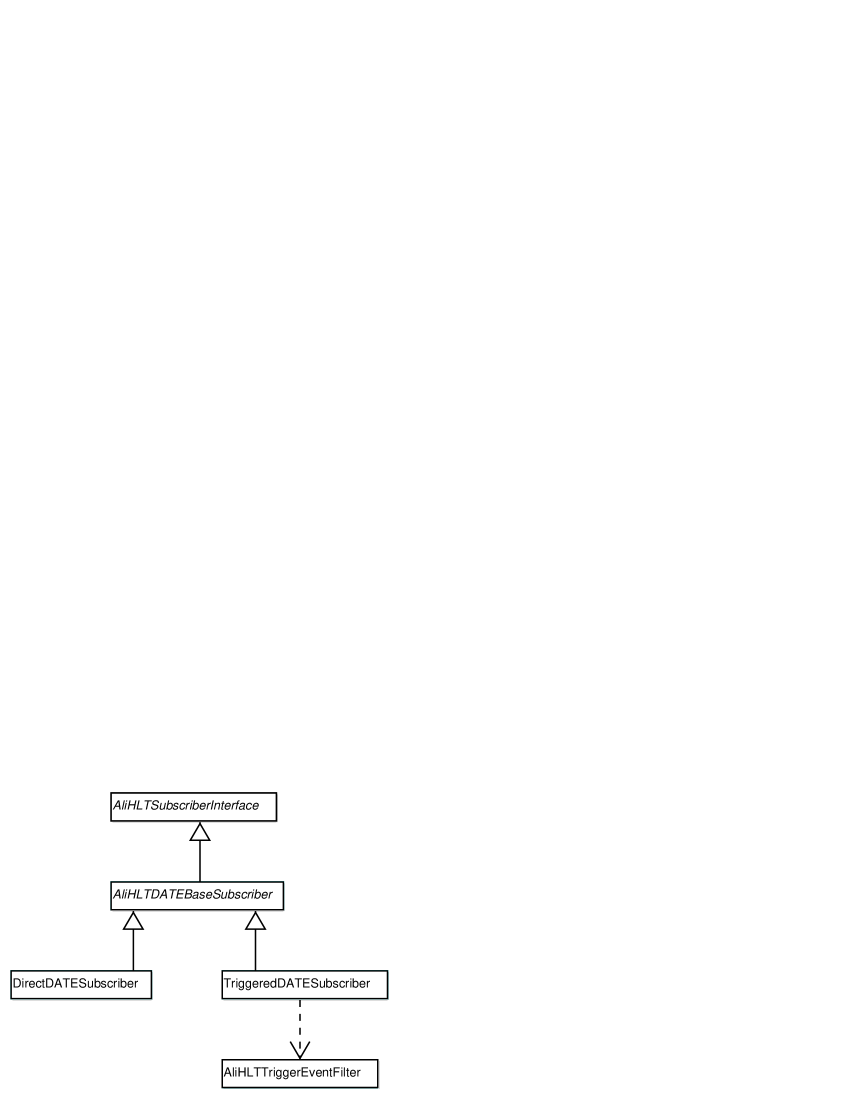
The first of the primary functions is Run, which has the purpose of initializing the library provided by DATE and starting the background thread that runs the DATEEventsDone function described later. It also interacts with the DATE run-control to inform it about the activation of a recording program. Run’s counterpart is the Stop method called at the end of a program. It terminates the started background thread, informs the run-control about the program’s end, and deinitializes the DATE library. To pass an event to the DATE system for recording the third function, SendEventToDATE, has to be called. Its main parameters are the ID of the event concerned, its corresponding sub-event descriptor, and a 32 bit unsigned integer containing additional event flags to pass to DATE.
In the current version this function imposes one restriction on the event data. The program is currently only able to create one type of DATE events, called streamlined events, in which the event data has to be prefixed directly by the DATE event header. As a consequence space has to be available in front of the data in shared memory for the appropriate amount of bytes so that an event header can be created there. In addition to the event ID the header contains the number of the GDC node where the event will be assembled as well as the additional flags that have been passed in the function’s parameter. The GDC ID is obtained by calling the class’s GetGDCID helper function. After calling the DATE function to record the event described by the constructed header, the function updates the run-control’s event and byte counters appropriately.
Running as a continuous loop in a background thread the DATEEventsDone function’s task is to query DATE via its library periodically for events that have already been recorded. For these finished events the publisher proxy’s EventDone function is called to allow the event’s original publisher to release it. This polling is done in configurable intervals, by default in half a seconds intervals. Next to the periodic check for recorded events the loop also queries run-control status flags to determine whether the program should continue running or whether it should terminate.
GetGDCID is a helper function to encapsulate the determining of the GDC ID to be used for an event. For tests the function currently implements a round-robin scheme based on an event’s ID and the number of active GDCs.
C.1.2 The Direct DATE Subscriber
In the DirectDATESubscriber component each event received by the components’s subscriber object is directly passed to DATE for recording. The NewEvent method implemented by the DirectDATESubscriber class directly calls the SendEventToDATE method provided by its AliHLTDATEBaseSubscriber parent class. Apart from setting up all necessary objects there is not much more functionality contained in this component.
C.1.3 The Triggered DATE Subscriber
Unlike the previous DirectDATESubscriber, the TriggeredDATESubscriber component does not forward each event to DATE immediately. Instead it uses an approach similar to the TriggeredFilter component from section 7.1.5. A new received event is entered into a list, and only upon receipt of event done data for it a decision is made which parts of the event are to be passed to DATE. It is possible that an event is not announced at all or only as an empty event with no data. Event done data for an event is received from another subscriber via the publisher component. The event trigger decision is made using an object of the AliHLTTriggerEventFilter class, also described in 7.1.5. In the EventDoneData function implemented by TriggeredDATESubscriber the filter object’s FilterEventDescriptor function is called to determine the data blocks to record. Similar to the trigger filter component the triggered DATE subscriber can also be configured to either forward untriggered events as empty events with no data blocks or to simply release them without invoking DATE.
Appendix D Glossar
- ACM
-
Association for Computing Machinery
- ADC
-
Analog to Digital Converter
- ALICE
-
A Large Ion Collider Experiment — Future heavy-ion experiment at CERN’s LHC Collider
- API
-
Application Programmer’s Interface
- ATLAS
-
A Toroidal LHC ApparatuS — Future general purpose experiment at CERN’s LHC Collider
- ATOLL
-
ATOmically Low Latencies — A SAN for the PCI bus being developed at the University of Mannheim
- BAR
-
Base Address Register
- BCL
-
Basic Communication Library — C++ communication class library covered in this thesis
- BLOB
-
Binary Large OBject
- BNL
-
Brookhaven National Laboratory
- C
-
Procedural programming language well suited to system programming
- C++
-
Programming language based on C with object-oriented extensions
- CAMAC
-
Computer Automated Measurement and Control — Industry standard instrumentation bus
- CBM
-
Compressed-Baryonic-Matter — Planned experiment at the future HESR accelerator at GSI
- CERN
-
European Organisation for Nuclear Research in Geneva, Switzerland
- CMS
-
Compact Muon Solenoid — Future general purpose experiment at CERN’s LHC Collider
- COTS
-
Commodity-Off-The-Shelf
- COW
-
Cluster Of Workstations
- CRC
-
Cyclic Redundancy Check
- CSMA/CD
-
Carrier Sense Multiple Access with Collision Detection — Ethernet technology for regulating access to physical transmission medium
- CSR
-
Configuration Space Register
- DAQ
-
Data AcQuisition
- DARPA
-
Defense Advanced Research Projects Agency
- DATE
-
ALICE Data Acquisition and Test Environment
- DCS
-
Detector Control System
- DDL
-
Detector Data Link
-
Specific energy loss of charged particles per distance travelled
- DMA
-
Direct Memory Access
-
Distribution of particles per unit of pseudo-rapidity
- EDM
-
Event Destination Manager
- EG
-
Event Gatherer
- EM
-
Event Merger
- ES
-
Event Scatterer
- FE
-
Fast Ethernet or Front End
- FEE
-
Front End Electronics
- FEP
-
Front End Processor
- FIFO
-
First-In-First-Out
- FMD
-
Forward Multiplicity Detector — One of ALICE’s detectors
- FPGA
-
Field Programmable Gate Array
- FSM
-
Finite State Machine
- FT
-
Fault Tolerance
- gcc
-
GNU C Compiler or GNU Compiler Collection
- GDC
-
Global Data Concentrator
- GNU
-
GNU’s Not Unix — Project to provide a freely available version of a Unix like operating system
- GSI
-
Gesellschaft für Schwerionenforschung in Darmstadt, Germany
- GbE
-
Gigabit Ethernet
- HADES
-
High Acceptance Di-Electron Spectrometer — Detector at GSI
- HESR
-
High Energy Storage Ring — Future Accelerator at GSI
- HI
-
Heavy-Ion
- HL
-
Hierarchy Level
- HLT
-
High Level Trigger
- HMPID
-
High Momentum Particle IDentification — One of ALICE’s detectors
- HPC
-
High Performance Computing
- I/O
-
Input & Output
- IEEE
-
Institute of Electrical and Electronics Engineers, Inc.
- IETF
-
Internet Engineering Task Force
- IIS-A
-
Fraunhofer-Institut für Integrierte Schaltungen
- IP
-
Internet Protocol
- ISA
-
Industry Standard Architecture — PC extension bus
- ITS
-
Inner Tracking System — One of ALICE’s detectors
- k
-
As a prefix usually , however in this thesis when used as prefix for bits or bytes or when used for counts of multiples of 2 (e.g. 32 or 128), means
- kB
-
Bytes
- L0
-
Level 0 Trigger
- L1
-
Level 1 Trigger
- L2
-
Level 2 Trigger
- L3
-
Level 3 Trigger
- LAM
-
Look At Me — An interrupt signal
- LAM/MPI
-
MPI implementation
- LDC
-
Local Data Concentrator
- LHC
-
Large Hadron Collider — Future accelerator at CERN
- LHCb
-
Large Hadron Collider beauty experiment — Future experiment dedicated to b-physics at CERN’s LHC Collider
- LSF
-
Load Sharing Facility
- M
-
As a prefix usually , however in this thesis when used as prefix for bits or bytes or when used for counts of multiples of 2 (e.g. 32 or 128), means
- MB
-
Bytes
- MCP
-
Micro Channel Plate — A technology for particle detectors
- MLUC
-
More or Less Useful Class Library — C++ utility class library covered in this thesis
- MP3
-
MPEG Audio Layer 3 — Compressed audio file format
- Molière radius
-
Material characteristic used to describe the transversal dimension of electromagnetic particle showers
- MPEG
-
Motion Picture Experts Group
- MPI
-
Message Passing Interface – Standard for parallel program communication
- MPICH
-
MPI implementation
- MTU
-
Maximum Transmission Unit
- Mutex
-
Mutual Exclusion Semaphore
- MWPC
-
Multi Wire Proportional Chamber — A technology for particle detectors
- NOW
-
Network Of Workstations
- Ogg Vorbis
-
Compressed audio file format
- OO
-
Object Oriented
- OOP
-
Object Oriented Programming
- PANDA
-
Proton-ANtiproton-at-DArmstadt — Planned experiment at the future HESR accelerator at GSI
- PBH
-
Publisher Bridge Head
- PC133
-
Specification for SDRAM modules with 133 MHz clock frequency
- PCI
-
Peripheral Component Interconnect — PC extension bus
- PCISIG
-
Peripheral Component Interconnect Special Interest Group — PCI standardization body
- PDS
-
Permanent Data Storage
- PHOS
-
PHOton Spectrometer — One of ALICE’s detectors
- PID
-
Particle IDentification
- PIO
-
Programmed I/O
- PM
-
Patch Merger
- PMD
-
Photon Multiplicity Detector — One of ALICE’s detectors
- PPC
-
Parallel Plate Counters — A technology for particle detectors
- Pseudo-rapidity
-
Variable for particles in a collision. Defined as , where is the angle between the particle and the direction of the undeflected beam. Approximates the relativistic rapidity of a particle.
- PSI
-
PCI and Shared memory Interface — Driver and library for PCI hardware and shared memory access covered in this thesis
-
Transversal Momentum
- PVM
-
Parallel Virtual Machine — Library for parallel program communication
- QGP
-
Quark-Gluon Plasma
- RFC
-
Request For Comment — Informal Internet standard
- RHIC
-
Relativistic Heavy Ion Collider — Accelerator at BNL
- RICH
-
Ring Image Čerenkov (or Cherenkov) Counter — A technology for particle detectors
- RORC
-
Read Out and Receiver Card
- RPC
-
Resistive Plate Chamber — A technology for particle detectors (In computing also Remote Procedure Call, but not used as such in this thesis)
- SAN
-
System Area Network
- SBH
-
Subscriber Bridge Head
- SCI
-
Scalable Coherent Interface — SAN technology
- SDD
-
Silicon Drift Detector — A technology for particle detectors
- SI95
-
SpecInt95 — Unit to measure computing speed
- SISCI
-
Software Infrastructure for SCI — SCI programming API
- SM
-
Slice Merger
- SMP
-
Symmetric Multi-Processor system - A system with multiple processors (CPUs) accessing the same memory
- SPD
-
Silicon Pixel Detector — A technology for particle detectors
- SPS
-
Super Proton Synchrotron — Accelerator at CERN
- SSD
-
Silicon Strip Detector — A technology for particle detectors
- SSI
-
Single System Image
- SSIC
-
Single System Image Cluster
- STAR
-
Solenoidal Tracker at RHIC — Detector at the RHIC accelerator at BNL
- STL
-
Standard Template Library
- ShM
-
Shared Memory
- Si
-
Silicon
- TCP
-
Transmission Control Protocol
- TDR
-
Technical Design Report
- TOF
-
Time Of Flight — One of ALICE’s detectors
- TPC
-
Time Projection Chamber — A technology for particle detectors as well as one of ALICE’s detectors
- TRD
-
Transition Radiation Detector — A technology for particle detectors as well as one of ALICE’s detectors
- UML
-
Unified Modelling Language
- VITA
-
VMEbus International Trade Association
- VMEbus
-
VERSAmodule Eurocard extension bus — Industry standard instrumentation bus
- WAN
-
Wide Area Network
- ZDC
-
Zero Degree Calorimeter — One of ALICE’s detectors
- ZN
-
Zero degree Neutron calorimeters
- ZP
-
Zero degree Proton calorimeters
References
- [1] T. E. Anderson, D. E. Culler, D. A. Patterson et al., A Case for Networks of Workstations: NOW, IEEE Micro, Feb, 1995
- [2] K. Castagnera, D. Cheng, R. Fatoohi, et al., Clustered Workstations and their Potential Role as High Speed Compute Processors, NAS Computational Services Technical Report RNS-94-003, NAS Systems Division, NASA Ames Research Center, April 1994.
- [3] T. Sterling, D. J. Becker, D. Savarese et al., Beowulf: A Parallel Workstation for Scientific Computation, Proceedings of the 24th International Conference on Parallel Processing, 1995
- [4] Linux Homepage: http://www.linux.org/ (June 2003)
- [5] http://www.kernel.org/ (November 2003)
- [6] kernel.org mirror sites: http://www.kernel.org/mirrors/ (November 2003)
-
[7]
R. M. Metcalfe and D. R. Boggs, Ethernet: Distributed Packet Switching for Local Computer Networks,
Communications of the ACM, Vol. 19, No. 5, July 1976 pages 395 - 404,
Available from http://www.acm.org/classics/apr96/ (June 2003) - [8] Multipoint data communications system with collision detection, US Patent number 4,063,220, December 1977
- [9] The Ethernet — A Local Area Network, Data Link Layer and Physical Layer Specifications, Version 1.0, September 1980, Digital Equipment Co., Intel Co., Xerox Co., “The Ethernet Blue Book”
- [10] Digital Equipment Corporation, Intel, Xerox, The Ethernet, Version 2.0, November 1982.
- [11] IEEE 802 Standard Family, Available from http://standards.ieee.org/getieee802/ (July 2003)
- [12] IEEE Standard 802.3: Carrier sense multiple access with collision detection (CSMA/CD) access method and physical layer specifications
-
[13]
IEEE Standard 1596-1992: IEEE Standard for Scalable Coherent Interface (SCI), 2000,
Available from http://shop.ieee.org/store/product.asp?prodno=SS94951 (June 2003) - [14] Myricom & Myrinet Homepage: http://www.myricom.com/ (June 2003)
- [15] ATOLL Homepage: http://www.atoll-net.de (June 2003)
- [16] U. Brüning and L. Schälicke, ATOLL: A high-performance communication device for parallel systems, Proceedings of the 1997 Conference on Advances in Parallel and Distributed Computing. March 1997, Shanghai, China, pages 228-234., IEEE Computer Society Press, 1997
- [17] L. Rzymianowicz, U. Brüning, J. Kluge et al., ATOLL: A Network on a Chip, Proceedings of the Cluster Computing Technical Session (CC-TEA) of the PDPTA’99 conference, June 28 - July 1 1999, in Las Vegas, NV.
- [18] G. E. Moore, Cramming more components onto integrated circuits, Electronics, Vol. 38, No. 8, April 1965, Available from http://www.intel.com/research/silicon/mooreslaw.htm (July 2003)
- [19] J. L. Hennessy and D. A. Patterson, Computer Architecture: A Quantitative Approach, Morgan Kaufman, CA, 1996, ISBN 1-55860-329-8, Chapter 5 “Memory-Hierarchy Design”
- [20] PCI Special Interest Group (PCISIG) Homepage: http://www.pcisig.com/ (June 2003)
-
[21]
PCI Local Bus Specification, Rev 2.3, The PCISIG,
Available from http://www.pcisig.com/specifications/order_form, Document NR16 (June 2003) -
[22]
Internet Engineering Task Force (IETF) Request For Comment (RFC) 793:
Transmission Control Protocol — DARPA Internet Program Protocol Specification, September 1981,
Available from http://rfc.net/rfc793.html (June 2003) - [23] FreeBSD Homepage: http://www.freebsd.org/ (June 2003)
- [24] OpenBSD Homepage: http://www.openbsd.org/ (June 2003)
- [25] Mosix Homepage: http://www.mosix.cs.huji.ac.il/ (June 2003)
- [26] A. Barak and O. La’adan, The MOSIX Multicomputer Operating System for High Performance Cluster Computing, Journal of Future Generation Computer Systems, Vol. 13, No. 4-5, pages 361-372, March 1998
- [27] A. Barak, O. La’adan and A. Shiloh, Scalable Cluster Computing with MOSIX for Linux, Proc. Linux Expo ’99, pages 95-100, Raleigh, N.C., May 1999
- [28] openMosix Homepage: http://openmosix.sourceforge.net/ (June 2003)
- [29] Compaq Homepage: http://www.compaq.com/ (Redirected to HP in June 2003)
- [30] Hewlett-Packard Homepage: http://www.hp.com/ (June 2003)
- [31] Single System Image Clusters (SSIC) Homepage: http://ssic-linux.sourceforge.net/ (June 2003)
-
[32]
Platform Computing Load Sharing Facility (LSF) Homepage:
http://www.platform.com/products/LSF/ (June 2003) - [33] Platform Computing Homepage: http://www.platform.com/ (June 2003)
- [34] Condor Homepage: http://www.cs.wisc.edu/condor/ (June 2003)
- [35] M. Litzkow, Remote Unix — Turning Idle Workstations into Cycle Servers, Proceedings of Usenix Summer Conference, pages 381-384, 1987
- [36] M. Litzkow, M. Livny, and M. Mutka, Condor — A Hunter of Idle Workstations, Proceedings of the 8th International Conference of Distributed Computing Systems, pages 104-111, June, 1988
- [37] The Message Passing Interface (MPI) Standard Homepage: http://www-unix.mcs.anl.gov/mpi/ (July 2003)
- [38] Message Passing Interface Forum Homepage: http://www.mpi-forum.org/ (July 2003)
- [39] Message Passing Interface Forum, MPI: A Message-Passing Interface Standard, Version 1.1, June 1995, Available from http://www.mpi-forum.org/docs/mpi-11-html/mpi-report.html (July 2003)
- [40] Message Passing Interface Forum, MPI-2: Extensions to the Message-Passing Interface, Available from http://www.mpi-forum.org/docs/mpi-20-html/mpi2-report.html (July 2003)
- [41] MPICH Homepage: http://www-unix.mcs.anl.gov/mpi/mpich/ (July 2003)
- [42] LAM/MPI Homepage: http://www.lam-mpi.org/ (July 2003)
- [43] PVM Homepage: http://www.epm.ornl.gov/pvm/pvm_home.html (July 2003)
-
[44]
IEEE Standard 1014-1987: IEEE Standard for A Versatile Backplane Bus: VMEbus, 1987,
Available from http://shop.ieee.org/store/product.asp?prodno=SS11544 (June 2003) - [45] VMEbus International Trade Association (VITA) Homepage: http://www.vita.com/ (June 2003)
-
[46]
An Introduction to VME,
Available from http://www.lecroy.com/lrs/appnotes/introvme/introvme.htm (June 2003) -
[47]
IEEE Standard 583-1982: IEEE Standard Modular Instrumentation and Digital Interface System
(CAMAC) (Computer Automated Measurement and Control), 1982,
Available from http://shop.ieee.org/store/product.asp?prodno=SS8524 (June 2003) -
[48]
An Introduction to CAMAC,
Available from http://www.lecroy.com/lrs/appnotes/introcam/introcam.htm (June 2003) - [49] VxWorks Homepage: http://www.windriver.com/products/vxworks5/index.html (June 2003)
- [50] LynxOS Homepage: http://www.lynuxworks.com/products/lynxos/lynxos.php3 (June 2003)
- [51] ALICE General Public Homepage: http://alice.web.cern.ch/ALICE/ (June 2003)
- [52] ALICE Homepage for Physicists: http://alice.web.cern.ch/ALICE/user.html (June 2003)
-
[53]
ALICE CERN Greybook Experiment Database entry:
http://graybook.cern.ch/programmes/experiments/ALICE.html (June 2003) - [54] The ALICE Collaboration, ALICE — Technical Proposal for A Large Ion Collider Experiment at the CERN LHC, CERN/LHCC/95-71 LHCC/P3, ISBN 92-9083-077-8, December 1995
-
[55]
CERN LHC Homepage:
http://lhc-new-homepage.web.cern.ch/lhc-new-homepage/ (June 2003) - [56] CERN Homepage: http://www.cern.ch/ (July 2003)
- [57] J. W. Harris and B. Müller, The Search for the Quark-Gluon Plasma, v2, arXiv number hep-ph/9602235, February. 1996, Available from http://www.arxiv.org/ (June 2003)
- [58] U. Heinze, Hunting Down the Quark-Gluon Plasma in Relativistic Heavy-Ion Collisions, v3, arXiv number hep-ph/9902424, March 1999, Available from http://www.arxiv.org/ (June 2003)
- [59] R. V. Gavai, Quark-Gluon-Plasma: Status of Heavy Ion Physics, v1, arXiv number hep-ph/0003147, March 2000, Available from http://www.arxiv.org/ (June 2003)
- [60] J.-P. Blaizot, Theory of the Quark-Gluon Plasma, v1, arXiv number hep-ph/0107131, July 2001, Available from http://www.arxiv.org/ (June 2003)
- [61] U. Heinze, From SPS to RHIC: Breaking the Barrier to the Quark-Gluon Plasma, v1, arXiv number hep-ph/0109006, September 2001, Available from http://www.arxiv.org/ (June 2003)
- [62] T. Matsui, Quest for the Quark-Gluon Plasma, v1, arXiv number nucl-th/0305096, May 2003, Available from http://www.arxiv.org/ (June 2003)
- [63] The ALICE Collaboration, ALICE — Technical Proposal for A Large Ion Collider Experiment at the CERN LHC, Chapter 2 “The Inner Tracking System”, CERN/LHCC/95-71 LHCC/P3, ISBN 92-9083-077-8, December 1995
- [64] The ALICE Collaboration, ALICE — Technical Proposal for A Large Ion Collider Experiment at the CERN LHC, Chapter 3 “The Time Projection Chamber”, CERN/LHCC/95-71 LHCC/P3, ISBN 92-9083-077-8, December 1995
- [65] The ALICE Collaboration, ALICE — Technical Design Report of the Time Projection Chamber, CERN/LHCC/2000-001, ALICE TDR 7, ISBN 92-9083-155-3, January 2000
- [66] Private Communication Anders Strand Vestbø
- [67] Private Communication Ulrich Frankenfeld
- [68] The ALICE Collaboration, A Transition Radiation Detector for Electron Identification within the ALICE Central Detector, Addendum to the ALICE Technical Proposal, CERN/LHCC 99-13 LHCC/P3-Addendum 2, May 1999
- [69] The ALICE Collaboration, ALICE Technical Design Report of the Transition Radiation Detector, CERN/LHCC/2001-021, ALICE TDR 9, ISBN 92-9083-184-7, October 2001
- [70] The ALICE Collaboration, ALICE — Technical Proposal for A Large Ion Collider Experiment at the CERN LHC, Chapter 4 “Particle Identification”, CERN/LHCC/95-71 LHCC/P3, ISBN 92-9083-077-8, December 1995
- [71] The ALICE Collaboration, ALICE — Technical Proposal for A Large Ion Collider Experiment at the CERN LHC, Chapter 5 “The Photon Spectrometer (PHOS)”, CERN/LHCC/95-71 LHCC/P3, ISBN 92-9083-077-8, December 1995
- [72] The ALICE Collaboration, ALICE — Technical Proposal for A Large Ion Collider Experiment at the CERN LHC, Chapter 6 “Muon Arm Integration”, CERN/LHCC/95-71 LHCC/P3, ISBN 92-9083-077-8, December 1995
- [73] The ALICE Collaboration, The forward muon spectrometer - Addendum to the ALICE Technical Proposal CERN/LHCC/96-32, LHCC/P3/Addendum 1, October 1996
- [74] The ALICE Collaboration, ALICE Technical Design Report of the Dimuon Forward Spectrometer, CERN/LHCC/99-22, ALICE TDR 5, ISBN 92-9083-148-0, August 1999
- [75] The ALICE Collaboration, Addendum to the ALICE Technical Design Report of the Dimuon Forward Spectrometer, CERN/LHCC/2000-046, Addendum 1 to ALICE TDR 5, ISBN 92-9083-173-1, December 2000
- [76] The ALICE Collaboration, ALICE — Technical Proposal for A Large Ion Collider Experiment at the CERN LHC, Chapter 7 “Other forward detectors”, CERN/LHCC/95-71 LHCC/P3, ISBN 92-9083-077-8, December 1995
- [77] The ALICE Collaboration, ALICE — Technical Proposal for A Large Ion Collider Experiment at the CERN LHC, Chapter 12 “Implementation”, Sections 12.3.1 - 12.3.4, CERN/LHCC/95-71 LHCC/P3, ISBN 92-9083-077-8, December 1995
- [78] L3 Experiment Homepage: http://l3.web.cern.ch/l3/ (June 2003)
-
[79]
L3 CERN Greybook Experiment Database entry:
http://graybook.cern.ch/programmes/experiments/L3.html (June 2003) - [80] The L3 Collaboration, The L3 Technical Proposal, CERN-LEPC-83-5 LEPC-P-4, May 1983, Available from http://weblib.cern.ch/format/showfull?uid=1932632&base=CERCER&sysnb=0218925& SESSIONID=58dce55cdadeb94dc387438dd8672d16 (June 2003)
- [81] The ALICE Collaboration, ALICE — Technical Proposal for A Large Ion Collider Experiment at the CERN LHC, Chapter 9 “The trigger”, CERN/LHCC/95-71 LHCC/P3, ISBN 92-9083-077-8, December 1995
- [82] The ALICE Collaboration, ALICE — Technical Proposal for A Large Ion Collider Experiment at the CERN LHC, Chapter 10 “Data Acquisition, Control, and Computing”, CERN/LHCC/95-71 LHCC/P3, ISBN 92-9083-077-8, December 1995
- [83] ALICE DAQ DATE Homepage: http://aldwww.cern.ch/ (June 2003)
- [84] J.Nelson, O.Villalobos Baillie, E.Denes, et al. (The ALICE Collaboration), The ALICE Data Acquisition System, Proceedings of the International Conference on Computing in High Energy Physics 1995 (CHEP ’95), Rio de Janeiro, Brazil, September 1995
- [85] The ALICE High Level Trigger Working Group, ALICE High-Level Trigger Conceptional Design, December 2002, Available from http://www.kip.uni-heidelberg.de/ti/HLT/concept.html (July 2003)
- [86] ALICE High Level Trigger Homepage: http://www.ti.uni-hd.de/HLT/ (July 2003)
-
[87]
Fraunhofer-Institut für Integrierte Schaltungen IIS-A — Arbeitsgruppe für Elektronische Medientechnologie,
Homepage: http://www.emt.iis.fhg.de/index-en.html (June 2003) -
[88]
Fraunhofer-Institut für Integrierte Schaltungen IIS-A — MPEG Audio Layer-3,
Homepage: http://www.iis.fraunhofer.de/amm/techinf/layer3/index.html (June 2003) - [89] Ogg Vorbis Homepage: http://www.vorbis.com/ (June 2003)
- [90] Dolphin Interconnect Homepage: http://www.dolphinics.com/
- [91] P. V. C. Hough, Method and means for recognizing complex patterns, US Patent 3 069 654, 1962
- [92] R. O. Duda, P. E. Hart, Use of the Hough Transformation to Detect Lines and Curves in Pictures, Communications of the ACM, Vol. 15, Issue 1, pages 11-15, 1972
- [93] Private Communication Markus W. Schulz
- [94] STAR Detector Homepage: http://www.bnl.gov/rhic/STAR.htm (June 2003)
- [95] RHIC Homepage: http://www.bnl.gov/RHIC/ (June 2003)
- [96] BNL Homepage: http://www.bnl.gov/ (June 2003)
- [97] The ALICE Collaboration, ALICE Technical Design Report of the Trigger, Data Acquisition, High-Level Trigger, and Control System CERN/LHCC 2003-062, ALICE TDR 10, ISBN 92-9083-217-7, To be published in January 2004
- [98] T. Smith, Managing Mature White Box Clusters at CERN, Proceedings of the Second Large Scale Cluster Computing Workshop, Fermilab National Accelerator Laboratory, October 2002, Available from http://conferences.fnal.gov/lccws/papers2/mon/LCW_White_Box.pdf (June 2003)
- [99] D. Long, A. Muir, and R. Golding, A longitudinal survey of Internet host reliability, Hewlett-Packard Laboratories — Concurrent Computing Department, HPL-CCD-95-4, February 1995
-
[100]
CBM Experiment Homepage:
http://www-new.gsi.de/zukunftsprojekt/experimente/CBM/index_e.html (June 2003) -
[101]
HESR Accelerator Homepage:
http://www-new.gsi.de/zukunftsprojekt/beschleunigeranlage_e.html (June 2003) - [102] GSI Homepage: http://www.gsi.de/ (October 2003)
-
[103]
PANDA Experiment Homepage:
http://www-new.gsi.de/zukunftsprojekt/experimente/hesr-panda/index_e.html (June 2003) - [104] ATLAS Experiment Homepage: http://atlas.web.cern.ch/Atlas/Welcome.html (July 2003)
-
[105]
ATLAS CERN Greybook Experiment Database entry:
http://greybook.cern.ch/programmes/experiments/ATLAS.html (July 2003) - [106] The ATLAS Collaboration, ATLAS — Technical Proposal for a General-Purpose pp Experiment at the Large Hadron Collider at CERN, CERN/LHCC/94-43 LHCC/P2, ISBN 92-9083-067-0, December 1994
- [107] CMS Experiment Homepage: http://cmsinfo.cern.ch/Welcome.html/ (July 2003)
-
[108]
CMS CERN Greybook Experiment Database entry:
http://greybook.cern.ch/programmes/experiments/CMS.html (July 2003) - [109] The CMS Collaboration, CMS — The Compact Muon Solenoid Technical Proposal, CERN/LHCC/94-38 LHCC/P1, ISBN 92-9083-068-9, December 1994
- [110] LHCb Experiment Homepage: http://lhcb.web.cern.ch/lhcb/ (July 2003)
-
[111]
LHCb CERN Greybook Experiment Database entry:
http://greybook.cern.ch/programmes/experiments/LHCB.html (July 2003) - [112] The LHCb Collaboration, LHCb Technical Proposal — A Large Hadron Collider Beauty Experiment for Precision Measurements of CP Violation and Rare Decays, CERN/LHCC/98-4 LHCC/P4, ISBN 92-9083-123-5, February 1998
- [113] C. Adler, J. Berger, M. Demello, et al., The proposed Level-3 Trigger System for STAR, IEEE Transactions on Nuclear Science, Vol. 47, No. 2, pages 358-361, April 2000
- [114] Private Communication Volker Lindenstruth
- [115] The ATLAS Collaboration, ATLAS High-Level Trigger, Data Acquisition and Controls Technical Design Report, July 2003, Available from http://atlas-proj-hltdaqdcs-tdr.web.cern.ch/ atlas-proj-hltdaqdcs-tdr/tdr-files.html (July 2003)
- [116] The CMS Collaboration, CMS TriDAS Project Technical Design Report, Volume 2: Data Acquisition and High-Level Trigger, CERN/LHCC/02-26, CMS TDR 6, December 2002
- [117] The LHCb Collaboration, LHCb Online System — Data Acquisition and Experiment Control Technical Design Report, CERN/LHCC/2001-40, LHCb TDR 7, December 2001
-
[118]
Big Physical Area Memory Patch:
http://www.polyware.nl/~middelink/En/hob-v4l.html#bigphysarea (June 2003) -
[119]
IEEE Standard 1003.1-2001 (Open Group Technical Standard, Issue 6):
Standard for Information Technology — Portable Operating System Interface (POSIX), 2001,
Available from http://shop.ieee.org/store/product.asp?prodno=SH94956 (June 2003) - [120] The Open Group Single Unix Specification Homepage: http://www.unix-systems.org/version3/ (June 2003)
-
[121]
The Open Group Single Unix Specification Online:
http://www.unix-systems.org/version3/online.html (June 2003) - [122] The Single UNIX Specification, Version 3 (8 Volumes on CD-ROM), The Open Group Publication T031, March 2003, Available at http://www.opengroup.org/products/publications/catalog/un.htm (June 2003)
- [123] E. Gamma, R. Helm, R. Johnson, J. Vlissides, Design patterns - elements of reusable object-oriented software, Addison-Wesley Professional, ISBN 02-0163-361-2, 1997
- [124] System V interprocess communication mechanisms manual page, ipc, section 5, Linux manual pages, November 1993
- [125] T. Shanley and D. Anderson, PCI System Architecture, Addison-Wesley Professional, ISBN 02-0130-974-2, August 1999
- [126] F. Giacomini, T. Amundsen, A. Bogaerts, et al., Low-level SCI software functional specification, Esprit Project 23174 — Software Infrastructure for SCI (SISCI), Version 2.1.1, March 1999
-
[127]
B. Hall, Beej’s Guide to Network Programming — Using Internet Sockets,
Available from http://www.ecst.csuchico.edu/~beej/guide/net/ (June 2003) - [128] T. Kientzle, Algorithm Alley — Cyclic Redundancy Check, Dr. Dobbs Journal, April 1997
- [129] U. Frankenfeld, D. Rohrich, B. Skaali, et al., High-level triggering in heavy ion experiments, IEEE Transaction on Nuclear Science, Proceedings of the IEEE Real-Time Conference 2001, Valencia, 2001
- [130] T. M. Steinbeck, V. Lindenstruth, D. Röhrich et. al., A Framework for Building Distributed Data Flow Chains in Clusters, Proceedings of the 6th International Conference on Applied Parallel Computing 2002 (PARA02), Espoo, Finland, 2002, Lecture Notes in Computer Science 2367, Springer Publishing, ISBN 3-540-43786-X, 2002
- [131] V. Lindenstruth, C. Loizides, D. Roehrich, et al., Online Pattern Recognition for the ALICE High Level Trigger, v1, Submitted to IEEE Transactions on Nuclear Science, Proceedings of IEEE Real-Time Conference 2003, Montréal, arXiv number physics/0307102, July 2003, Available from http://www.arxiv.org/ (July 2003)
-
[132]
EU DataGrid project work package 4 (Fabric Management),
Homepage: http://hep-proj-grid-fabric.web.cern.ch/hep-proj-grid-fabric/ (June 2003) - [133] German SuSE Homepage: http://www.suse.de/ (November 2003)
- [134] International SuSE Homepage: http://www.suse.com/ (November 2003)
-
[135]
Linux kernel version 2.4.18:
http://www.kernel.org/pub/linux/kernel/v2.4/linux-2.4.18.tar.bz2
(or use one of the mirrors sites from [6]) (November 2003) - [136] J. L. Hennessy and D. A. Patterson, Computer Architecture: A Quantitative Approach, Morgan Kaufman, CA, 1996, ISBN 1-55860-329-8, Excercises Chapter 5 “Memory-Hierarchy Design”
- [137] D. Bhandarkar and J. Ding, Performance Characterization of the PentiumPro Processor, Proceedings of the Third International Symposium on High Performance Computer Architecture, February 1997, San Antonio, Texas, USA, 1997, Available from http://www.computer.org/conferences/hpca97/77640288.pdf (October 2003)
-
[138]
J. Keshava and V. Pentkovski, Pentium III Processor Implementation Tradeoffs,
Intel Technology Journal, 2nd quarter 1999,
Available from http://www.intel.com/technology/itj/q21999/articles/art_2.htm
(October 2003) - [139] V. Lindenstruth, T. M. Steinbeck, and A. Wiebalck, Prozessor-Schwinger, Linux-Magazin 05/2003, Linux New Media AG, München, ISSN 1432-640-X, May 2003
- [140] V. Lindenstruth, T. M. Steinbeck, and A. Wiebalck, Fluctuating Processors, Linux-Magazine Issue 31, June 2003, Linux New Media AG, München, ISSN 1471-567-8, June 2003
-
[141]
Precise Accounting Kernel Patch:
http://www.ti.uni-hd.de/HLT/documentation/software-and-documentation.html
(October 2003) -
[142]
Broadcom drivers:
http://www.broadcom.com/drivers/downloaddrivers.php (November 2003) -
[143]
Broadcom 570x Linux driver:
http://www.broadcom.com/drivers/driver-sla.php?driver=570x-Linux (November 2003)