Efficient dot product over word-size finite fields

Abstract

We want to achieve efficiency for the exact computation of the dot product of two vectors over word size finite fields. We therefore compare the practical behaviors of a wide range of implementation techniques using different representations. The techniques used include floating point representations, discrete logarithms, tabulations, Montgomery reduction, delayed modulus.

1 Introduction

Dot product is the core of many linear algebra routines. Fast routines for matrix multiplication [4, §3.3.3], triangular system solving and matrix factorizations [5, §3.3] on the one hand, iterative methods on the other hand (see e.g. [13, 9, 6], etc.) make extensive usage of an efficient dot product over finite fields. In this paper, we compare the practical behavior of many implementations of this essential routine. Of course, this behavior is highly dependent on the machine arithmetic and on the finite field representations used. Section 2 therefore proposes several possible representations while section 3 presents some algorithms for the dot product itself. Experiments and choice of representation/algorithm are also presented in section 3.

2 Prime field representations

We present here various methods implementing seven of the basic arithmetic operations: the addition, the subtraction, the negation, the multiplication, the division, a multiplication followed by an addition ($r\leftarrow a*x+y$) or AXPY (also called “fused-mac” within hardware) and a multiplication followed by an in-place addition ($r\leftarrow a*x+r$) or AXPYIN. Within linear algebra in general (e.g. Gaussian elimination) and for dot product in particular, these last two operations are the most widely used. We now present different ways to implement these operations. The compiler used for the C/C++ programs was “gcc version 3.2.3 20030309 (Debian prerelease)”.

2.1 Classical representation with integer division

Zpz is the classical representation, with positive values between 0 and $p-1$, for $p$ the prime.

• Addition is a signed addition followed by a test. An additional subtraction of the modulus is made when necessary.

• Subtraction is similar.

• Multiplication is machine multiplication and machine remainder.

• Division is performed via the extended gcd algorithm.

• AXPY is a machine multiplication and a machine addition followed by only one machine remainder.

For the results to be correct, the intermediate AXPY value must not overflow. For a $m-$bit machine integer, the prime must therefore be below $2^{\frac{m-1}{2}}-1$ if signed values are used. For 32 and 64 bits this gives primes below $46337$ and below $3037000493$.

Note that with some care those operations can be extended to work with unsigned machine integers. The possible primes then being below $65521$ and $4294967291$.

2.2 Montgomery representation

To avoid the costly machine remainders, Montgomery designed another reduction [10]: when $gcd(p,B)=1$, $n_{im}\equiv-p^{-1}\mod B$ and $T$ is such that $0\leq T\leq pB$, if $U\equiv Tn_{im}\mod B$, then $(T+Up)/B$ is an integer and $(T+Up)/B\equiv TB^{-1}\mod p$. The idea of Montgomery is to set $B$ to half the word size so that multiplication and divisions by $B$ will just be shifts and remaindering by $B$ is just application of a bit-mask. Then, one can use the reduction to perform the remainderings by $p$. Indeed one shift, two bit-masks and two machine multiplications are very often much less expensive than a machine remaindering.

The idea is then to change the representation of the elements: every element $a$ is stored as $aB\mod p$. Then additions, subtractions are unchanged and the prime field multiplication is now a machine multiplication, followed by only one Montgomery reduction. Nevertheless, One has to be careful when implementing the AXPY operator since $axB^{2}$ cannot be added to $yB$ directly. Then the primes must verify $(p-1)^{2}+p*(B-1)<B^{2}$, which gives $p\leq 40499$ (resp. $p\leq 2654435761$) for $B=2^{16}$ (resp. $B=2^{32}$).

2.3 Floating point representation

Yet another way to perform the reduction is to use the floating point routines. According to [2, Table 3.1], for most of the architectures (alpha, amd, Pentium IV, Itanium, sun, etc.) those routines are faster than the integer ones (except for the Pentium III). The idea is then to compute $T\mod p$ by way of a precomputation of a high precision numerical inverse of $p$: $T\mod p=T-\lfloor T*\frac{1}{p}\rfloor*p$.

The idea here is that floating point division and truncation are quite fast when compared to machine remaindering. Now on floating point architectures the round-off can induce a $\pm 1$ error when the flooring is computed. This requires then an adjustment as implemented e.g. in Shoup’s NTL [11] :

  NTL’s floating point reduction  

  double P, invP, T;
  ...
  T  -= floor(T*invP)*P;
  if (T >= P)     T -= P;
  else if (T < 0) T += P;

 

2.4 Discrete logarithms

This representation is also known as Zech logarithms, see e.g. [3] and references therein. The idea is to use a generator of the multiplicative group, namely a primitive element. Then, every non zero element is a power of this primitive element and this exponent can be used as an internal representation:

$$\begin{cases}0&\text{if }x=0\\ q-1&\text{if }x=1\\ i&\text{if }x=g^{i}\text{and }1\leq i<q-1\end{cases}$$

Then many tricks can be used to perform the operations that require some extra tables see e.g. [7, 1]. This representation can be used for prime fields as well as for their extensions, we will therefore use the notation $\mathtt{GF}(q)$. The operations are then:

• Multiplication and division of invertible elements are just an index addition and subtraction modulo $\overline{q}=q-1$.

• Negation is identity in characteristic $2$ and addition of $i_{-1}=\frac{q-1}{2}$ modulo $\overline{q}=$ in odd characteristic.

• Addition is now quite complex. If $g^{i}$ and $g^{j}$ are invertibles to be added then their sum is $g^{i}+g^{j}=g^{i}(1+g^{j-i})$ which can be implemented using index addition and subtraction and access to a “plus one” table ($t\_plus1[]$) of size $q$ giving the exponent $h$ of any number of the form $1+g^{k}$, so that $g^{h}=1+g^{k}$.

Operation	Elements	Indices	Cost
			+/-	Tests	Accesses
Multiplication	$g^{i}*g^{j}$	$i+j\ (-\overline{q})$	1.5	1	0
Division	$g^{i}/g^{j}$	$i-j\ (+\overline{q})$	1.5	1	0
Negation	$-g^{i}$	$i-i_{-1}\ (+\overline{q})$	1.5	1	0
Addition	$g^{i}+g^{j}$	$k=j-i\ (+\overline{q})$
		$i+t\_plus1[k]\ (-\overline{q})$	3	2	1
Subtraction	$g^{i}-g^{j}$	$k=j-i+i_{-1}\ (\pm\overline{q})$
		$i+t\_plus1[k]\ (-\overline{q})$	3.75	2.875	1

Table 1: Number of elementary operations to implement Zech logarithms for an odd characteristic

Table 1 shows the number of elementary operations to implement Zech logarithms for an odd characteristic finite field. Only one table of size $q$ is considered. This number is divided into three types: mean number of exponent additions and subtractions (+/-), number of tests and number of table accesses.

We have counted $1.5$ index operations when a correction by $\overline{q}$ actually arises only for half the possible values. The fact that the mean number of index operations is 3.75 for the subtraction is easily proved in view of the possible values taken by $j-i+\frac{q-1}{2}$ for varying $i$ and $j$. In this case, $j-i+i_{-1}$ is between $-\frac{\overline{q}}{2}$ and $\frac{3\overline{q}}{2}$ and requires a correction by $\overline{q}$ only two eighth of the time as shown in figure 1 for $q=101$.

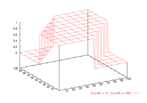
Figure 1: $j-i+\frac{q-1}{2}$ for $i$ and $j$ between $1$ and $q-1$, for $q=101$

The total number of additions or subtractions is then $2+0.25+1+0.5=3.75$ and the number of tests $1+0.875+1=2.875$ follows (one test towards zero, one only in case of a positive value i.e. seven eighth of the time, and a last one after the table lookup). It is possible to actually reduce the number of index exponents, (for instance replacing $i+x$ by $i+x-\frac{q-1}{2}$) but to the price of an extra test. In general, such a test ($a>q~{}?$) is as costly as the $a-q$ operation. We therefore propose an implementation minimizing the total cost with a single table.

These operations are valid as long as the index operations do not overflow, since those are just signed additions or subtractions. This gives maximal prime value of e.g. $1073741789$ for $32$ bits integer. However, the table size is now a limiting factor: indeed with a field of size $2^{26}$ the table is already $256$ Mb. Table reduction is then mandatory. We will not deal with such optimizations in this paper, see e.g. [8, 3] for more details.

2.4.1 Fully tabulated

A last possibility is to further tabulate the Zech logarithm representation. The idea is to code $0$ by $2\overline{q}$ instead of $0$. Then a table can be made for the multiplication:

• $t\_mul[k]=k$ for $0\leq k<\overline{q}$.

• $t\_mul[k]=k-\overline{q}$ for $q-1\leq k<2\overline{q}$.

• $t\_mul[k]=2\overline{q}$ for $2\overline{q}\leq k\leq 4\overline{q}$.

The same can be done for the division via a shift of the table and creation of the negative values, thus giving a table of size $5q$. For the addition, the $t\_plus1$ has also to be extended to other values, to a size of $4q$. For subtraction, an extra table of size $4q$ has also to be created. When adding the back and forth conversion tables, this gives a total of $15q$. This becomes quite huge and quite useless nowadays when memory accesses are a lot more expensive than arithmetic operations.

2.4.2 Field extensions

Another very interesting property is that whenever this implementation is not at all valid for non prime modulus, it remains identical for field extensions. In this case the classical representation would introduce polynomial arithmetic. This discrete logarithm representation, on the contrary, would remain atomic, thus inducing a speed-up factor of $O(d^{2})$, for $d$ the extension degree. See e.g. [4, §4] for more details.

2.5 Atomic comparisons

We first present a comparison between the preceding implementation possibilities. The idea is to compare just the atomic operations. “%” denotes an implementation using machine remaindering (machine division) for every operation. This is just to give a comparing scale. “NTL” denotes NTL’s floating point flooring for multiplication ; “Z/pZ” denotes our implementation of the classical representation when tests ensure that machine remaindering is used only when really needed. Last “GFq” denotes the discrete logarithm implementation of section 2.4. In order to be able to compare those single operations, the experiment is an application of the arithmetic operator on vectors of a given size (e.g. 256 for figures 2, 3 and 4).

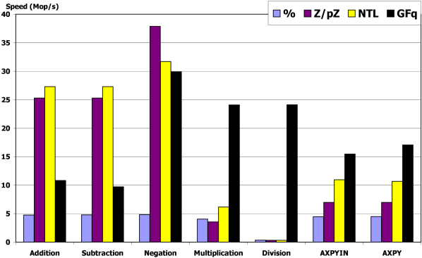
Figure 2: Single arithmetic operation modulo 32749 on a sparc ultra II, 250 MHz

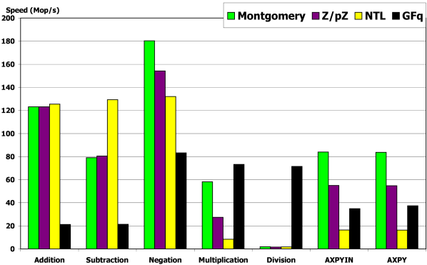
Figure 3: Single arithmetic operation modulo 32749 on a Pentium III, 1 GHz

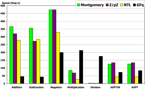
Figure 4: Single arithmetic operation modulo 32749 on a Pentium IV, 2.4 GHz

We compare the number of millions of field arithmetic operations per second, Mop/s.

Figure 2 shows the results on a UltraSparc II 250 Mhz. First one can see that the need of Euclid’s algorithm for the field division is a huge drawback of all the implementations save one. Indeed division over “GFq” are just an index subtraction. Next, we see that floating point operations are quite faster than integer operations: indeed, NTL’s multiplication is better than the integer one. Now, on this machine, memory accesses are not yet much slower than arithmetic operations. This is the reason why discrete logarithm addition is only 2 to 3 times slower than one arithmetic call. This, enables the “GFq” AXPY (base operation of most of the linear algebra operators) to be the fastest.

On newer PC, namely Intel Pentium III and IV of figures 3 and 4, one can see that now memory accesses have become much too slow. Then any tabulated implementation is penalized, except for extremely small modulus. NTL’s implementation is also penalized, both because of better integer operations and because of a pretty bad flooring (casting to integer) of the floating point representation. Now, for Montgomery reduction, this trick is very efficient for the multiplication. However; it seems that it becomes less useful as the machine division improves as shown by the AXPY results of figure 4. As shown section 2.2 the Montgomery AXPY is less impressive because one has to compute first the multiplication, one reduction and then only the addition and tests. This is due to our choice of representation $aB$. “Zpz”, not suffering from this distinction between multiplied and added values can perform the multiplication and addition before the reduction so that one test and sometimes a correction by $p$ are saved. Nevertheless, we will see in next section that our choice of representation is not anymore a disadvantage for the dot product.

3 Dot products

In this section, we extend the results of [4, §3.1]. To main techniques are used: regrouping operations before performing the remaindering, and performing this remaindering only on demand. Several new variants of the representations of section 2 are tested and compared. For “GFq” and “Montgomery” representations the dot products are of course performed with their representations. In particular the timings presented do not include conversions. The argument is that the dot product is computed to be used within another higher computation. Therefore the conversion will only be useful for reading the values in the beginning and for writing the result at the end of the whole program.

3.1 53 and 64 bits

The first idea is to use a representation where no overflow can occur during the course of the dot product so that the division is delayed to the end of the product: if the available mantissa is of $m$ bits and the modulo is $p$, the division happens at worst every $\lambda$ multiplications where $\lambda$ verifies the following condition:

$$\lambda(p-1)^{2}<2^{m}$$ (1)

For instance when using 64 bits integers with numbers modulo 40009, a dot product of vectors of size lower than $1.1510^{10}$ will never overflow. Therefore one has just to perform the AXPY without any division. A single machine remaindering is needed at the end for the whole computation. This produces very good speed ups for $53$ (double representation) and $64$ bits storage as shown in figure 5. There, the floating point representation performs the division “à la NTL” using a floating point precomputation of the inverse, so that it is slightly better than the $64-$bit integer representation. Note also the very good behavior of an implementation of P. Zimmermann [14] of Montgomery reduction over $32-$bit integers.

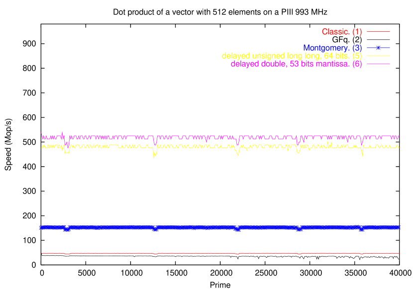
Figure 5: Dot product by delayed division, on a PIII

3.2 AXPY blocks

The extension of this idea is to specialize dot product in order to make several multiplications and additions before performing the division (which is then delayed), even with a small storage. Indeed, one needs to perform a division only when the intermediate result is able to overflow.

  Blocked dot product  

  res = 0;
  unsigned long i=0; if (K<DIM) while ( i < (DIM/K)*K ) {
      for(unsigned long j = 0; j < K; ++j, ++i) res += a[i]*b[i];
      res %= P;
  }
  for(; i< DIM; ++i) res += a[i]*b[i];
  res %= P;

 

This method will be referred as “block-XXX”. Figure 6 shows that this method is optimal for small primes since it performs nearly one arithmetic operation per processor cycle. Then, the step shape of the curve reflects the thresholds when an additional division is made.

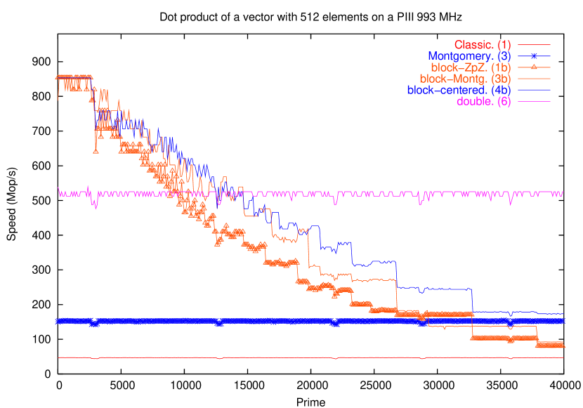
Figure 6: Dot product by blocked and delayed division, on a PIII

3.2.1 Choice of Montgomery representation

We see here, that our choice of representation ($aB$) for Montgomery is interesting. Indeed, the basic dot product operation is a cumulative AXPY. Now, each one of the added values is in fact the result of a multiplication. Therefore, the additions are between elements of the form $x_{i}B^{2}$, so that the reduction can indeed be delayed.

3.2.2 Centered representation

Another idea is to use a centered representation for “Z/pZ”: indeed if elements are stored between $-\frac{p-1}{2}$ and $\frac{p-1}{2}$, one can double the sizes of the blocks (equation 1 now becomes $\lambda_{centered}(\frac{p-1}{2})^{2}<2^{m-1}$).

3.3 Division on demand

The second idea is to let the overflow occur ! Then one should detect this overflow and correct the result if needed. Indeed, suppose that we have added a product $ab$ to the accumulated result $t$ and that an overflow has occurred. The variable $t$ now contains actually $t-2^{m}$. Well, the idea is just to precompute a correction $CORR=2^{m}\bmod p$ and add this correction whenever an overflow has occurred. Now for the overflow detection, we use the following trick: since $0<ab<2^{m}$, an overflow has occurred if and only if $t+ab<t$! The “Z/pZ” code now should look like the following:

  Overflow detection trick  

   sum = 0;
   for(unsigned long i = 0; i<DIM; ++i) {
         product = a[i]*b[i];
         sum += product;
         if (sum < product) sum += CORR;
   }

 

Of course one can also apply this trick to Montgomery reduction, but as shown in figure 6 the correction now implies two reductions at the end. Indeed the trick of using a representation storing $aB\mod p$ for any element $a$ enables to perform only one reduction at the end of each block. However at the end of the dot product, one reduction has to be performed to mod out the result, and an additional one to divide the element by $B$. Therefore, even though Montgomery reduction is slightly faster than machine remaindering, “overflow-Montgomery” performs $k+1$ reductions when “Z/pZ” performs only $k$ machine remaindering.

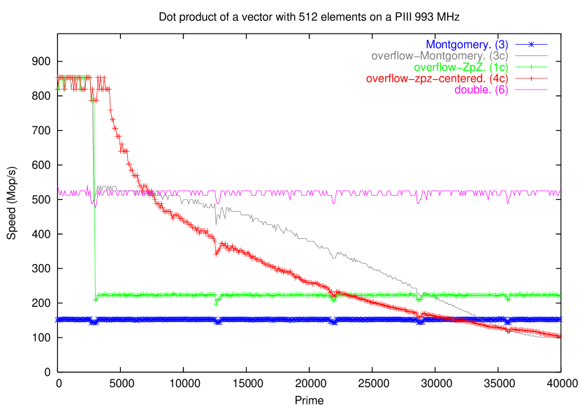
Figure 7: Overflow detection, on a PIII

The centered representation can be used also in this case. This gives the better performances for small primes. However, for this representation, the unsigned trick does not apply directly anymore. The overflow and underflow need to be detected each by two tests:

  Signed overflow detection trick  

         if      ((sum < product) && (product - sum < 0)) sum += CORR;
         else if ((product < sum) && (sum - product < 0)) sum -= CORR;
   }

 

Thus, the total of four tests is costlier and for bigger primes this overhead is too expensive.

3.4 Hybrid

Of course, one can mix both 3.2 and 3.3 approaches and delay even the overflow test when $p$ is small. One has just to slightly change the bound on $\lambda$ so that, when adding the correction, no new overflow occur:

$$\lambda(p-1)^{2}+(p-1)=\lambda p(p-1)<2^{m}.$$ (2)

This method will be referred as “block-overflow-XXX”.
We compared those ideas on a vector of size $512$ with $32$ bits (unsigned long on PIII). First, we see that as long as $512p(p-1)<2^{m}$, we obtain quasi optimal performances, since only one division is performed at the end. Then, when the prime exceeds the bound (i.e. for $p(p-1)>2^{32-9}$, which is $p>2897$) an extra division has to be made. On the one hand, this is dramatically shown by the drops of figure 7.

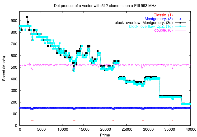
Figure 8: Block and overflow, on a PIII

On the other hand, however, those drops are levelled by our hybrid approach as shown in figure 8. There the step form of the curve shows that every time a supplementary division is added, performances drops accordingly. Now, as the prime size augments, the block management overhead becomes too important.

Unfortunately, an hybrid centered version is not useful. Even though the overflow-centered was the best of the overflow methods, a block version is of no use since the correction does not overflow towards zero. After the signed overflow trick (resp. underflow), the current sum is of value close to $-\frac{p-1}{2}$ or to $\frac{p-1}{2}$. Therefore no blocking can be made since a single new product in the bad direction would now induce an underflow (resp. overflow) !

Lastly, one can remark than no significant difference exist between the performances of “block-overflow-Zpz” and “block-overflow-Montgomery”. Indeed, the code is now exactly the same except for a single reduction for the whole dot product. This makes the Montgomery version better but only extremely slightly.

4 Conclusion

We have seen different ways to implement a dot product over word size finite fields. The conclusion is that most of the times, a floating point representation is the best implementation. This is even more the case for a Pentium IV 2.4 GHz, as shown figure 9.

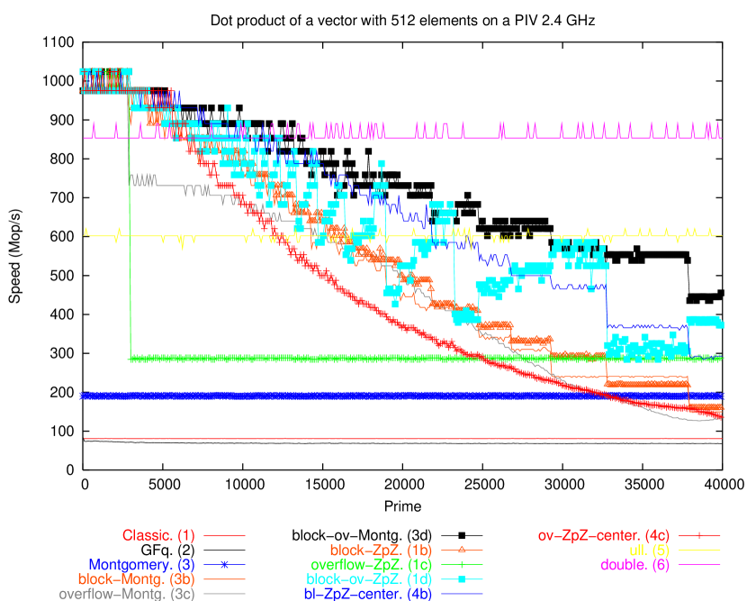
Figure 9: Hybrid, on a PIV 2.4 GHz

However, with some care, it is possible to improve this speed for small primes by a hybrid method using overflow detection and delayed division. Now, the floating point representation approximately doubles its performances on the PIV 2.4 GHz, when compared to the 1 GHz Pentium III. But surprisingly, the hybrid versions only slightly improve. Still and all, an optimal version should switch from block methods to a floating point representation according to the vector and prime size and to the architecture.

Nevertheless, bases for the construction of an optimal dot product over word size finite fields now exist: the idea is to use an Automated Empirical Optimization of Software [12] in order to produce a library which would determine and choose the best switching thresholds at install time.

References

- [1] Daniel V. Bailey and Christof Paar. Efficient arithmetic in finite field extensions with application in elliptic curve cryptography. Journal of Cryptology, 14(3):153–176, 2001.
- [2] David Defour. Fonctions l mentaires : algorithmes et impl mentations efficaces pour l’arrondi correct en double pr cision. PhD thesis, École Normale Supérieure de Lyon, September 2003.
- [3] Pierre Douillet. Zech logarithms and finite fields. Technical report, Faculté des Sciences, Paris, February 2001.
- [4] Jean-Guillaume Dumas, Thierry Gautier, and Clément Pernet. Finite field linear algebra subroutines. In Teo Mora, editor, Proceedings of the 2002 International Symposium on Symbolic and Algebraic Computation, Lille, France, pages 63–74. ACM Press, New York, July 2002.
- [5] Jean-Guillaume Dumas, Pascal Giorgi, and Clément Pernet. FFPACK: Finite field linear algebra package. In Jaime Gutierrez, editor, Proceedings of the 2004 International Symposium on Symbolic and Algebraic Computation, Santander, Spain. ACM Press, New York, July 2004.
- [6] Jean-Guillaume Dumas and Gilles Villard. Computing the rank of sparse matrices over finite fields. In Victor G. Ganzha, Ernst W. Mayr, and Evgenii V. Vorozhtsov, editors, Proceedings of the fifth International Workshop on Computer Algebra in Scientific Computing, Yalta, Ukraine, pages 47–62. Technische Universität München, Germany, September 2002.
- [7] Klaus Huber. Some comments on Zech’s logarithm. IEEE Transactions on Information Theory, IT–36:946–950, July 1990.
- [8] Klaus Huber. Solving equations in finite fields and some results concerning the structure of GF(). IEEE Transactions on Information Theory, IT–38:1154–1162, May 1992.
- [9] Brian A. LaMacchia and Andrew M. Odlyzko. Solving large sparse linear systems over finite fields. Lecture Notes in Computer Science, 537:109–133, 1991. http://www.research.att.com/∼amo/doc/arch/sparse.linear.eqs.ps.
- [10] Peter L. Montgomery. Modular multiplication without trial division. Mathematics of Computation, 44(170):519–521, April 1985.
- [11] Victor Shoup. NTL 5.3: A library for doing number theory, 2002. www.shoup.net/ntl.
- [12] R. Clint Whaley, Antoine Petitet, and Jack J. Dongarra. Automated empirical optimizations of software and the ATLAS project. Parallel Computing, 27(1–2):3–35, January 2001. www.elsevier.nl/gej-ng/10/35/21/47/25/23/article.pdf.
- [13] Douglas H. Wiedemann. Solving sparse linear equations over finite fields. IEEE Transactions on Information Theory, 32(1):54–62, January 1986.
- [14] Paul Zimmermann, 2002. Personal communication.