Search Efficiency in Indexing Structures for Similarity Searching

Abstract

Similarity searching finds application in a wide variety of domains including multilingual databases, computational biology, pattern recognition and text retrieval. Similarity is measured in terms of a distance function (edit distance) in general metric spaces, which is expensive to compute. Indexing techniques can be used reduce the number of distance computations. We present an analysis of various existing similarity indexing structures for the same. The performance obtained using the index structures studied was found to be unsatisfactory . We propose an indexing technique that combines the features of clustering with M tree(MTB) and the results indicate that this gives better performance.

1 Introduction

With the advent of new application domains such as multilingual databases, computational biology, text retrieval, pattern recognition and function approximation, there is a need for proximity searching, that is, searching for elements similar to a given query element. Similarity is modeled using a distance function; this distance function along with a set of objects defines a metric space. Computing distance function can be expensive, for example, one of the requirements in multilingual database systems is to find similar strings, where the distance(edit distance) between the strings is computed using an O(mn) algorithm where m, n are the length of the strings compared. This necessitates the use of an efficient indexing technique which would result in fewer distance computations at query time. Having an indexing structure serves the dual purpose of decreasing both CPU and I/O costs. Existing index structures such as B+ trees used in exact matching proves inadequate for the above requirements.

Various indexing structures have been proposed for similarity searching in metric spaces. We present the performance analysis of these structures in terms of the percentage of database scanned by varying edit distances from 10% to 100%.
After providing a preliminary background in Section 2, we move on to the description of the existing index structures in Section 3. Section 4 describes the experimental set up and the analysis is presented in Section 5. Section 6 concludes the paper.

2 Preliminaries

A metric space comprises of a collection of objects and an assosciated distance function satisfying the following properties.

• Symmetry
  $d(a,b)=d(b,a)$

• Non-negativity
  $d(a,b)>0$ if $(a\neq b)$ and $d(a,b)=0$ if $(a=b)$

• Triangle inequaltiy
  $d(a,b)\leq d(a,c)+d(c,b)$

a, b, c are objects of the metric space.

Edit distance(Levenshtein distance) satisfies the above mentioned properties. The edit distance between two strings is defined as the total number of simple edit operations such as additions, deletions and substitutions required to transform one string to another. For example, consider the strings paris and spire. The edit distance between these two strings is 4, as the transformation of paris to spire requires one addition, one deletion and two substitutions. Edit distance computation is expensive since the alogorithmic complexity is O(mn) where m, n are the length of the strings compared.

One of the common queries in applications requiring similarity search is to find all elements within a given edit distance to a given query string. Indexing structures for similarity search make use of the triangle inequality to prune the search space. Consider an element p with an assosciated subset of elements X such that
$\forall x\in X,d(p,x)<=k$

We want to find all strings within edit distance e from given query string q. That is reject all strings x such that

$$d(q,x)>e$$ (1)

From the triangle inequality, $d(q,p)\leq d(q,x)+d(x,p)$. Hence $d(q,x)\geq d(q,p)-d(x,p)$ which reduces to

$$d(q,x)\geq d(q,p)-k$$ (2)

From equations (1) and (2), the criterion reduces to

$$d(q,p)-k>e$$ (3)

If the inequality is satisfied, the entire subset X is eliminated from consideration.
However, we need to compute the O(mn) edit distance for all the elements in the subsets that do not satisfy the above criterion. [8] proposes bag distance which is given as

$$bag\_distance=max(|x-y|,|y-x|)$$ (4)

where $(x-y)$ is the set of the characters in x after dropping all common elements and $|x-y|$ gives the number of characters in (x-y). The algorithmic complexity for this computation is O(m+n) where $|x|$ = m, $|y|$ = n. Since $d_{bag}(x,y)\leq d_{edit}(x,y)$, bag distance can be used to filter out some of the candidate strings thereby reducing the search cost.

3 Index Structures

In this section, we provide a brief description of the data structures used for similarity indexing. Here,

• U is the set of all strings.

• n is the number of tuples in the dataset.

• B is the bucket size, i.e., the maximum number of tuples a leaf node can hold.

• d(a, b) is the edit distance between strings a and b.

• q is the query string.

• e is the search distance, i.e., all strings within an edit distance of e from q should be returned on a proximity search.

3.1 BK Tree

The Burkhard-Keller tree(BK tree) presented in [1] is probably the first general solution to search in metric spaces. A pivot element p is selected from the data set U and the dataset is partitioned into subsets $U_{i}$ such that ($\forall u\in U_{i},d(p,u)=i$). Each of the subsets is recursively partioned until there are no more than B elements in a subset.
For a given query and search distance, the search starts at the root(pivot element p) and traverses all subtrees at distance i such that

$$d(p,q)-e\leq i\leq d(p,q)+e$$ (5)

holds and proceed recursively till a leaf node is reached. In the leaf node, the query string is compared with all the elements.

3.2 FQ Tree

Fixed Queries trees [2] is a variation of BK trees. This tree is basically a BK tree where all the pivot elements at the same level are identical. The search algorithm is identical to that for BK trees. The benefit of FQ trees over BK trees is that some of the comparisons between the query string and the internal node pivots are saved along the backtracking that occurs in the tree.

3.3 FH Tree

In Fixed Height FQ trees [2], all leaves are at the same height. This makes some leaves deeper than necessary, but no additional costs are incurred as the comparison between the query and intermediate level pivot may already have been performed.

3.4 Bisector Tree

Bisector tree(BS tree) [9] is a binary tree built recursively as follows: Two routing objects $p_{1}$ and $p_{2}$ are chosen. While insertion, elements closer to $p_{1}$ are inserted in the left subtree and those closer to $p_{2}$ are inserted in the right subtree. For each routing object, the maximum covering radius($r_{i}$), i.e., the maximum distance of $p_{i}$ with any element in its subtree is stored. In our implementation, the distance of the element with its parent routing object is also stored. This helps in reducing some of the distance computations as shown in [4].
For a given query and edit distance, search starts at the root and recursively traverses the left subtree if

$$d(p_{1},q)-e\leq r_{1}$$ (6)

and the right subtree if a similar condition holds for $p_{2}$.

3.5 M Tree

The bisector tree can be extended to m-ary tree [4] by using m routing objects in the internal node instead of two. We select m routing objects for the first level. Together with each routing object is stored a covering radius that is the maximum distance of any object in the subtree associated with the routing object. A new element is compared against the m routing objects and inserted into the best subtree defined as that causing the subtree covering radius to expand less and in the case of ties selecting the closest representative. Thus it can be viewed that associated with each routing object $p_{i}$, is a region of the metric space Reg($p_{i})=(u\in U|d(p_{i},u)<r_{i}$) where $r_{i}$ is the covering radius. Further, each subtree is partitioned recursively.
In the internal node, $p_{i}$ and $r_{i}$ are stored together with a pointer to the associated subtree. Further to reduce distance computations M tree also stored precomputed distances between each routing object and its parent.
For a given query string and search distance, the search algorithm starts at the root node and recursively traverses all the paths for which the associated routing objects satisfy the following inequalities.

$$|d(p^{p}_{i},q)-d(p^{p}_{i},p_{i})|\leq r_{i}+e$$ (7)

and

$$d(p_{i},q)\leq r_{i}+e$$ (8)

In equation (7), we take advantage of the precomputed distance between the routing object and its parent.

3.6 VP Tree

Vantage Point tree(VP tree) [6] is basically a binary tree in which pivot elements called vantage points partition the data space into spherical cuts at each level to enable effective filtering in similarity search queries. It is built using a top down approach and proceeds as follows. A vantage point $S_{v}$ is chosen from the dataset and the distances between the vantage point and the elements in its subtree are computed. The elements are then grouped into the left and right subtrees based on the median of the distances, i.e., those elements whose distance from the vantage point is less than or equal to the median is inserted in the left subtree and others are inserted in the right subtree. This partitioning continues till the elements in the subtree fit in a leaf. The median value M is retained at each internal node to aid in the insertion and search process. In addition, each element in both the internal and leaf node holds the distance entries for every ancestor, which helps in cutting down the number of distance computations at query time. An optimized tree can be obtained by using heuristics to select better vantage points.
Search for a given query string starts at the root node. The distance between q and the vantage point at the node($S_{v}$) is computed and left subtree is recursively traversed if

$$d(q,S_{v})-e\leq M$$ (9)

Similarly, right subtree is traversed recursively if the following inequality holds.

$$d(q,S_{v})+e\geq M$$ (10)

Once a leaf node is reached, the query string need to be compared with all the elements in the leaf node, but some of the distance computations can be saved using the ancestral distance information.

3.7 MVP Tree

VP tree can be easily generalized to a multiway tree structure called Multiple Vantage Point tree [7]. A notable feature of MVP tree is that multiple vantage points can be chosen at each internal node and each of them can partition the data space into m groups. Hence it is required to store multiple cut off values instead of a single median value at each internal node. The various parameters that can be tuned to improve the efficiency of MVP tree are

• the number of vantage points at each internal node (v).

• the number of partitions created by each vantage point (m).

• the number of ancestral distances associated with each element in the leaf (p).

The insertion procedure starts by selecting a vantage point $S_{v1}$ from the dataset. The elements under the subtree of $S_{v1}$ are ordered with respect to their distances from $S_{v1}$ and partitioned into m groups. The m-1 cut off values are recorded at the internal node. The next vantage point $S_{v2}$ is a data point in the rightmost (m-1) partitions, which is farthest from $S_{v1}$ and it divides each of the m partitions into m subgroups. It can be observed that the nth vantage point is selected from the rightmost (m-n+1) partitions and the fan out at each internal node is $m^{v}$. This is continued until all elements in the subgroup fit in a leaf node. At the leaf, each element keeps information about its distance from its first p ancestors.

Given a query string q and an edit distance e, q is compared with the v vantage points at each internal node starting at the root. Let the distance between the vantage point $S_{vi}$ and q be d($S_{vi}$, q) and $M_{i}$ be the cut off value between subtrees $T_{i}$ and $T_{i+1}$. $T_{i}$ is recursively traversed if the both the inequalities

$$d(S_{vi},q)-e\leq M_{i}$$ (11)

and

$$d(S_{vi},q)+e\geq M_{i-1}$$ (12)

hold. For traversing the first subtree, only (11) need to be satisfied. Similarly, the inequality (12) is used to traverse the last subtree. A detailed description of the search procedure can be found in [7].

3.8 Clustering

Another technique used in similarity searching to reduce search cost is Clustering. Clustering partitions the collection of data elements into groups called clusters such that similar entities fall into the same group. Similarity is measured using the distance function, which satisfies the triangle inequality. A representative called clusteroid is chosen from each cluster. While searching, the query string is compared against the clusteroid and the associated cluster can be eliminated from consideration in case criterion (3) does not hold, which helps in reducing the search cost.
[3] proposes BUBBLE for clustering data sets in arbitrary metric spaces. The two distance measures used in the algorithm are given as

RowSum Let O = $O_{1},O_{2},...,O_{n}$ be a set of data elementsin metric space with distance function d. The rowsum of an object o $\in$ O is defined as RowSum(o) = $\Sigma_{j=1}^{n}d^{2}(O,O_{j})$. The clusteroid C is defined as the object C $\in$ O such that $\forall o\in O:RowSum(C)\leq RowSum(o)$.

Average Inter-Cluster Distance Let $O_{1}=\{O_{11},...,O_{1n_{1}}\}$ and $O_{2}=\{O_{21},...,O_{2n_{2}}\}$ be two clusters with number of elements n1 and n2 respectively. The average inter-cluster distance is defined as $D_{2}=\frac{\Sigma_{i=1}^{n_{1}}\Sigma_{j=1}^{n_{2}}d^{2}(O_{1i},O_{2j})}{n_{1}n_{2}}^{\frac{1}{2}}$.

Insertion in BUBBLE starts by creating a CF* tree, which is a height balanced tree. Each non-leaf node has entries of the form ($CF^{*}_{i}$, $child_{i}$) where $CF^{*}_{i}$ is the cluster feature, i.e., the summarized representation of the subtree pointed to by $child_{i}$. The leaf node entries are of the form ($CF^{*}_{i}$, $cluster_{i}$) where $CF^{*}_{i}$ is the clusteroid and $cluster_{i}$ points to the associated cluster. When an element x is to be inserted, it is compared against all the CF* entries in the internal node using the average inter-cluster distance $D_{2}$ and the child pointer associated with the closest CF* entry is followed. On reaching a leaf node, the cluster closest to x is the one having minimum RowSum value. If the distance between x and the closest clusteroid is less than a threshold value T, it is inserted in that cluster, a new clusteroid is selected and the CF* entries in the path from root to this leaf node are updated. In case the difference is greater than T, a new cluster is formed. In our implementation, each element entry in the cluster contains its distance with the clusteroid to reduce the number of distance computations.
For a given query string and search distance, the query is compared with all the clusteroids. If it does not satisfy the (3), the cluster elements need to be searched for similar strings. The precomputed distances can be used to eliminate some distance computations.

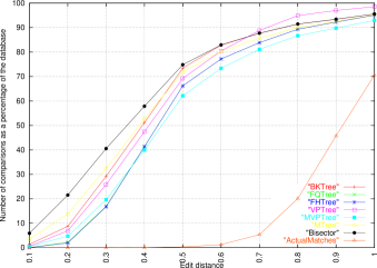
Figure 1: Performance Comparison of Similarity Indexing Structures

3.9 MTB

In case of M tree, a new element x is compared with the routing objects at the internal node and inserted into the best subtree. The best subtree is defined as the one for which the insertion of this element causes the least increase in the covering radius of the associated routing object. In the case of ties, the closest representative is selected. This continues until we reach a leaf node. This may cause physically close elements to fall into different subtrees. Along the path, the covering radii of the selected routing objects are updated if x is farther from p than any other element in its subtree. Thus there are no bounds on the covering radii associated with the routing objects. A possible optimzation is to bound the elements in the leaf nodes to be within a given THRESHOLD of the routing objects in its parent node. Also, the new element is inserted into the subtree associated with the closest routing object, there by keeping the physically close elements together. These two optimizations result in a new indexing structure, which we call M Tree with Bounds(MTB). Thus, in the case of MTB the insertion of an element that causes the covering radius of the routing object of the lowest level internal to exceed the THRESHOLD results in a partition of the leaf node entries such that the THRESHOLD requirements are maintained. Searching is similar to that of the basic tree implementation.

4 Experimental Setup

We have performed an analysis of the various similarity indexing structures described in the previous section. The metric used for comparing the performance is the percentage of the database scanned for a given query and search distance, which is a measure of the CPU cost incurred.
The experimental analysis were performed on a Pentium III(Coppermine) 768 MHz Celeron machine running Linux 2.4.18-14 with 512 MB RAM. All the indexing structures were implemented in C. The O(mn) dynamic programming algorithm to compute the edit distance between a pair of strings was used in the experiments. The dataset used for the analysis was an English dictionary dataset comprising of 100,000 words. The average word length of the dataset is around 9 characters. Six query sets each of 500 entries were chosen at random from the data set for the experiments. The results presented are obtained by averaging over the results for these query sets. The page size is assumed to be 4K bytes.

5 Analysis

In this section,we provide the analysis and the experimental results on the performance of the various similarity indexing structures. The implementation details of the various index structures are presented in the next subsection followed by the results.

5.1 Implementation Details

Assuming a page size of 4K bytes, the bucket size is taken to be 512 entries for BK tree, FQ tree and FH tree as each entry is 8 bytes. The routing data elements are chosen at random from the dataset.
The leaf node for VP tree as proposed in [6] has a single entry. The routing element is selected using the best spread heuristic [6]. For MVP trees, we ran the experiments for different values of parameters m, v and p and the values 2, 2 and 10 were shown to give better performance. For p = 10, the number of leaf node entries is found to be 110. The vantage point is selected at random for MVP tree.
In the case of bisector tree and M tree, the two farthest elements are chosen as pivot elements at the time of split of a FULL node. For M tree, we ran the experiment with the number of entries in the internal node m taking values 5 and 254.
In Clustering and Indexing with bounds, the THRESHOLD value used in our runs was chosen to be 5.

5.2 Experimental Results

5.2.1 Search complexity

In all the indexing structures, the criterion (3), which is obtained from the triangle inequality is used to prune the search space. As the search distance is increased, the number of pivots(or routing objects) that fail to satisfy the criterion (3) also increases resulting in an increase in the percentage of the database scanned.

Figure 1 shows the performance of the various similarity indexing structures with variation in the search distance. It can be seen that FQ tree and FH tree perform better than BK tree. This can be attributed to two reasons: The number of pivot element comparisons is less in case of FQ tree and FH tree as these trees have one fixed key per level. Whereas, in case of BK tree, there are as many distinct pivot elements per level as the number of nodes at that level. Further, FQ tree and FH tree use a better splitting technique resulting in more partitions as compared to BK tree. Hence, some of the partitions can be eliminated using (3).

Figure 2: Splitting characteristic of BKTree

Consider the case when a subset $C_{i}$ as shown in figure 2 is to be split in BK tree. Then the pivot element selected is some $c\in C_{i}$. Thus the maximum number of partitions that can result is 2i. However, in case of FQ tree, since a fixed pivot element is selected for each level, the chosen pivot is away from the subset, which may result in more partitions. It is shown in [6] that this results in better performance. In FH tree all the leaves are at the same level. Also, since we have already performed the comparison between the query and pivot of an intermediate level , we eliminate for free the need to consider a leaf. Hence FH tree performs slightly better than FQ tree.

Our implementation of VP tree uses the best spread heuristic [6] for selecting the vantage points. In addition, each internal node maintains the lower and upper bounds of the distance of elements in left and right subtrees. This can be used to cut down the distance computations using the triangle inequality. Because of these factors the performance is better as compared to BK tree. However, just like BK tree, as the vantage point is selected from the subset that is being partitioned and there are multiple distinct vantage points at any given level, FQ tree and FH tree show better performance.

As can be seen from the plots in Figure 1, MVP tree outperforms VP tree. Each leaf node entry in the MVP tree stores its distance to the first 10 ancestors. These precomputed distances help in reducing the search cost as compared to VP tree. In addition, MVP tree needs two vantage points to partition the data space into four regions whereas VP tree requires three vantage points for the same. This further reduces the number of distance computations at the internal nodes at search time. The left partition obtained using vantage point $S_{v1}$ is partitioned again using the farthest point $S_{v2}$ which is present in the right partition. Also, for smaller values of the edit distances($\leq 0.4$) the internal node comparisons dominate the results. In case of the MVP tree, since there are multiple keys at each internal node, it results in more distance computations as compared to the FH and FQ tree, which have one fixed key per level. This explains the crossover in the curves of the FQ tree, FH tree and MVP tree at search distance 0.4.

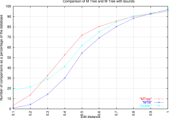
Figure 3: Performance Comparison of M Tree, Clustering and MTB

The clustering technique partitions the dataset into a fixed number of clusters $N_{c}$. This number varies inversely as the THRESHOLD i.e. the cluster radius. At search time, the query string is compared against each of the cluster representatives, the clusteroids. These comparisons are performed irrespective of the search distance. For a THRESHOLD of five, the clustering algorithm partitioned the dataset into 17,912 clusters. This explains the comparitively large number of searches for smaller values of search radii in figure 1. For clusteroids that do not satisfy the test in (3), the associated cluster elements are sequentially compared against the query string.

In the case of bisector tree, the insertion of a new data element may result in an increase in the covering radius of the routing object. The covering radii values depend upon the order in which the elements are inserted and may have large values.Due to this, at search time, a number of routing objects satisfy the test in equation (7). Thus, the Bisector Tree shows poor performance as compared to the other indexing structures. With M trees, even though the new element is inserted into a subtree such that the resulting increase in the covering radius is the least, there are no bounds on covering radius value. So the performance is identical to that of bisector tree. The poor performance can also be attributed to the presence of more number of routing objects to partition the data space.

It can be observed from the graph in Figure 3 that MTB that combines the features of M tree and clustering shows better performance. This can be attributed to the two optimzations used, which result in well formed clusters. For lower values of the search distance, the overhead of the comparisons with large number of routing objects at the internal nodes results in poor performance.

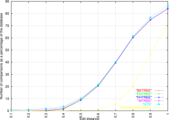
Figure 4: Performance Comparison of Indexing Structures using bag distance

The graph in Figure 4 shows comparison of the various indexing structures when bag distance computation is used to reduce some of the edit distance computations. The graph shows the edit distance computations needed with search distances varying from 10 to 100%.

Index Structure	Search Time (ms)
BK tree	0.5789
BK tree (with bag distance)	0.4164
FQ tree	0..5825
FQ tree (with bag distance)	0.4124
FH tree	0.5746
FH tree (with bag distance)	0.4090
VP tree	0.4951
M tree (with bag distance)	0.3041
Cluster	0.6531
MTB (with bag distance)	0.1465

Table 1: Time complexity

5.2.2 Search Time

Table 1 lists the average search time(ms) per query taken by various indexing structures. It can be observed that MTB tree takes comparatively lesser time. Bag distance computation helps in reducing the time complexity.

6 Conclusions and Future Work

We have presented a performance study of the search efficiency of similarity indexing structures. MTB, which combines the features of clustering and M tree is found to perform better than all the other indexing structures for most search distances. Bag distance computation, which is cheaper than edit distance computation, was used in the experiments. Its use resulted in reduced time complexity. Further, in applications where the required search distance is low and the string lengths are large, even better performance might result.

It can be observed that index structures like MVP tree, which make use of precomputed distances with ancestors to prune the search space perform better than others. In similarity searching, since multiple paths are traversed, keeping a fixed key per level as in FQ tree minimizes the search cost by reusing the precomputed distance at that level. Thus, reusing the pre computed distances results in better performance. Some indexed structures were shown to perform better with smaller values of edit distances($e\leq 0.3$) whereas some others perform better at higher values. It would be advantageous to maintain multiple index structures and depending upon the edit distance, select the appropriate one. Using cheaper distance computation algorithms can also significantly reduce the CPU cost. The quality of partioning is largely dependent on the heuristic used for selecting the pivots. As a future work, we propose to analyse the performance of various index structures with different heuristics.

7 Acknowledgement

We thank A Kumaran of Database Systems Lab, IISc for his advice during the work.

References

- [1] W. A. Burkhard, R. M. Keller, Some approaches to best-match file searching, Comm. of the ACM, 16(4):230–236, 1973.
- [2] R. Baeza-Yates, W. Cunto, U. Manber, S. Wu, Proximity matching using Fixed-queries trees, The 5th Combinatorial Pattern Matching, volume 807 of Lecture Notes in Computer Science, pages 198-212, 1994.
- [3] V. Ganti, R. Ramakrishnan, J. Gehrke, A. Powell, J. French, Clustering large datasets in arbitrary metric spaces, In the Proceedings of International Conference on Data Engineering, 1999.
- [4] P. Ciaccia, M. Patella, P. Zezula, M-tree: An efficient access method for similarity search in metric spaces, In Proceedings of the 23rd VLDB International Conference, Athens, Greece, September 1997.
- [5] Edgar Chavez, Gonzalo Navarro, Ricardo Baeza-Yates, Jose Luis Marroquin, Searching in Metric Spaces, ACM Computing Surveys, 1999.
- [6] Peter N. Yianilos, Data structures and algorithms for nearest neighbor search in general metric spaces, Proceedings of the fourth annual ACM-SIAM Symposium on Discrete algorithms, p.311-321, January 25-27, 1993.
- [7] Tolga Bozkaya, Meral Ozsoyoglu, Indexing Large Metric Spaces For Similarity Search Querie, ACM Transactions on Database Systems, Vol. 24, No. 3, Pages 361-404, September 1999.
- [8] Ilaria Bartolini, Paolo Ciaccia, Marco Patella, String Matching with Metric Trees Using an Approximate Distance, SPIRE 2002: 271-283.
- [9] I. Kalantari, G. McDonald, A data structure and an algorithm for the nearest point problem, IEEE Transactions on Software Engineering, 9(5), 1983.