Polymorphic Lemmas and Definitions in Prolog and Twelf
Abstract
Prolog is known to be well-suited for expressing and implementing logics and inference systems. We show that lemmas and definitions in such logics can be implemented with a great economy of expression. We encode a higher-order logic using an encoding that maps both terms and types of the object logic (higher-order logic) to terms of the metalanguage (Prolog). We discuss both the Terzo and Teyjus implementations of Prolog. We also encode the same logic in Twelf and compare the features of these two metalanguages for our purposes.
1 Introduction
It has long been the goal of mathematicians to minimize the set of assumptions and axioms in their systems. Implementers of theorem provers use this principle: they use a logic with as few inference rules as possible, and prove lemmas outside the core logic in preference to adding new inference rules. In applications of logic to computer security – such as proof-carrying code [Nec97] and distributed authentication frameworks [AF99a] – the implementation of the core logic is inside the trusted code base (TCB), while proofs need not be in the TCB because they can be checked.
Two aspects of the core logic are in the TCB: a set of logical connectives and inference rules, and a program in some underlying programming language that implements proof checking – that is, interpreting the inference rules and matching them against a theorem and its proof.
Definitions and lemmas are essential in constructing proofs of reasonable size and clarity. A proof system should have machinery for checking lemmas, and applying lemmas and definitions, in the checking of proofs. This machinery also is within the TCB; see Figure 1.
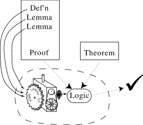
Trusted code base
Many theorem provers support definitions and lemmas and provide a variety of advanced features designed to help with tasks such as organizing definitions and lemmas into libraries, keeping track of dependencies, and providing modularization; in our work we are particularly concerned with separating that part of the machinery necessary for proof checking (i.e., in the TCB) from the programming-environment support that is used in proof development. This separation was particularly important for a proof-carrying code system we built initially in Prolog [AF00]. In this paper we will demonstrate a definition/lemma implementation that is about three dozen lines of code.
The Prolog language [NM88] has several features that allow concise and clean implementation of logics, proof checkers, and theorem provers [Fel93]. In a previous paper [AF99b], we presented a lemma and definition mechanism implemented in Prolog. In this paper, we extend that work and describe it more fully. We present the lemma mechanism and a generalization of our definition mechanism, again implemented in Prolog. Since we now have more experience using the Twelf system [Pfe91, PS99], we include a detailed comparison of the Twelf and Prolog versions of the encoding of our logic, lemmas, and definitions. An important purpose of this paper is to show which language features allow a small TCB and efficient representation of proofs. We also give a comparison of programming issues that are important to our proof-carrying code application.
Although the lemma and definition mechanism is general, we illustrate it using an implementation of higher-order logic. We call this logic the object logic to distinguish it from the metalogic implemented by Prolog or Twelf. Our object logic is not polymorphic, but our lemma and definition mechanisms are polymorphic in the sense that they can express properties that hold at any type of the object logic. The symmetry of equality, for example, is one such lemma we will encounter.
2 Encoding a higher-order logic
The Prolog version of the clauses we present use the syntax of the Terzo implementation [Wic99]. We also discuss the Teyjus implementation [NM99] and compare the two for our purposes. Terzo is interpreted and provides more flexibility, but Teyjus has a compiler in which our code runs much more efficiently.
Prolog is a higher-order logic programming language which extends Prolog in essentially two ways. First, it replaces first-order terms with the more expressive simply-typed -terms; Prolog implementations generally extend simple types to include ML-style prenex polymorphism [DM82, NP92]. Second, it permits implication and universal quantification (over objects of any type) in goal formulas.
We introduce types and constants using kind and type declarations, respectively. For example, a new primitive type and a new constant of type are declared as follows.
kind   t       type.
type   f       t -> t -> t.
Capital letters in type declarations denote type variables and are used in polymorphic types. In program goals and clauses, -abstraction is written using backslash \ as an infix operator. Capitalized tokens not bound by -abstraction denote free variables. All other unbound tokens denote constants. Universal quantification is written using the constant pi in conjunction with a -abstraction (e.g., pi X\ represents universal quantification over variable X). The symbols comma and => represent conjunction and implication. The symbol :- denotes the converse of => and is used to write the top-level implication in clauses. The type o is the type of clauses and goals of Prolog. We usually omit universal quantifiers at the top level in definite clauses, and assume implicit quantification over all free variables.
We will encode a natural deduction proof system for our higher-order object logic. (In our earlier work [AF99b], we implemented a sequent calculus version.) We implement a proof checker for this logic that is similar to the one described by Felty [Fel93]. Program 2 contains the type declarations used in our encoding.
kind  tp              type.
kind  tm              type.
kind  pf              type.

type  form            tp.
type  intty           tp.
type  arrow           tp -> tp -> tp.           infixr  arrow   8.
type  pair            tp -> tp -> tp.

type  eq              tp -> tm -> tm -> tm.
type  imp             tm -> tm -> tm.           infixr  imp     7.
type  forall          tp -> (tm -> tm) -> tm.
type  false           tm.

type  lam             (tm -> tm) -> tm.
type  app             tp -> tm -> tm -> tm.
type  mkpair          tm -> tm -> tm.
type  fst             tp -> tm -> tm.
type  snd             tp -> tm -> tm.

type  hastype         tm -> tp -> o.
type  proves          pf -> tm -> o.
type  assump          o -> o.

type  refl            pf.
type  beta            pf.
type  fstpair         pf.
type  sndpair         pf.
type  surjpair        pf.
type  congr           tp -> tm -> tm -> (tm -> tm) -> pf -> pf -> pf.
type  imp_i           (pf -> pf) -> pf.
type  imp_e           tm -> pf -> pf -> pf.
type  forall_i        (tm -> pf) -> pf.
type  forall_e        tp -> (tm -> tm) -> pf -> tm -> pf.
We introduce three primitive types: tp for object-level types, tm for object-level terms (including formulas) and pf for proofs in the object logic.
We introduce constants for the object-level type constructors. The main type constructor for our object language is the arrow constructor taking two types as arguments. We also include objects of type tp to represent base types, such as form and intty.
To represent formulas, we introduce constants such as imp to represent implication in the object logic, and eq which takes two terms and a type and is used to represent equality at any type. We use infix notation for the type arrow and binary logical connectives. The binding strength of each infix operator is declared using an infix declaration. The constant forall represents universal quantification. It takes a type representing the type of the bound variable and a functional argument, which allows object-level binding of variables by quantifiers to be defined in terms of meta-level -abstraction. An example of its use is the following formula, which expresses the commutativity of equality for integers:
forall intty (X\ forall intty (Y\ (eq intty X Y) imp (eq intty Y X))).
The parser uses the usual rule for the syntactic extent of a lambda, so this expression is equivalent to
forall intty X\ forall intty Y\ eq intty X Y imp eq intty Y X.
This use of higher-order data structures is called higher-order abstract syntax [PE88]; with it, we don’t need to describe the mechanics of substitution explicitly in the object logic [Fel93].
To represent terms, we introduce the app and lam constants for application and abstraction, as well as constants for pairing and projections. The app constructor takes three arguments. The second argument is a term of functional type and the third argument is the term it is applied to. The first argument is the type of the argument to the function. The lam constant has a type, which like forall, uses meta-level abstraction to represent object-level binding.
The constants at the end of Program 2 are used to build terms representing proofs. We call these constants as well as any other terms whose type ends in “-> pf” proof constructors.
hastype (eq T X Y) form :- hastype X T, hastype Y T.
hastype (A imp B) form :- hastype A form, hastype B form.
hastype (forall T A) form :- pi x\ (hastype x T => hastype (A x) form).
hastype false form.
hastype (lam F) (T1 arrow T2) :- pi x\ (hastype x T1 => hastype (F x) T2).
hastype (app T1 F X) T2 :- hastype F (T1 arrow T2), hastype X T1.
hastype (mkpair X Y) (pair T1 T2) :- hastype X T1, hastype Y T2.
hastype (fst T2 X) T1 :- hastype X (pair T1 T2).
hastype (snd T1 X) T2 :- hastype X (pair T1 T2).

proves Q A :- assump (proves Q A).
proves refl (eq T X X).
proves beta (eq T2 (app T1 (lam F) X) (F X)).
proves fstpair (eq T1 (fst T2 (mkpair X Y)) X).
proves sndpair (eq T2 (snd T1 (mkpair X Y)) Y).
proves surjpair (eq (pair T1 T2) (mkpair (fst T2 Z) (snd T1 Z)) Z).
proves (congr T X Z H P1 P2) (H X) :-
  hastype X T, hastype Z T,
  proves P1 (eq T X Z), proves P2 (H Z).
proves (imp_i Q) (A imp B) :-
  pi p\ (assump (proves p A) => proves (Q p) B).
proves (imp_e A Q1 Q2) B :-
  hastype A form, proves Q1 (A imp B), proves Q2 A.
proves (forall_i Q) (forall T A) :-
  pi y\ (hastype y T => proves (Q y) (A y)).
proves (forall_e T A Q X) (A X) :-
  pi x\ (hastype x T => hastype (A x) form),
  hastype X T,
  proves Q (forall T A).
Program 3 implements both typechecking and inference rules. The last four clauses of Program 3 implement the introduction and elimination rules for implication and universal quantification, which are given in Figure 4.
| # |
The -I rule has the proviso that the variable cannot appear free in , or in any assumption on which the deduction of depends.
We do not include inference rules for the other logical connectives. Instead, we define them in terms of existing connectives using our definition mechanism described later. The remaining clauses for the proves predicate implement inference rules for equality. Typechecking for terms is implemented by the hastype clauses. Proof checking is implemented by the proves clauses. A goal of the form (proves P A) should be run only after A is typechecked, i.e., a proper check has the form (hastype A form, proves P A).
To implement the discharge of assumptions in the implication introduction rule, we use implication and universal quantification in Prolog goals. The goal (D => G) adds clause D to the Prolog clause database, attempts to solve G, and then (upon either the success or failure of G) removes D from the clause database. The goal (pi y\(G y)) introduces a new constant c with the same type as y, replaces y with c, and attempts to solve the goal (G c). For example, consider the goal
proves (imp_i q\q) (a imp a)
where a is a propositional constant (a constant of type form); then Prolog will execute the (instantiated) body of the imp_i clause
pi p\ (assump (proves p a) => proves ((q\q) p) a)
This generates a new constant c, and adds (assump (proves c a) to the database; then the subgoal (proves ((q\q) c) a), which is -equivalent to (proves c a), matches the first clause for the proves predicate. The subgoal (assump (proves c a)) is generated and this goal matches our dynamically added clause. We have chosen to use the assump predicate for adding atomic clauses to the program. This is not necessary, but we find it useful to distinguish between adding atomic clauses and adding non-atomic clauses, which we will see later. Note that the typechecking clauses for forall and lam use meta-level implication and universal quantification in a manner similar to the proves clause for the -I rule.
It is important to show that our encoding of higher-order logic in Prolog is adequate. To do so, we must show that a formula has a natural deduction proof if and only if its representation as a term has an associated proof term that can be checked using the inference rules of Program 3. The encoding we use is similar to the encoding of higher-order logic in the Logical Framework [HHP93] and the proof of adequacy of our encoding is similar to the one discussed there. The main difference between the two encodings is the types of the logical connectives. For example, in their encoding, imp is given type tm and the fact that it is a connective which takes two formulas as arguments is expressed using object level types; the hastype clause is
hastype imp (form arrow form arrow form).
An implication must then be expressed using the app constructor, e.g., (app (app imp A) B). We found that this encoding of the connectives quickly became cumbersome and our encoding was more readable. On the other hand, our encoding is not as economical as the one we used previously [AF99b]. There we represented object-level types as meta-level types, which allowed us to eliminate all the hastype clauses and subgoals. The types of our object logic, however, did not match up well with the types of Prolog, which forced certain limitations in the implementation of our proof-carrying code system. (See Appel and Felty [AF99b] for further analysis.) The encoding in the current paper seems to be the best compromise.
3 Lemmas
In mathematics the use of lemmas can make a proof more readable by structuring the proof, especially when the lemma corresponds to some intuitive property. For automated proof checking (in contrast to automated or traditional theorem proving) this use of lemmas is not essential, because the computer doesn’t need to understand the proof in order to check it. But lemmas can also reduce the size of a proof (and therefore the time required for proof checking): when a lemma is used multiple times it acts as a kind of “subroutine.” This is particularly important in applications like proof-carrying code where proofs are transmitted over networks to clients who check them. We first present an example which we use to illustrate our lemma mechanism in Prolog (Section 3.1), and then present this mechanism as we’d implement it in Terzo (Section 3.2). We then explain the modifications required to meet the extra restrictions imposed by Teyjus (Section 3.3). We end this section with some optimizations that are important for keeping proofs that use lemmas as small as possible (Section 3.4) and then with some more examples (Section 3.5).
3.1 An example
Theorem 5 shows the use of our core logic to express a simple proof checking goal.
proves
  (forall_i I\ (forall_i J\ (imp_i Q\
    (congr intty I J (eq intty J) Q refl))))
  (forall intty I\ forall intty J\ (eq intty I J imp eq intty J I)).
The proof of this lemma uses the -I rule as well as congruence and reflexivity of equality. Its proof can be checked as a successful Prolog query to our core logic in Programs 2 and 3. Alternatively, we may want to prove it using the following general lemma about symmetry of equality at any type.
The proof of this lemma can be checked as the following Prolog query.
pi T\ pi A\ pi B\ pi P\
  (hastype A T, hastype B T, proves P (eq T B A)) =>
    proves (congr T B A (eq T A) P refl) (eq T A B).
This query introduces an arbitrary P, adds the typing clauses (hastype A T) and (hastype B T), and the assumption (proves P (eq T B A)) to the set of clauses, then checks the proof of congruence using these facts. The syntax => means exactly the same as :- , so we could just as well write this query as
pi T\ pi A\ pi B\ pi P\
  (proves (congr T B A (eq T A) P refl) (eq T A B) :-
     hastype A T, hastype B T, proves P (eq T B A)).
Now, suppose we abstract the proof (roughly, congr T B A (eq T A) P refl) from this query.
(Inference = (PCon\ pi T\ pi A\ pi B\ pi P\
               proves (PCon T A B P) (eq T A B) :-
                 hastype A T, hastype B T, proves P (eq T B A)),
 Proof = (T\A\B\P\ congr T B A (eq T A) P refl),
 Query = (Inference Proof),
 Query).
The solution of this query proceeds in four steps: the variable Inference is unified with a -term; Proof is unified with a -term; Query is unified with the application of Inference to Proof (which is a term -equivalent to the query of the previous paragraph), and finally Query is solved as a goal (checking the proof of the lemma).
Once we know that the lemma is valid, we can make a new Prolog atom symm to stand for its proof, and we can prove some other theorem in a context where the clause (Inference symm) is in the clause database; remember that (Inference symm) is -equivalent to
pi T\ pi A\ pi B\ pi P\
 (proves (symm T A B P) (eq T A B) :-
   hastype A T, hastype B T, proves P (eq T B A)).
This series of transformations starting with a proof checking subgoal has led us to a clause that looks remarkably like an inference rule. With this clause in the database, we can use the new proof constructor symm just as if it were primitive. Instead of adding new clauses like this to our proof checker, which would increase the size of our TCB, we show how to put such lemmas inside proofs.
3.2 Lemmas in proofs
In the example in the previous section, symm is a new constant, but when lemmas are proved and put inside proofs dynamically, we can instead “make a new atom” by simply pi-binding it. This leads to the recipe for lemmas shown in Program 6, which is the heart of our lemma mechanism.
type  lemma_pf  (A -> o) -> A -> (A -> pf) -> pf.

proves (lemma_pf Inference LemmaProof RestProof) C :-
 Inference LemmaProof,
 pi Name\ ((Inference Name) => (proves (RestProof Name) C)).
(We will improve it slightly in the next section.) This program introduces a constructor lemma_pf for storing lemmas in proofs. This constructor takes three arguments: (1) a derived inference rule Inference (of type A -> o) parameterized by a proof constructor (of type A), (2) a term LemmaProof of type A representing a proof of the lemma built from core-logic proof constructors (or using other lemmas), and (3) a proof of the main theorem RestProof that is parameterized by a proof constructor (of type A). Operationally, this clause first executes (Inference LemmaProof) as a query, to check the proof of the lemma itself; then it pi-binds Name in the lemma, adds it as a new clause, and runs RestProof (which is parameterized on the lemma proof constructor) applied to Name.
The terms Inference and Proof from the example in Section 3.1 illustrate the form of the terms which will appear as the first two arguments to lemma_pf. Theorem 7 illustrates the use of lemma_pf in an example; this theorem is a modification of Theorem 5 that uses the symm lemma.
proves
(lemma_pf
  (Symm\ pi T\ pi A\ pi B\ pi P\
    proves (Symm T A B P) (eq T A B) :-
        hastype A T, hastype B T, proves P (eq T B A))
  (T\A\B\P\ (congr T B A (eq T A) P refl))
  (symm\ (forall_i I\ (forall_i J\ (imp_i Q\ (symm intty J I Q))))))
(forall intty I\ forall intty J\ (eq intty I J imp eq intty J I)).
3.3 Lemmas in Teyjus
If we restrict ourselves to the Terzo implementation of Prolog, then meta-level formulas can occur inside proofs using any of the Prolog connectives. But if we want to be able to use Teyjus as well, we must make one more change. The Teyjus system does not allow => or :- to appear in arguments of predicates. Thus the term
  (Symm\ pi T\ pi A\ pi B\ pi P\
    proves (Symm T A B P) (eq T A B) :-
        hastype A T, hastype B T, proves P (eq T B A))
occurring in the symm lemma in Theorem 7 cannot appear directly as the first argument to lemma_pf. Teyjus also does not allow variables to appear at the head of the left of an implication. These restrictions come from the theory underlying Prolog [MNPS91]; without the latter one, a runtime check is needed to insure that every dynamically created goal is an acceptable one.
We can avoid putting :- inside arguments of predicates by writing the above term as
  (Symm\ pi T\ pi A\ pi B\ pi P\
    proves (Symm T A B P) (eq T A B) <<==
        hastype A T, hastype B T, proves P (eq T B A))
where <<== is a new infix operator of type o -> o. But this, in turn, means that the subgoal (Inference LemmaProof) of the lemma_pf clause in Program 6 will no longer check the lemma, since <<== has no operational meaning. To handle such goals, we add the three constants declared at the beginning of Program 8, which introduce both forward and backward implication arrows, and a new atomic predicate cl of type o -> o, and we introduce the two clauses that follow these declarations to interpret our new arrows as Prolog implication.
type  ==>>            o -> o -> o.              infixr  ==>>    4.
type  <<==            o -> o -> o.              infixl  <<==    0.
type  cl              o -> o.

(D ==>> G) :- (cl D) => G.
(G <<== D) :- (cl D) => G.

type  backchain    o -> o -> o.

proves P A :- cl Cl, backchain (proves P A) Cl.
hastype X T :- cl Cl, backchain (hastype X T) Cl.
assump G :- cl Cl, backchain (assump G) Cl.

backchain G G.
backchain G (pi D) :- backchain G (D X).
backchain G (A,B) :-  backchain G A; backchain G B.
backchain G (H <<== G1) :-  backchain G H, G1.
backchain G (G1 ==>> H) :-  backchain G H, G1.
Note that although it would have been more direct, we did not add:
(D ==>> G) :- D => G.
because of the Teyjus restriction mentioned above that variables cannot appear at the head of the left of an implication. The use of the cl “wrapper” solves the problem created by this restriction, but requires us to implement an interpreter to handle clauses of the form (cl A). The remaining clauses in Program 8 implement this interpreter.
Since the type of (Inference Proof) is o, the term Inference might conceivably contain subterms which are Prolog clauses. Of course, in Teyjus these clauses will not contain :- or =>, but they may contain <<== and ==>>, which get interpreted via the clauses of Program 8. They could also, for example, contain any other Prolog code including input/output operations. Executing (Inference Proof) cannot lead to unsoundness – if the resulting proof checks, it is still valid. But there are some contexts where we wish to restrict the kind of program that can occur inside a proof and be run when the proof is checked. For example, in a proof-carrying-code system, the code consumer might not want proof checking to cause Prolog to execute code that accesses private local resources.
To limit the kind and amount of execution possible in the executable part of a lemma, we introduce the valid_clause predicate of type o -> o (Program 9).
valid_clause (pi C) :-     pi X\ valid_clause (C X).
valid_clause (A,B) :-      valid_clause A, valid_clause B.
valid_clause (A <<== B) :- valid_clause A, valid_clause B.
valid_clause (A ==>> B) :- valid_clause A, valid_clause B.
valid_clause (proves Q A).
valid_clause (hastype X T).
valid_clause (assump (proves Q A)).
A clause is valid if it contains pi, comma, <<==, ==>>, proves, hastype, assump, and nothing else. Of course, a proves or assump clause contains subexpressions of type pf and tm, and a hastype clause has subexpressions of type tm and tp, so all the constants in proofs, terms, and types of our object logic are also permitted. Absent from this list are Prolog input/output (such as print) and the semicolon (backtracking search).
The valid_clause restriction is the reason that we only need new clauses for the proves, hastype, and assump predicates in Program 8. We must add at least these three because they are used for checking nodes in a proof that require using the clauses added dynamically via the cl predicate. Including no other predicates in the valid_clause definition guarantees that we need no other new clauses with cl subgoals.
Because of the introduction of <<==, ==>>, and valid_clause, we modify the clause in Program 6 for checking lemmas. The new clause is shown in Program 10.
proves (lemma_pf Inference LemmaProof RestProof) C :-
 pi Name\ (valid_clause (Inference Name)),
 Inference LemmaProof,
 pi Name\ (cl (Inference Name) => (proves (RestProof Name) C)).
The first subgoal is new; it pi-binds Name and checks to see if the new lemma applied to Name is valid. The only other modification is in the last subgoal, which adds the lemma as a new clause via the cl predicate. Since all lemmas will be added via cl, the only way to use them is via the proves clause in Program 8. Using that clause, the (cl Cl) subgoal looks up the lemmas that have been added, one at a time, and tries them out via the backchain predicate. This predicate processes the clauses in a manner similar to the Prolog language itself. In Terzo, using this interpreter is less efficient than the direct implementation in Program 6. In Teyjus, the interpreter is required, but when compiled, the code runs faster than either Terzo version.
In summary, our technique allows lemmas to be contained within the proof. We do not need to install new “global” lemmas into the proof checker. The dynamic scoping also means that the lemmas of one proof cannot interfere with the lemmas of another, even if they have the same names. This machinery uses several interesting features of Prolog:
Polymorphism.
The type of the lemma_pf constructor uses polymorphism to indicate that proof constructors introduced for lemmas can have different types.
Meta-level formulas as terms.
Lemmas such as symmetry of equality occur inside proofs as an argument to the lemma_pf constructor in the following form.
  (Symm\ pi T\ pi A\ pi B\ pi P\
    proves (Symm T A B P) (eq T A B) <<==
        hastype A T, hastype B T, proves P (eq T B A))
It is just a data structure (parameterized by Symm); it does not “execute” anything, in spite of the fact that it contains the Prolog quantifier pi and our new connective <<==. This gives us the freedom to write lemmas using syntax very similar to that used for writing primitive inference rules. Handling the new constants for <<== and ==>> is easy enough operationally. However, it is an inconvenience for the user, who must use different syntax in lemmas than in inference rules. This inconvenience is avoided in Terzo.
Dynamically constructed goals.
When the clause from Program 10 for the lemma_pf proof constructor checks the proof of a lemma by executing the goal (Inference LemmaProof), we are executing a goal that is built from a run-time-constructed data structure. Inference will be instantiated with terms such as the one above representing the symmetry lemma. It is only when such a term is applied to its proof and thus appears in “goal position” that it becomes the current subgoal on the execution stack.
Dynamically constructed clauses.
When, having successfully checked the proof of a lemma, the lemma_pf clause executes
cl (Inference Name) => (proves (RestProof Name) C)
it is adding a dynamically constructed clause to the Prolog database.
Although it is not the case for Terzo or Teyjus, if a metalanguage were to prohibit all terms having o in their types as arguments to a predicate, it would still be possible to implement lemmas using our approach. Appendix A illustrates by showing an interpreter which extends Program 8 to handle this extra restriction. New constants must be introduced not only for implication but also for every meta-level connective. Note that when meta-level formulas are not allowed, there is no possibility for dynamically created goals or clauses. Twelf for example, does not allow meta-level formulas as terms and is also not polymorphic, and thus the approach described in this section cannot be used, but the approach of Appendix A could. Instead, as we will see in Section 6, Twelf provides alternative features which we can use to implement lemmas.
3.4 Some optimizations for implementing lemmas
The Symm proof constructor in Theorem 7 is a bit unwieldy, since it requires T, A, and B as arguments. We can imagine writing a primitive inference rule
proves (symm P) (eq T A B) :-
  hastype A T, hastype B T, P proves (eq T B A).
using the principle that the proof checker doesn’t need to be told T, A, and B inside the proof term, since they can be found in the formula to be checked. Then, in Theorem 7, (Symm intty J I Q) would be (Symm Q).
Therefore we add three new proof constructors—elam, extract, and extractGoal—as shown in Program 11.
type  elam            (A -> pf) -> pf.
type  extract         tm -> pf -> pf.
type  extractGoal     o -> pf -> pf.

proves (elam Q) A :- proves (Q B) A.
proves (extract A P) A :- proves P A.
proves (extractGoal G P) A :- valid_clause G, G, proves P A.
These can be used in the following stereotyped way to extract components of the formula to be proved. First bind variables with elam, then match the target formula with extract. Theorem 12 is a modification of Theorem 7 that makes use of these constructors.
proves
(lemma_pf
  (Symm\ pi T\ pi A\ pi B\ pi P\
    proves (Symm P) (eq T A B) <<==
        hastype A T, hastype B T, proves P (eq T B A))
  (P\ elam T\ elam A\ elam B\
    (extract (eq T A B) (congr T B A (eq T A) P refl)))
  (symm\ (forall_i I\ (forall_i J\ (imp_i Q\ (symm Q))))))
(forall intty I\ forall intty J\ (eq intty I J imp eq intty J I)).
Note that we could eliminate the hastype subgoals from our new version of the symm lemma because we know them to be redundant as long as (eq T A B) was already typechecked. The reason for keeping them is that the second subgoal of the clause in Program 10 would fail without them; the proof checking of the lemma requires these hastype assumptions. In encoding our core logic, it was possible to eliminate all such redundant subgoals. The fact that such a shortcut is not possible in lemmas causes a tradeoff; by keeping such lemmas out of the TCB and putting them in proofs, we are forcing the proof checker to do more work. There seems to be no easy way to avoid this redundant work, though some ad-hoc optimizations to proof checking might be possible.
The extractGoal proof constructor asks the checker to run Prolog code to help construct the proof. Its implementation uses valid_clause to restrict what kinds of Prolog code can be run. Note, however, that valid_clause does not always eliminate code that loops and so its current implementation cannot guarantee termination. A stricter valid_clause would be necessary to achieve this.
The extractGoal proof constructor was useful for handling assumptions in the sequent calculus version of our object logic [AF99b]; for natural deduction, the same need does not arise in the implementation of our core logic, but extractGoal is useful for implementing more complex lemmas. Although we have not done so, it would be interesting to further explore the possibility of creating more compact proofs by leaving out information that can be computed easily via code given as arguments to extractGoal.
3.5 More examples
As another example of the use of lemmas, we can of course use one lemma in the proof of another, as shown by Theorem 13.
proves
(lemma_pf
  (Symm\ pi T\ pi A\ pi B\ pi P\
    proves (Symm P) (eq T A B) <<==
        hastype A T, hastype B T, proves P (eq T B A))
  (P\ elam T\ elam A\ elam B\
    (extract (eq T A B) (congr T B A (eq T A) P refl)))
  (symm\
(lemma_pf
  (Trans\ pi T\ pi A\ pi B\ pi C\ pi Q1\ pi Q2\
    proves (Trans C Q1 Q2) (eq T A B) <<==
        hastype A T, hastype B T, hastype C T,
        proves Q1 (eq T A C), proves Q2 (eq T C B))
  (C\Q1\Q2\ elam A\ elam B\ elam T\
    (extract (eq T A B) (congr T B C (eq T A) (symm Q2) Q1)))
  (trans\ (forall_i I\ forall_i J\ forall_i K\
            (imp_i Q1\ (imp_i Q2\ (trans J (symm Q1) Q2))))))))
(forall intty I\ forall intty J\ forall intty K\
  (eq intty J I imp eq intty J K imp eq intty I K))).
The proof of the trans lemma expressing transitivity of equality uses the symm lemma.
The symm lemma is naturally polymorphic: it can express the idea that just as well as . Theorem 14 illustrates part of a proof which contains two lemmas whose proofs use symm at different types.
(lemma_pf
  (Symm\ pi T\ pi A\ pi B\ pi P\
    proves (Symm P) (eq T A B) <<==
        hastype A T, hastype B T, proves P (eq T B A))
  (P\ elam T\ elam A\ elam B\
    (extract (eq T A B) (congr T B A (eq T A) P refl)))
  (symm\
(lemma_pf
  (Poly1\ proves Poly1
    (forall (intty arrow intty) f\ forall (intty arrow intty) g\
     (eq (intty arrow intty) f g) imp (eq (intty arrow intty) g f)))
  (forall_i f\ (forall_i g\ (imp_i q\ (symm q))))
  (poly1\
(lemma_pf
  (Poly2\ proves Poly2
     (forall (intty arrow intty) f\ forall intty x\
      (eq intty (app intty f x) x) imp (eq intty x (app intty f x))))
  (forall_i f\ (forall_i x\ (imp_i q\ (symm q))))
  (poly2\ ...))))))
In our previous work [AF99b], because we represented object-level types as meta-level types, we were unable to allow polymorphism in lemmas at all. To do so would have required a metalanguage with more general non-prenex polymorphism. To handle Theorem 14 required two copies of the symm lemma, one at each type.
In principle, we do not need lemmas at all. Instead, we can replace each subproof of the form (lemma_pf I L R) with the term (R L), which replaces each use of a lemma with its proof. This approach, however, adds undesirable complexity to proofs. But, using this fact it should be straightforward to prove the correspondence between proofs with the lemma_pf constructor and proofs without, which would directly extend soundness and adequacy results to our system with lemmas.
4 Definitions
Definitions are another important mechanism for structuring proofs to increase clarity and reduce size. If some property (of a base-type object, or of a higher-order object such as a predicate) can be expressed as a logical formula, then we allow the introduction of an abbreviation to stand for that formula.
We start by presenting a motivating example (Section 4.1), which leads us to our definition mechanism in Prolog (Section 4.2). We also discuss two simpler versions of our definition mechanism (Sections 4.3 and 4.4), which allow us to have a smaller TCB, but which require more work to use.
4.1 A motivating example
We can express the fact that is an associative function by the formula
This will only be a valid expression if has type . Putting this formula in Prolog notation and expressing the type constraint on , we get the following provable Prolog typechecking goal.
pi F\ pi T\
 (pi X\ pi Y\ hastype X T => hastype Y T => hastype (F X Y) T) =>
 hastype (forall T X\ forall T Y\ forall T Z\
          eq T (F X (F Y Z)) (F (F X Y) Z)) form.
To make this into a definition, the first step is to associate some name, say assoc, with the definition body (which is the first argument of the last hastype above). We associate a name to a body of a definition in the same way we associated a new proof constructor with the proof it stood for. If we follow exactly the pattern of the symm lemma introduced at the beginning of Section 3, we abstract out the body of the definition and obtain the following query.
(TypeInf = (assoc\ pi F\ pi T\
            hastype (assoc F T) form <<==
            pi X\ pi Y\ (hastype X T ==>>
               hastype Y T ==>> hastype (F X Y) T)),
Def = (F\T\ (forall T X\ forall T Y\ forall T Z\
        (eq T (F X (F Y Z)) (F (F X Y) Z)))),
Query = (TypeInf Def),
Query)
TypeInf is the typechecking query above with => replaced by ==>> or <<==, and the abstraction assoc replacing the body of the definition. Def contains the body abstracted with respect to the function F and type T and (TypeInf Def) is exactly the typechecking subgoal above (except for the use of ==>> and <<==). If all we wanted was a typechecking lemma to typecheck expressions of the form given by Def, then we could use our lemma mechanism directly.
(lemma_pf
  (Assoc\ pi F\ pi T\
    hastype (Assoc F T) form <<==
    pi X\ pi Y\ (hastype X T ==>> hastype Y T ==>> hastype (F X Y) T))
  (F\T\ (forall T X\ forall T Y\ forall T Z\
   (eq T (F X (F Y Z)) (F (F X Y) Z))))
  (assoc\ ...
This example shows that we can have typechecking lemmas in addition to proof checking lemmas. It also motivates our definition mechanism shown next, which we obtain by adding the ability to replace a name with the expression it represents and vice versa.
4.2 Implementing definitions
We introduce a new proof constructor def_pf and a new proof term def to represent equality between a name and its definition. This definition mechanism is implemented by the clauses in Program 15.
type  def_pf          tp -> (A -> o) -> A -> (A -> pf) -> pf.
type  def             pf.
type  def_to_eqclause tp -> A -> A -> o -> o.

def_to_eqclause T DName Def (pi Clause) :-
  pi x\ (def_to_eqclause T (DName x) (Def x) (Clause x)).
def_to_eqclause T DName Def (proves def (eq T DName Def)).

proves (def_pf T TypeInf Term RestProof) C :-
  pi Name\
   (valid_clause (TypeInf Name),
    TypeInf Term,
    def_to_eqclause T Name Term (EqClause Name),
    cl (TypeInf Name) => cl (EqClause Name) => (proves (RestProof Name) C)).
The arguments to def_pf are similar to the arguments to lemma_pf, but also include one more for the type of the body of the definition (after it is applied to all its arguments). In the clause for proof checking def_pf nodes, the first two subgoals are similar to lemma_pf nodes. Here, they check that the typechecking clause is valid and that Term (the body of the definition) is correctly typed. The third clause computes the clause for expressing definitional equality using the def_to_eqclause program. The fourth subgoal for proof checking definitions adds both the typechecking clause and the equality clause before checking the rest of the proof.
Like ML, Prolog has parametric polymorphism (in the syntactic sense). But unlike ML, Prolog does not have the parametricity property. A polymorphic function can examine the structure of its argument. We illustrate with a simple example: a function that tells the arity (number of function arguments) of an arbitrary value.
type    arity           A -> int -> o.
arity F N :- arity (F X) N1, N is N1 + 1.
arity X 0.
The first clause can only be used when F is a function; the second clause matches any value. The def_to_eqclause clauses uses this exact feature of Prolog’s polymorphism. It first uses the meta-level type of Def to apply Def to as many arguments as possible. The first clause introduces new variables to serve as these arguments. Once it is applied to all of its arguments, the second clause forms the equality clause using the type, the name, and the body of the definition. For our example, the computed clause is
EqClause = (assoc\ (pi F\ pi T\
             proves def (eq form (assoc F T)
               (forall T X\ forall T Y\ forall T Z\
                 (eq T (F X (F Y Z)) (F (F X Y) Z)))))).
To ensure that there is only one solution to the arity predicate above and likewise the def_to_eqclause predicate in Program 15, we could have used the logic programming cut (!) operator at the end of the first clause for each predicate. We have omitted it here because def_to_eqclause is only be used in our proof checker, which is written to avoid the need for backtracking.
To use definitions in proofs we introduce two new lemmas: def_i to replace a formula with the definition that stands for it (or viewed in terms of backward proof, to replace a defined name with the term it stands for), and def_e to expand a definition in the forward direction during proof construction. Their proofs are shown in Program 16.
(lemma_pf
  (Def_i\ pi T\ pi Name\ pi B\ pi P\ pi Q1\ pi Q2\
    proves (Def_i T Name B P Q1 Q2) (P Name) <<==
     proves Q1 (eq T Name B),
     hastype Name T, hastype B T,
     proves Q2 (P B))
  (T\Name\B\P\Q1\Q2\ (congr T Name B P Q1 Q2))
  (def_i\
(lemma_pf
  (Def_e\ pi T\ pi Name\ pi B\ pi P\ pi Q1\ pi Q2\
    proves (Def_e T Name B P Q1 Q2) (P B) <<==
     proves Q1 (eq T Name B),
     hastype Name T, hastype B T,
     proves Q2 (P Name))
  (T\Name\B\P\Q1\Q2\ (congr T B Name P
   (congr T Name B (eq T B) Q1 refl) Q2))
  (def_e\...
Theorem 17 shows a proof using definitions. In this proof, f is a function symbol and t is a type, and the theorem is represented as a Prolog subgoal with a top-level implication, where the right hand side is a proves subgoal and the left hand side specifies the typing information about f which must hold in order for the proof in the proves subgoal to be valid.
pi f\ pi t\
  (pi x\ pi y\ hastype x t => hastype y t => hastype (f x y) t) =>
(proves
 (lemma_pf ... symm\
 (lemma_pf ... trans\
 (lemma_pf ... def_i\
 (lemma_pf ... def_e\
 (def_pf form
    (Assoc\ pi F\ pi T\
      hastype (Assoc F T) form <<==
      pi X\ pi Y\
       (hastype X T ==>> hastype Y T ==>> hastype (F X Y) T))
    (F\T\ (forall T X\ forall T Y\ forall T Z\
     (eq T (F X (F Y Z)) (F (F X Y) Z))))
    (assoc\
 (lemma_pf
   (Assoc_inst\ pi F\ pi T\ pi A\ pi B\ pi C\ pi Q\
     proves (Assoc_inst F Q) (eq T (F A (F B C)) (F (F A B) C)) <<==
       hastype A T, hastype B T, hastype C T,
       pi X\ pi Y\ (hastype X T ==>> hastype Y T ==>> hastype (F X Y) T),
       proves Q (assoc F T))
   (F\Q\
    (elam T\ elam A\ elam B\ elam C\
     (extract (eq T (F A (F B C)) (F (F A B) C))
      (forall_e T (Z\ (eq T (F A (F B Z)) (F (F A B) Z)))
       (forall_e T (Y\ (forall T Z\ (eq T (F A (F Y Z)) (F (F A Y) Z))))
        (forall_e T (X\ (forall T Y\ (forall T Z\
                     (eq T (F X (F Y Z)) (F (F X Y) Z)))))
         (def_e form (assoc F T)
          (forall T X\ forall T Y\ forall T Z\
           (eq T (F X (F Y Z)) (F (F X Y) Z))) (x\x) def Q) A) B) C))))
   (assoc_inst\
 (imp_i q1\ (forall_i a\ (imp_e (assoc f t)
  (imp_i q2\ (trans (f (f a a) (f a a))
              (assoc_inst f q2) (assoc_inst f q2)))
  (def_i form (assoc f t)
   (forall t a\ forall t b\ forall t c\
        (eq t (f a (f b c)) (f (f a b) c))) (x\x) def q1))))))))))))
 ((forall t a\ forall t b\ forall t c\
   eq t (f a (f b c)) (f (f a b) c)) imp
  (forall t a\ eq t (f a (f a (f a a))) (f (f (f a a) a) a))))
The proof (the first argument to the proves predicate) contains a series of four lemmas which we have already seen, followed by the definition of associativity, followed by a fifth lemma about associativity (assoc_inst), followed by the main body of the proof. The def_i lemma is used in the main body of the proof. In general, proof checking using the def_i lemma means that the proof being checked must match the term (Def_i T Name B P Q1 Q2), which is the first argument (the proof term) of the head of the proves clause implementing the def_i lemma in Program 16. This match determines the terms matching P and Name. The formula being proved must be a formula that matches the term (P Name), which is the second argument of the head of the proves clause implementing the def_i lemma in Program 16. Here Name is not always simply a variable name, but is actually the definition name applied to all of its arguments to form a term of type tm. In our example, assoc has type
(tm -> tm -> tm) -> tp -> tm.
At the point that proof checking of the body of the proof uses the
def_i lemma, the formula to be checked is (assoc f t). The
term that corresponds to (P Name) in this example is
(x\x)(assoc f t), which matches this formula. Proof checking
proceeds by finding a proof of the goal of the form
(proves Q1 (eq form (assoc f t) B))
which is proved simply by matching with the Prolog equality assumption added when the assoc definition was processed by the proves clause for def_pf. Next, the two typechecking subgoals of the def_i clause are solved. Solving the first, (hastype (assoc f t) form), requires using the Prolog type inference assumption which was also added when the assoc definition was processed by the proves clause for def_pf. Finally, the rest of the proof, is checked via the subgoal of the form (proves Q2 (P B)), where the formula to be checked has the definition name replaced by its body.
The def_e lemma is used in the proof of the assoc_inst lemma. Its use in proof checking is similar to def_i. The main difference is that the formula to be checked must match the term (P B), i.e., the formula contains an instance or instances of the body of the definition, and in the subgoal to be checked, the body of the definition is replaced with the name of the definition.
As another example of definitions, Program 18 shows the definition of logical conjunction for the object logic using the def_pf proof constructor.
 (def_pf form
    (And\ pi A\ pi B\
      hastype (And A B) form <<==
      hastype A form, hastype B form)
    (A\B\ (forall form C\ ((A imp B imp C) imp C)))
    (and\ ...
Other connectives such as disjunction, negation, and existential quantification can also be defined, and the rules for introduction and elimination of these connectives can be proved as lemmas.
4.3 An alternative implementation of definitions
The new primitives and clauses in Program 15 provide a convenient way of incorporating definitions, but actually are not needed at all. Instead, for each new definition, it is possible to introduce a special lemma to handle that definition. These special lemmas are quite complex and we do not want to require the user to come up with them. For illustration, Theorem 19 shows the part of the proof that replaces the def_pf node in Theorem 17.
...
 (lemma_pf ... def_e\
 (lemma_pf
   (Define_Assoc\ pi Q\ pi B\
     proves (Define_Assoc Q) B <<==
       pi d\ pi q\
          (pi F\ pi T\
               (proves q (eq form (d F T)
                              (forall T X\ forall T Y\ forall T Z\
                               (eq T (F X (F Y Z)) (F (F X Y) Z))))))
           ==>>
           (pi F\ pi T\ hastype (d F T) form <<==
                pi X\ pi Y\ hastype X T ==>> hastype Y T ==>>
                               hastype (F X Y) T)
           ==>> proves (Q d q) B)
   (Q\ (Q (F\T\ (forall T X\ forall T Y\ forall T Z\
                (eq T (F X (F Y Z)) (F (F X Y) Z)))) refl))
   (define_assoc\
 (define_assoc
   (assoc\q\
 (lemma_pf
   (Assoc_inst\ ...
This part of the proof includes the specialized lemma, called Define_Assoc, and shows that it is used immediately after it is defined. The bound variable assoc represents the name for the new definition, and the bound variable q represents a proof of equality between the definition name and its body. The new proof contains no use of the def_pf or def proof constructors. Occurrences of def in Theorem 17 are replaced with q. This change, although not shown in Theorem 19, is the only other change required to obtain the complete alternate proof. We omit a detailed explanation of the Define_Assoc lemma and simply note that it is fairly complex and increases the size of this example proof. Also, this lemma is similar in structure to the simpler define lemma described below in Section 4.4
Additional programming can make this alternative way of incorporating definitions easier to use. In particular, it is possible to write a program to transform proofs that use def_pf and def to proofs that use only specialized lemmas such as the one in Theorem 19. Such a program would allow us to remove Program 15 from the TCB.
4.4 Handling atomic definitions
For the special class of defined terms that have meta-level type tm, which we call atomic definitions, it is easy to eliminate the need for def_pf and def because it is possible to include one new general lemma that replaces them. For example, we can express associativity of integers as the following term
lam F\ forall intty X\ forall intty Y\ forall intty Z\
   eq intty (app intty (app intty F X) (app intty (app intty F Y) Z))
        (app intty (app F intty (app intty (app intty F X) Y)) Z)))
where F has meta-type tm and object type (intty arrow intty arrow intty), and the app constructor is used to apply F to its arguments. If we specialize Theorem 17 to integers, Theorem 20 shows the part of the proof of this new theorem that replaces what is shown in Theorem 19.
...
 (lemma_pf ... def_e\
 (lemma_pf
   (Define\ pi T\ pi F\ pi Q\ pi B\
     proves (Define T F Q) B <<==
      hastype F T,
      pi d\ pi q\ (hastype d T ==>>
                    proves q (eq T d F) ==>> proves (Q d q) B))
   (T\F\P\ (P F refl))
   (define\
 (define ((intty arrow intty arrow intty) arrow form)
   (lam F\ forall intty X\ forall intty Y\ forall intty Z\
       eq intty (app intty (app intty F X) (app intty (app intty F Y) Z))
            (app intty (app intty F (app intty (app intty F X) Y)) Z)))
   (assoc\q\
 (lemma_pf
   (Assoc_inst\ ...
The parts of the proof not shown are similar to Theorems 17 and 19, but modified to use the new type of the bound variable f, which has the same type as the bound F in the definition.
In general, to check a proof using the define lemma, which has the following form
(define T Term (Name\ EqProof\ (RestProof Name EqProof)))
the system interprets the “pi d” within the define lemma to create a new atom d to stand for the Name. The new atom q is also introduced to stand for a proof that the name is equal to the body of the definition, and (proves q (eq T d Term)) is added to the clause database. Finally, -conversion substitutes d for Name and q for EqProof within RestProof and the resulting proof is checked.
In proof checking the new proof, instead of subproofs of the form
(proves def (eq form (assoc f t) B))
that would be generated by proof checking Thereom 17, or subproofs of the form
(proves q (eq form (assoc f t) B))
that would be generated by proof checking Thereom 19, in Theorem 20 we have subproofs of the form
(proves q (eq ((intty arrow intty arrow intty) arrow form) assoc B))
where q here is the name of the proof term introduced inside the define proof node.
In general, having a single define lemma that can be used by all atomic definitions is simpler, but the atomic forms of definitions are larger and harder to read. In the case of assoc, the atomic version is three lines, while the original version is one line long. In our previous work [AF99b], having to choose between the version of assoc that used app and the one that didn’t was not an issue, since there were no app and lam constructors. Instead application and abstraction were encoded directly using application and abstraction at the meta-level. Also, there was no reason to include a separate def_pf proof constructor; the define lemma was sufficient for introducing all definitions. Although this allowed a simpler version of definitions, we were unable to allow polymorphism in definitions, which is desirable in definitions for the same reason it is desirable in lemmas. Our previous encoding also did not allow definitions for object-level types. For example, in the domain of proof-carrying code, we have declarations like this one
hastype has_mltype
        ((exp arrow form) arrow (exp arrow exp) arrow exp arrow
         ((exp arrow form) arrow (exp arrow exp) arrow exp arrow
          form) arrow form.
Types like this arise because we encode types of the programming language we are reasoning about (in this case ML) as predicates which themselves take predicates as arguments. In our new version, it is possible to handle definitions at meta-type tp; we would need a new proof constructor and a new proof checking clause similar to the one for the def_pf proof constructor in Program 15. Adding type definitions would also require adding reasoning about equality of types into our typechecking clauses.
5 Programming with lemmas and definitions
The lemma and definition mechanisms provide ways to store lemmas and definitions inside proofs. Packaging proofs in this way makes it straightforward to communicate proofs, and keeps the proof checking machinery (the TCB) simple, which is important for our proof-carrying code application. Thus far, all the Prolog code in Programs 2, 3, 6, 8, 9, 10, 11, and 15 is inside the TCB. A good environment for building proofs is also essential, and this part of the code can be outside the TCB. We don’t have to be as careful because we know that any proofs we build in our theorem proving environment have to be checkable by the proof checking code presented so far.
As we build a library of lemmas and definitions, we clearly don’t want to store every lemma and definition inside every proof that uses them. Instead, for lemmas that have general applicability like symm, we would like to store them each once and allow them to be used in other proofs as needed. To do so, we provide predicates for stating each definition and lemma. To use these predicates, we must introduce new constants for definition and lemma names. Program 21 contains the declarations of these new predicates, and two examples which use them.
type  def_lemma       A -> (A -> o) -> A -> o.
type  def_definition  tp -> A -> (A -> o) -> A -> o.

type symm             pf -> pf.
def_lemma symm
  (Symm\ pi T\ pi A\ pi B\ pi P\
    proves (Symm P) (eq T A B) <<==
        hastype A T, hastype B T, proves P (eq T B A))
  (P\ elam A\ elam B\ elam T\
    (extract (eq T A B) (congr T B A (eq T A) P refl))).

type  assoc           (tm -> tm -> tm) -> tp -> tm.
def_definition form assoc
  (Assoc\ pi F\ pi T\
    hastype (Assoc F T) form <<==
    pi X\ pi Y\
     (hastype X T ==>> hastype Y T ==>> hastype (F X Y) T))
  (F\T\ (forall T X\ forall T Y\ forall T Z\
   (eq T (F X (F Y Z)) (F (F X Y) Z)))).
Prolog’s polymorphism is used in these predicates. The first argument to def_lemma is the lemma name, and the next two arguments correspond to the Inference and LemmaProof arguments to the lemma_pf constructor. The arguments to def_definition are the definition name (the second argument) and arguments that correspond to the first three arguments of the def_pf constructor (arguments 1, 3, and 4 here).
Then we can write programs to manipulate these lemmas and definitions in various ways. For example, if we want to package a proof as a single term with all the definitions and lemmas it depends on inside it, we must write a program to do so. The resulting proof should not contain any constants like symm and assoc; instead lemma and definition names must be bound variables inside occurrences of the lemma_pf and def_pf proof constructors. We do not present the “packaging” program here, but instead present a simpler program that illustrates some of the programming techniques required for manipulating lemmas and definitions stored in this way. Program 22 contains a program for checking a proof. It doesn’t check the lemmas that the proof depends on, but could be easily modified to do so.
type  done_def        A -> o.
type  done_lemma      A -> o.
type  check_lem       A -> o.
type  check_lem_aux   B -> A -> (A -> o) -> A -> o.

check_lem Name :-
  def_definition T DName Inference Def,
  not (done_def DName), !,
  def_to_eqclause T DName Def EqClause,
  done_def DName => cl (Inference DName) => cl EqClause => check_lem Name.

check_lem Name :-
  def_lemma LName Inference LemmaProof,
  check_lem_aux Name LName Inference LemmaProof.

check_lem_aux Name Name Inference LemmaProof :- !,
  pi name\ (valid_clause (Inference name)),
  (Inference LemmaProof).

check_lem_aux Name LName Inference LemmaProof :- !,
  not (done_lemma LName), !,
  done_lemma LName => cl (Inference LName) => check_lem Name.
The trick of using Prolog cut (!) along with the predicates done_def and done_lemma allows us to process a list of clauses in the order they appear in the database. The first clause for check_lem looks for the next definition and each time it finds a new one, it adds the corresponding typechecking clause and equality clause. The second check_lem clause is used once all definitions have been added. It finds the next lemma and uses check_lem_aux to see if the next lemma is the one that should be checked. If so, the proof is checked; if not, the proof checking clause for the lemma is added to the database and check_lem is called to process the next lemma.
6 Encoding the core logic in Twelf
The Logical Framework (LF) [HHP93] is another example of a metalanguage in which it is possible to encode a wide variety of logics. The Twelf system [PS99] is an implementation of LF which provides logic programming capabilities, many of which are similar to Prolog. In this section, we compare the encoding of our core logic in Prolog to a corresponding encoding in Twelf, discuss lemmas and definitions in Twelf, and compare the programming environments of these two languages.
6.1 The core logic in Twelf
LF is a -calculus with dependent types. A dependent type in LF has the structure where and are types and is a variable of type bound in this expression. The type may contain occurrences of . This structure represents a “functional type.” If is a function of this type, and is a term of type , then ( applied to ) has the type , which represents the type where all occurrences of are replaced by . Thus the argument type is and the result type depends on the value input to the function. If doesn’t occur in , this type is often abbreviated using the usual type arrow: .
The extra expressiveness of dependent types allows object-level types to be expressed more directly, eliminating the need for any typechecking clauses like the hastype clauses of Program 3. The Twelf constructor declarations in Program 23 illustrate the use of dependent types for encoding our object logic.
tp     : type.
tm     : tp -> type.

form   : tp.
pf     : tm form -> type.

intty  : tp.
arrow  : tp -> tp -> tp.                     %infix right 14 arrow.
pair   : tp -> tp -> tp.

eq     : tm T -> tm T -> tm form.
imp    : tm form -> tm form -> tm form.      %infix right 10 imp.
forall : (tm T -> tm form) -> tm form.
false  : tm form.

lam    : (tm T1 -> tm T2) -> tm (T1 arrow T2).
app    : tm (T1 arrow T2) -> tm T1 -> tm T2.
mkpair : tm T1 -> tm T2 -> tm (pair T1 T2).
fst    : tm (pair T1 T2) -> tm T1.
snd    : tm (pair T1 T2) -> tm T2.

refl     : pf (eq X X).
beta     : pf (eq (app (lam F) X) (F X)).
fstpair  : pf (eq (fst (mkpair X Y)) X).
sndpair  : pf (eq (snd (mkpair X Y)) Y).
surjpair : pf (eq (mkpair (fst Z) (snd Z)) Z).
congr    : {H: tm T -> tm form}
             pf (eq X Z) -> pf (H Z) -> pf (H X).
imp_i    : (pf A -> pf B) -> pf (A imp B).
imp_e    : pf (A imp B) -> pf A -> pf B.
forall_i : ({y:tm T}pf (A y)) -> pf (forall A).
forall_e : pf (forall A) -> {y:tm T}pf (A y).
Felty and Miller [FM90] show how to transform an LF object logic into an encoding in a higher-order logic which is a sublogic of the one implemented by Prolog. The discussion in this section is informal, but in Appendix B, we use this transformation to provide a formal basis for comparing our two encodings.
Although typechecking clauses are not needed here, the proof checking operation is more complicated in Twelf since it requires type reconstruction for dependent types.
6.2 Lemmas and definitions in Twelf
Twelf has its own built-in definition mechanism, which can be used for both lemmas and definitions in the object logic. Program 24 contains a Twelf version of the definition of assoc and the symm lemma.
%abbrev
assoc : (tm T -> tm T -> tm T) -> tm form =
  [f:(tm T -> tm T -> tm T)]
   (forall [a:tm T] forall [b:tm T] forall [c:tm T]
    (eq (f a (f b c)) (f (f a b) c))).

symm: pf (eq X Y) -> pf (eq Y X) =
 [q:pf (eq X Y)] (congr ([z:tm T] (eq Y z)) q refl).
The abbrev directive is required in some definitions for technical reasons, which we do not describe here. There are three parts to a definition: a constant naming the definition, its type, and its body (an LF term). A lemma is similar and contains its name, the formula representing the statement of the lemma (which is a type in LF), and the proof (an LF term).
In Twelf, a proof is simply a series of declarations and definitions, where the last one is the statement and proof of the main theorem. This proof possibly depends on the lemmas and definitions that come before it. Each definition in the sequence has the form mentioned above: a name, a type, and the term which the name abbreviates when it appears in subsequent declarations. The declarations defining the logical constants and primitive inference rules shown in Program 23 (which each have a type but no defining term) are at the beginning of the sequence. In Twelf, we cannot package up a lemma and its proof, or a definition and its body, along with the rest of the proof, in the same way we did in Prolog. The reason for this is that we cannot introduce a lemma_pf or def_pf constructor because they require polymorphism at the meta-level, which Twelf does not have.
In our Prolog version, we discussed naming each lemma and definition, including one copy of each in a library, and using it whenever needed. We then presented a program which was able to check the proof of a theorem, assuming that lemmas and definitions were organized in this way. In Twelf, we don’t need a special program for checking proofs of lemmas. One of the central meta-operations of Twelf is to read in a series of declarations and definitions, and check each one as it is encountered. Proofs are fully checked by this operation.
In Twelf, other kinds of operations on proofs are limited. Many proof transformations that we can implement in Prolog are not programmable in Twelf either because they require polymorphism or because they require manipulation of meta-level formulas. Manipulation of meta-level formulas is not possible in Twelf because it requires quantification over such formulas (i.e., quantification over types containing type), which is not allowed.
7 Other issues
Although we have focussed on the lemma and definition mechanisms in Prolog and Twelf, other aspects of the metalanguage are also relevant to our needs for proof generation and checking.
7.1 Arithmetic
For our application, proof-carrying code, we wish to prove theorems about machine instructions that add, subtract, and multiply; and about load/store instructions that add offsets to registers. Therefore we require some rudimentary integer arithmetic in our logic.
Some logical frameworks have powerful arithmetic primitives, such as the ability to solve linear programs [Nec98] or to handle general arithmetic constraints [JL87]. For example, Twelf provides a complete theory of the rationals, implemented using linear programming [Vir99]. On the one hand, linear programming is a powerful and general proof technique, although it can increase the complexity of the TCB. On the other hand, synthesizing arithmetic from scratch is not easy. We have also experimented with arithmetic in Prolog where we use the is predicate to provide some automatic simplifications.
7.2 Representing proof terms
Parameterizable data structures with higher-order unification modulo -equivalence provide an expressive way of representing formulas, predicates, and proofs. We make heavy use of higher-order data structures with both direct sharing and sharing modulo -reduction. The implementation of the metalanguage must preserve this sharing; otherwise our proof terms will blow up in size.
Any logic programming system is likely to implement sharing of terms obtained by copying multiple pointers to the same subterm. In Terzo, this can be seen as the implementation of a reduction algorithm described by Wadsworth [Wad71]. But we require even more sharing. The similar terms obtained by applying a -term to different arguments should retain as much sharing as possible. Therefore some intelligent implementation of higher-order terms within the metalanguage—such as Teyjus’s use of explicit substitutions [NW90, NW98]—seems essential.
7.3 Programming the prover
In this paper, we have concentrated on an encoding of the logic used for proof checking, and discussed some operations on proofs. But of course, we will also need to construct proofs. For the proof-carrying code application, we need an automatic theorem prover to prove the safety of programs. For implementing this prover, we have found that the Prolog-style control primitives (such as the cut (!) operator and the is predicate), which are also available in Prolog, are quite important. Prolog also provides an environment for implementing tactic-style interactive provers [Fel93]. This kind of prover is useful for proving the lemmas that are used by the automatic prover.
Twelf does not have many control primitives; in fact, implementation of control primitives does not fit well into the Twelf system design. We have begun to experiment with an operator in Twelf similar to Prolog cut, to see if it will allow us to implement the automatic prover in the same way as in Prolog. There is also no support for building interactive provers in Twelf, so proofs of lemmas used by the automatic prover must be constructed by hand.
8 Conclusion
The logical frameworks discussed in this paper are promising vehicles for proof-carrying code, or in general where it is desired to keep the proof checker as small and simple as possible. We have proposed a representation for lemmas and definitions that should help keep proofs small and well-structured, and each of these frameworks has features that are useful in implementing, or implementing efficiently, our machinery.
We have found the conciseness of the encoding in Twelf to be particularly convenient, and because of that, we have used Twelf for extensive proof development in our proof-carrying code application. As programming with proofs becomes more important in the next phases of our system, Prolog will have more advantages. We are currently investigating ways to combine the use of the two metalanguages. The translation discussed in Appendix B will serve as the foundation for this combination.
Appendix A A full interpreter for proof checking
To write a full interpreter, we extend Program 8 in
Section 3.3 by introducing a new type goal and
connectives which build terms of this type. In particular, we now
give <<== and ==>> the type
goal -> goal -> goal. We also introduce a new constant
^^ for conjunction having the same type as the implication
constructors. Finally, we introduce all for universal
quantification having type (A -> goal) -> goal. In
addition, we change the type of backchain to
goal -> goal -> o, and modify the clauses for the comma and
pi to use the new constants. In the backchain clauses for
<<== and ==>> in Program 8, the goal G1 which
appears as an argument inside the head of the clause also appears as a
goal in the body of the clause. In the full interpreter, we cannot do
this. G1 no longer has type
o; it has type goal and is constructed using the new
connectives. Instead, we replace G1 with (solveg G1) and
implement the solveg predicate to handle the solving of goals.
The new code for solveg and the modified code for
backchain is in Program 25.
kind  goal            type.

type  ==>>            goal -> goal -> goal.     infixr  ==>>    4.
type  <<==            goal -> goal -> goal.     infixl  <<==    0.
type  ^^              goal -> goal -> goal.     infixl  ^^      3.
type  all             (A -> goal) -> goal.

type  cl              goal -> o.
type  backchain       goal -> goal -> o.
type  solveg          goal -> o.

type  proves          pf -> form -> goal.
type  assume          form -> goal.
type  valid_clause    goal -> goal.

solveg (all G) :- pi x\ (solveg (G x)).
solveg (G1 ^^ G2) :- solveg G1, solveg G2.
solveg (D ==>> G) :- (cl D) => solveg G.
solveg (G <<== D) :- (cl D) => solveg G.
solveg G :- cl D, backchain G D.

backchain G G.
backchain G (all D) :- backchain G (D X).
backchain G (A ^^ B) :- backchain G A; backchain G B.
backchain G (H <<== G1) :- backchain G H, solveg G1.
backchain G (G1 ==>> H) :- backchain G H, solveg G1.
In order to use this interpreter to solve goals of the form (proves P A), the proves predicate must be a constructor for terms of type goal, and the meta-level goal presented to Prolog must have the form (solveg (proves P A)). Similarly, inference rules must also be represented as objects of type goal and wrapped inside cl to form Prolog clauses. Several examples of clauses for inference rules are given in Program 26 to illustrate.
cl (proves Q A <<== assump (proves Q A)).
cl (proves (imp_i Q) (A imp B) <<==
      all p\ (assump (proves p A) ==>> proves (Q p) B)).
cl (proves (forall_i Q) (forall T A) <<==
      all y\ (hastype y T ==>> proves (Q y) (A y))).
cl (proves (lemma_pf Inference LemmaProof RestProof) C <<==
  all Name\
   (valid_clause (Inference Name) ^^
    Inference LemmaProof ^^
    (Inference Name) ==>> (proves (RestProof Name) C))).
The last clause is the new clause for handling lemmas in this setting. Note that in this version, valid_clause constructs objects of type goal; thus all the clauses for valid_clause must also be wrapped in cl.
Appendix B Comparison of the core logic in Twelf and Prolog
As stated, the transformation in Felty and Miller [FM90] can provide a formal basis for comparing our two encodings. In order to perform this transformation, we must consider a “full” LF encoding, which does not take advantage of the abbreviations that Twelf allows. Just as the full LF encoding can be improved by using Twelf’s abbreviations, the Prolog program that results from the transformation can be improved by making several optimizations. We discuss how the encoding presented in Programs 2 and 3 can be viewed as the application of the transformation, followed by performing several such optimizations.
In both Prolog and Twelf, all tokens in a clause or declaration beginning with uppercase letters are implicitly bound by universal quantifiers at the outermost level. In Twelf, this implicit quantification is important for providing an encoding of the object logic that is readable and usable. To see why, consider the surjpair rule, which uses the mkpair, fst, and snd constants. We can make the outermost quantification explicit in Twelf, resulting in the declarations:
mkpair : {T1:tp}{T2:tp}tm T1 -> tm T2 -> tm (pair T1 T2).
fst    : {T1:tp}{T2:tp}tm (pair T1 T2) -> tm T1.
snd    : {T1:tp}{T2:tp}tm (pair T1 T2) -> tm T2.
surjpair :
 {T1:tp}{T2:tp}{Z:tm (pair T1 T2)}
 pf (eq (pair T1 T2) (mkpair T1 T2 (fst T1 T2 Z) (snd T1 T2 Z)) Z).
This version of surjpair is quite a bit bigger than the one in Program 23. Explicitly including T1 and T2 means that mkpair, fst, and snd each take two extra type arguments, while surjpair takes three. Terms containing these constants must then take extra arguments which in this example causes redundancy in the type of surjpair because the same types appear many times. Implicit quantifiers make the encoding easier to read and work with. In fact, in the version we used in our experiments, the fact that app could be represented as a binary constructor without loss of information allowed us to replace the app constant with an infix symbol, resulting in encoded terms that were syntactically even closer to the terms they represented. We cannot make app in the Prolog encoding infix because it takes three arguments. (We discuss why it must take three arguments below.)
The explicit quantifiers that we have left out in Program 23 are those that Twelf can easily reconstruct. Because of this reconstruction, however, a Twelf typechecker (proof checker) has to work harder than it would if we used an explicit version. These encodings illustrate a tradeoff we encounter in proof and term size versus complexity of the proof checker. Reducing the proof size forces the checker (the TCB) to become more complex.
When considering the formal transformation, we start from a modified version of Program 23 that makes all quantifiers explicit. To illustrate, we apply the transformation to all of the declarations in the Twelf encoding except for the constants and inference rules for pairing. Applying the transformation to these declarations, we get the Prolog type declarations and clauses in Programs 27 and 28.
kind  ltp             type.
kind  ltm             type.

type  ltype           ltp -> o.
type  hasltype        ltm -> ltp -> o.
type  well_typed      ltm -> ltp -> o.

type  tp              ltp.
type  tm              ltm -> ltp.

type  form            ltm.
type  pf              ltm -> ltp.

type  intty           ltm.
type  arrow           ltm -> ltm -> ltm.        infixr  arrow   8.

type  lam             ltm -> ltm -> (ltm -> ltm) -> ltm.
type  app             ltm -> ltm -> ltm -> ltm -> ltm.
type  eq              ltm -> ltm -> ltm -> ltm.
type  imp             ltm -> ltm -> ltm.        infixr  imp     7.
type  forall          ltm -> (ltm -> ltm) -> ltm.
type  false           ltm.

type  refl            ltm -> ltm -> ltm.
type  beta            ltm -> ltm -> (ltm -> ltm) -> ltm -> ltm.
type  congr           ltm -> ltm -> ltm -> (ltm -> ltm) ->
                         ltm -> ltm -> ltm.
type  imp_i           ltm -> ltm -> (ltm -> ltm) -> ltm.
type  imp_e           ltm -> ltm -> ltm -> ltm -> ltm.
type  forall_i        ltm -> (ltm -> ltm) -> (ltm -> ltm) -> ltm.
type  forall_e        ltm -> (ltm -> ltm) -> ltm -> ltm -> ltm.
well_typed M A :- ltype A, hasltype M A.

ltype tp.
ltype (tm T) :- hasltype T tp.
ltype (pf A) :- hasltype A (tm form).

hasltype intty tp.
hasltype form tp.
hasltype (T1 arrow T2) tp :- hasltype T1 tp, hasltype T2 tp.

hasltype (lam T1 T2 F) (tm (T1 arrow T2)) :- hasltype T1 tp, hasltype T2 tp,
  pi x\ (hasltype x (tm T1) => hasltype (F x) (tm T2)).
hasltype (app T1 T2 F X) (tm T2) :- hasltype T1 tp, hasltype T2 tp,
  hasltype F (tm (T1 arrow T2)), hasltype X (tm T1).
hasltype (eq T X Y) (tm form) :-
  hasltype T tp, hasltype X (tm T), hasltype Y (tm T).
hasltype (A imp B) (tm form) :- hasltype A (tm form), hasltype B (tm form).
hasltype (forall T A) (tm form) :- hasltype T tp,
  pi x\ (hasltype x (tm T) => hasltype (A x) (tm form)).
hasltype false (tm form).

hasltype (refl T X) (pf (eq T X X)) :- hasltype T tp, hasltype X (tm T).
hasltype (beta T1 T2 F X) (pf (eq T2 (app T1 T2 (lam T1 T2 F) X) (F X))) :-
  hasltype T1 tp, hasltype T2 tp,
  pi x\ (hasltype x (tm T1) => hasltype (F x) (tm T2)).
hasltype (congr T X Z H P1 P2) (pf (H X)) :-
  hasltype T tp, hasltype X (tm T), hasltype Z (tm T),
  pi x\ (hasltype x (tm T) => hasltype (H x) (tm form)),
  hasltype P1 (pf (eq T X Z)), hasltype P2 (pf (H Z)).
hasltype (imp_i A B Q) (pf (A imp B)) :-
  hasltype A (tm form), hasltype B (tm form).
  pi p\ (hasltype p (pf A) => hasltype (Q p) (pf B)).
hasltype (imp_e A B Q1 Q2) (pf B) :-
  hasltype A (tm form), hasltype B (tm form),
  hasltype Q1 (pf (A imp B)), hasltype Q2 (pf A).
hasltype (forall_i T A Q) (pf (forall T A)) :- hasltype T tp,
  pi y\ (hasltype y (tm T) => hasltype (A y) (tm form)),
  pi y\ (hasltype y (tm T) => hasltype (Q y) (pf (A y))).
hasltype (forall_e T A Q Y) (pf (A Y)) :- hasltype T tp,
  pi y\ (hasltype y (tm T) => hasltype (A y) (tm form)),
  hasltype Q (pf (forall T A)), hasltype Y (tm T).
Before discussing the details, it is already possible to see some of the similarities between the Twelf and Prolog encodings, and between the Prolog encoding resulting from the transformation and the one in Programs 2 and 3. For example, in Twelf the full version of the congr rule is
congr    : {T:tp}{X:tm T}{Z:tm T}{H:tm T -> tm form}
             pf (eq X Z) -> pf (H Z) -> pf (H X).
The congr proof constructor takes 6 arguments (T, X, Z, H, and two subproofs). In the Prolog version of congr in Programs 27 and 28, congr also takes 6 arguments (4 terms and 2 subproofs) though their types are different from the LF version. Also, in our original Prolog encoding (Program 3), the congr clause has 4 subgoals, while in the new one (Program 28) there are 6; it is easy to see the correspondence between 4 of them in the two encodings. Note that in the version in Program 3, two of them are typechecking subgoals and two are proof checking subgoals. In Twelf, typechecking and proof checking are unified, so all subgoals in the Twelf version are Twelf typechecking goals; in our example some of them check terms whose types have the form (tm A), while others check terms whose types have the form (pf A).
In LF, there are several kinds of assertions. The two that are important for the formal transformation are: “ is a type” and “term has type ”. Two Prolog types ltp and ltm introduced in Program 27 are used to encode LF types and terms. The Prolog predicates ltype and hasltype are introduced to express the two assertions, respectively. The first assertion is important for transforming the three declarations in Program 23 that end in “type.” They declare constants that are used to create LF types, which correspond to Prolog formulas (terms of type o). The second assertion is used for the rest. In order for an assertion of the second kind to hold, it must also be the case that is a type. For this reason, the Prolog predicate well_typed is included (Program 27) and has one clause (Program 28). The declarations and clause discussed so far are necessary no matter what Twelf encoding we begin with. The remaining declarations and clauses in Programs 27 and 28 are specific to our particular object logic. For each Twelf declaration in Program 23 that we consider, there is one type declaration in Program 27 and one clause in Program 28.
The first change we make to the Prolog code in Programs 27 and 28 to get closer to an optimized version involves the well_typed clause. Consider the first subgoal of this clause, an ltype subgoal. Note that for our particular encoding, there are three clauses for the ltype predicate. They correspond to the three kinds of objects in the encoding of the object logic: types, terms, and proofs. In solving an ltype subgoal, at most one clause will ever apply at any point depending on which of three forms the argument has. This observation permits us to replace well_typed with the following three clauses which cover every case.
well_typed T tp :- ltype tp, hasltype T tp.
well_typed M (tm T) :- ltype (tm T), hasltype M (tm T).
well_typed M (pf A) :- ltype (pf A), hasltype M (pf A).
In the first clause, we can eliminate the ltype subgoal because it is always provable. In the second and third clauses, we can replace the ltype subgoal with the corresponding subgoal from the body of the only ltype clause that applies, to obtain the clauses below.
well_typed T tp :- hasltype T tp.
well_typed M (tm T) :- hasltype T tp, hasltype M (tm T).
well_typed M (pf A) :- hasltype A (tm form), hasltype M (pf A).
Now, we no longer have a need for the ltype clauses and can eliminate them.
Although hasltype is sufficient for representing any LF assertion of the form “term has type ,” in our encoding it is useful to distinguish three ways in which it is used. This fact leads to our second modification of Programs 27 and 28. The second argument to hasltype always has one of the following forms: tp, (tm T), or (pf A). Using this fact, we replace hasltype with three predicates: istype, hastype, and proves. Since the second argument to istype always is tp, we can eliminate this argument altogether so that istype has type ltm -> o. Program 29 illustrates the modifications discussed so far on a subset of the hasltype clauses in Program 28, which include only those for arrow, forall, and forall_i.
kind  ltp             type.
kind  ltm             type.

type  istype          ltm -> o.
type  hastype         ltm -> ltp -> o.
type  proves          ltm -> ltp -> o.
type  well_typed      ltm -> ltp -> o.

type  tp              ltp.
type  tm              ltm -> ltp.
type  pf              ltm -> ltp.

type  arrow           ltm -> ltm -> ltm.        infixr  arrow   8.
type  forall          ltm -> (ltm -> ltm) -> ltm.
type  forall_i        ltm -> (ltm -> ltm) -> (ltm -> ltm) -> ltm.

well_typed T tp :- istype T.
well_typed M (tm T) :- istype T, hastype M (tm T).
well_typed M (pf A) :- hastype A (tm form), proves M (pf A).

istype (T1 arrow T2) :- istype T1, istype T2.

hastype (forall T A) (tm form) :- istype T,
  pi x\ (hastype x (tm T) => hastype (A x) (tm form)).

proves (forall_i T A Q) (pf (forall T A)) :- istype T,
  pi y\ (hastype y (tm T) => hastype (A y) (tm form)),
  pi y\ (hastype y (tm T) => proves (Q y) (pf (A y))).
Looking back at Program 23, note the types of the four constants that are used to construct terms of type tp. There are no dependent types here; they are all simple types, which could be transformed directly to Prolog types. This fact leads to our third modification. Instead of transforming all Twelf terms and types to Prolog terms as is done by the transformation, we transform types with no dependencies directly to Prolog types, thus allowing the Prolog typechecker to do more typechecking work automatically. This direct transformation gives us the Prolog declarations
kind  tp              type.
type  form            tp.
type  intty           tp.
type  arrow           tp -> tp -> tp.
type  pair            tp -> tp -> tp.
This change forces several other changes. The type of tm must be changed to tp -> ltp. The well_typed clause for tp is no longer necessary. The istype predicate and all of the clauses for it can be removed; all istype subgoals in other clauses can be eliminated. The well_typed clause for tm can also be eliminated since checking for well-typedness amounts to simply using the hastype predicate. In the types of all of the constants, wherever there appears a term T of type ltm such that T represents an object-logic type, the type of T must be changed to tp. Program 30 illustrates these changes on the subset of declarations and clauses from Program 29. Note that the types of forall and forall_i are changed to reflect the fact that the first argument T has type tp.
kind  ltp             type.
kind  ltm             type.
kind  tp              type.

type  hastype         ltm -> ltp -> o.
type  proves          ltm -> ltp -> o.
type  well_typed      ltm -> ltp -> o.

type  tm              tp -> ltp.
type  pf              ltm -> ltp.

type  arrow           tp -> tp -> tp.           infixr  arrow   8.
type  forall          tp -> (ltm -> ltm) -> ltm.
type  forall_i        tp -> (ltm -> ltm) -> (ltm -> ltm) -> ltm.

well_typed M (pf A) :- hastype A (tm form), proves M (pf A).

hastype (forall T A) (tm form) :-
  pi x\ (hastype x (tm T) => hastype (A x) (tm form)).

proves (forall_i T A Q) (pf (forall T A)) :-
  pi y\ (hastype y (tm T) => hastype (A y) (tm form)),
  pi y\ (hastype y (tm T) => proves (Q y) (pf (A y))).
Our fourth modification to the Prolog code allows the Prolog type system to make further useful distinctions for our particular object logic. We introduced the hastype and proves predicate for the cases when the second argument to our old hasltype had the forms (tm T) and form (pf A), respectively. We can further simplify these clauses by eliminating the tm and pf constants. Simply eliminating them means we must change the types of the second argument to these predicates appropriately,
type  hastype         ltm -> tp -> o.
type  proves          ltm -> ltm -> o.
but we can go a step further than that. Notice that after removing tm and pf, terms appear as the first argument to hastype and types as the second, and that proofs appear as the first argument to the proves predicate and formulas, which are a subset of the terms, appear as the second. To make these distinctions in the program, we reintroduce the constants tm and pf, but this time as Prolog types which replace ltm.
kind  tm              type.
kind  pf              type.
type  hastype         tm -> tp -> o.
type  proves          pf -> tm -> o.
After making all the changes discussed so far to the types and clauses in Programs 27 and 28, we obtain the somewhat simpler versions in Programs 31 and 32.
kind  tp              type.
kind  tm              type.
kind  pf              type.

type  hastype         tm -> tp -> o.
type  proves          pf -> tm -> o.
type  well_typed      pf -> tm -> o.

type  form            tp.
type  intty           tp.
type  arrow           tp -> tp -> tp.           infixr  arrow   8.

type  lam             tp -> tp -> (tm -> tm) -> tm.
type  app             tp -> tp -> tm -> tm -> tm.
type  eq              tp -> tm -> tm -> tm.
type  imp             tm -> tm -> tm.           infixr  imp     7.
type  forall          tp -> (tm -> tm) -> tm.
type  false           tm.

type  refl            tp -> tm -> pf.
type  beta            tp -> tp -> (tm -> tm) -> tm -> pf.
type  congr           tp -> tm -> tm -> (tm -> tm) -> pf -> pf -> pf.
type  imp_i           tm -> tm -> (pf -> pf) -> pf.
type  imp_e           tm -> tm -> pf -> pf -> pf.
type  forall_i        tp -> (tm -> tm) -> (tm -> pf) -> pf.
type  forall_e        tp -> (tm -> tm) -> pf -> tm -> pf.
well_typed M A :- hastype A form, proves M A.

hastype (lam T1 T2 F) (T1 arrow T2) :-
  pi x\ (hastype x T1 => hastype (F x) T2).
hastype (app T1 T2 F X) T2 :- hastype F (T1 arrow T2), hastype X T1.
hastype (eq T X Y) form :- hastype X T, hastype Y T.
hastype (A imp B) form :- hastype A form, hastype B form.
hastype (forall T A) form :- pi x\ (hastype x T => hastype (A x) form).
hastype false form.

proves (refl T X) (eq T X X) :- hastype X T.
proves (beta T1 T2 F X) (eq T2 (app T1 T2 (lam T1 T2 F) X) (F X)) :-
  pi x\ (hastype x T1 => hastype (F x) T2).
proves (congr T X Z H P1 P2) (H X) :-
  hastype X T, hastype Z T, pi x\ (hastype x T => hastype (H x) form),
  proves P1 (eq T X Z), proves P2 (H Z).
proves (imp_i A B Q) (A imp B) :- hastype A form, hastype B form.
  pi p\ (proves p A => proves (Q p) B).
proves (imp_e A B Q1 Q2) B :- hastype A form, hastype B form,
  proves Q1 (A imp B), proves Q2 A.
proves (forall_i T A Q) (forall T A) :-
  pi y\ (hastype y T => hastype (A y) form).
  pi y\ (hastype y T => proves (Q y) (A y)).
proves (forall_e T A Q Y) (A Y) :-
  pi y\ (hastype y T => hastype (A y) form),
  proves Q (forall T A), hastype Y T.
Note that tm and pf no longer appear in clauses (Program 32), and instead appear in types (Program 31). Also note the new type and clause for well_typed as compared to what they were in Program 30.
The types and clauses in Programs 31 and 32 are now quite close to those of Programs 2 and 3 in Section 2. The remaining changes are optimizations that can be best illustrated if we view the Prolog code as a proof checker. In particular, for any subgoal of the form (proves P A), we assume the proof and the formula are given at the outset (no logical variables) and that the subgoal (hastype A form) will be asked first (e.g., via the well_typed predicate). With this in mind, by looking at some of the clauses for the proves predicate, we find two kinds of redundancy. Consider, for example, the clause for refl. The arguments T and X appear in both the proof and the formula. Assuming that a formula and proof are always paired together, any arguments that appear in the formula do not have to be repeated in the proof. Thus we can remove both arguments to refl. Also, since we assume that the formula has already been typechecked, the hastype subgoal is redundant and can be eliminated. Thus we achieve the simple form for the refl rule as it appears in Program 3.
Next consider the clause for imp_e. Since B is the formula whose proof is to be checked, we don’t need an extra copy among the arguments to imp_e. We also don’t need to typecheck B since this has been done via the initial call to well_typed. If we are to guarantee correct typing of the formula in any proves subgoal generated during proof checking, then we need to keep hastype subgoals for any formula that does not appear as a subformula of the formula in the head of the clause. In the imp_e clause, the goal (hastype A form) is asked before (proves Q2 A) and this hastype subgoal cannot be removed. These changes lead to the imp_e clause in Program 3.
Analogously, we can examine the hastype clauses and remove redundant arguments from terms. For example, in the case of app, the type T2 can be removed because it appears as the second argument to hastype. We must keep T1 if we want to preserve the property that proof checking will not introduce logic variables.
Note that when comparing Program 32 to Program 3, in the proves clause for congr, no arguments are removed from the proof term in either case, even though H and X appear in the second argument to proves. The reason is that backchaining on this clause requires higher-order matching, for which there can be more than one solution. One further criteria that we place on our proof checker is that it cannot backtrack. Thus we must include H and X explicitly in the proof term to prevent the possibility that when backchaining on this clause, a backtrack point is created by unification. We can, however, eliminate the typechecking subgoal for H because its well-typedness follows from the fact that (H X) has type form and X has type T. Eliminating this subgoal from the clause in Program 32 gives us the clause in Program 3.
After making analogous changes to all of the clauses in Program 32, the only remaining difference in Program 3 is the use of assump to identify assumptions added during proof checking, which as stated earlier, is not necessary, but is useful for various programming tasks in our proof-carrying code system.
Note that in making changes to the Prolog code, we have been careful not to complicate proof checking by requiring any more power from Prolog than was needed to execute the code obtained directly from the transformation. The same is not true for the Twelf code. As stated earlier, the version that used abbreviations (Program 23) needs more type reconstruction power than the version with all arguments explicitly included.
In summary, using the formal correspondence has provided a principled way to arrive at the versions of the encodings of the object logic in Twelf (Program 23) and Prolog (Program 3) that we have compared. The main differences are (1) the Twelf encoding is more concise because dependent types eliminate the need for explicit typechecking subgoals, and (2) in Prolog, unlike Twelf, proof checking of the optimized version of the encoding is no more complex than proof checking the original.
References
- AF99a Andrew W. Appel and Edward W. Felten. Proof-carrying authentication. In 6th ACM Conference on Computer and Communications Security, pages 52–62, November 1999.
- AF99b Andrew W. Appel and Amy P. Felty. Lightweight lemmas in Prolog. In International Conference on Logic Programming, pages 411–425, November 1999.
- AF00 Andrew W. Appel and Amy P. Felty. A semantic model of types and machine instructions for proof-carrying code. In The 27th Annual ACM SIGPLAN-SIGACT Symposium on Principles of Programming Languages, pages 243–253, 2000.
- DM82 Luis Damas and Robin Milner. Principal type-schemes for functional programs. In Ninth ACM Symposium on Principles of Programming Languages, pages 207–212, 1982.
- Fel93 Amy Felty. Implementing tactics and tacticals in a higher-order logic programming language. J. Automated Reasoning, 11(1):43–81, August 1993.
- FM90 Amy Felty and Dale Miller. Encoding a dependent-type -calculus in a logic programming language. In Tenth International Conference on Automated Deduction, pages 221–235, July 1990.
- HHP93 Robert Harper, Furio Honsell, and Gordon Plotkin. A framework for defining logics. Journal of the ACM, 40(1):143–184, January 1993.
- JL87 Joxan Jaffar and Jean-Louis Lassez. Constraint logic programming. In ACM SIGACT-SIGPLAN Symposium on Principles of Programming Languages, pages 111–119, January 1987.
- MNPS91 Dale Miller, Gopalan Nadathur, Frank Pfenning, and Andre Scedrov. Uniform proofs as a foundation for logic programming. Annals of Pure and Applied Logic, 51:125–157, 1991.
- Nec97 George Necula. Proof-carrying code. In 24th ACM SIGPLAN-SIGACT Symposium on Principles of Programming Languages, pages 106–119, January 1997.
- Nec98 George Ciprian Necula. Compiling with Proofs. PhD thesis, School of Computer Science, Carnegie Mellon University, Pittsburgh, PA, September 1998.
- NM88 Gopalan Nadathur and Dale Miller. An overview of Prolog. In Robert A. Kowalski and Kenneth A. Bowen, editors, Fifth International Conference and Symposium on Logic Programming, pages 810–827. MIT Press, 1988.
- NM99 Gopalan Nadathur and Dustin. J. Mitchell. System description: Teyjus — a compiler and abstract machine based implementation of Prolog. In The 16th International Conference on Automated Deduction, pages 287–291. Springer-Verlag, July 1999.
- NP92 Gopalan Nadathur and Frank Pfenning. The type system of a higher-order logic programming language. In Frank Pfenning, editor, Types in Logic Programming, pages 245–283. MIT Press, 1992.
- NW90 Gopalan Nadathur and Debra Sue Wilson. A representation of lambda terms suitable for operations on their intensions. In Proceedings of the 1990 ACM Conference on Lisp and Functional Programming, pages 341–348, 1990.
- NW98 Gopalan Nadathur and Debra Sue Wilson. A notation for lambda terms: A generalization of environments. Theoretical Computer Science, 198(1-2):49–98, 1998.
- PE88 Frank Pfenning and Conal Elliot. Higher-order abstract syntax. In Proceedings of the ACM-SIGPLAN Conference on Programming Language Design and Implementation, pages 199–208, 1988.
- Pfe91 Frank Pfenning. Logic programming in the LF logical framework. In Gérard Huet and Gordon Plotkin, editors, Logical Frameworks, pages 149–181. Cambridge University Press, 1991.
- PS99 Frank Pfenning and Carsten Schürmann. System description: Twelf — a meta-logical framework for deductive systems. In The 16th International Conference on Automated Deduction, pages 202–206. Springer-Verlag, July 1999.
- Vir99 Roberto Virga. Twelf(X): Extending Twelf to rationals and beyond. In preparation, 1999.
- Wad71 C. P. Wadsworth. Semantics and Pragmatics of the Lambda Calculus. PhD thesis, Oxford University, 1971.
- Wic99 Philip Wickline. The Terzo implementation of Prolog. http://www.cse.psu.edu/dale/lProlog/terzo/index.html, 1999.