Computational Complexity and Simulation of Rare Events of Ising Spin Glasses

Abstract

We discuss the computational complexity of random 2D Ising spin glasses, which represent an interesting class of constraint satisfaction problems for black box optimization. Two extremal cases are considered: (1) the $\pm J$ spin glass, and (2) the Gaussian spin glass. We also study a smooth transition between these two extremal cases. The computational complexity of all studied spin glass systems is found to be dominated by rare events of extremely hard spin glass samples. We show that complexity of all studied spin glass systems is closely related to Fréchet extremal value distribution. In a hybrid algorithm that combines the hierarchical Bayesian optimization algorithm (hBOA) with a deterministic bit-flip hill climber, the number of steps performed by both the global searcher (hBOA) and the local searcher follow Fréchet distributions. Nonetheless, unlike in methods based purely on local search, the parameters of these distributions confirm good scalability of hBOA with local search. We further argue that standard performance measures for optimization algorithms—such as the average number of evaluations until convergence—can be misleading. Finally, our results indicate that for highly multimodal constraint satisfaction problems, such as Ising spin glasses, recombination-based search can provide qualitatively better results than mutation-based search.

1 Introduction

The spin glass problem is an old-standing but still intensively studied problem in physics [1]. First, experimental realizations of spin glass systems do exist and their properties, in particular their dynamics, are still not well explained. Second, spin glasses pose a challenging, unsolved problem in theoretical physics since the nature of the spin glass state at low temperatures is not understood. It is widely believed that this is due to the intrinsic complexity of the rough energy landscape of spin glasses.

In statistical physics, one usual goal is to calculate a desired quantity (e.g. magnetization) over a distribution of configurations of a spin glass system for a given temperature. The probability of observing a specific spin configuration, $C$, of the spin glass is governed by the Boltzmann distribution, that is to say it is inversely proportional to the exponential of the ratio of its energy and temperature : $p(C)\sim\exp(-E(C)/T)$. Thus, as temperature decreases, the distribution of possible configurations of the spin glass concentrates near the configurations with minimum energy, which are also called ground states. The ground-state properties capture most of the low temperatures physics, and it is therefore very interesting to find and study them.

From another perspective, spin glasses represent an interesting class of problems for black-box optimization where the task is to find ground states of a given spin glass sample, because the energy landscape in most spin glasses exhibits features that make it a challenging optimization benchmark. One of these features is the large number of local optima, which often grows exponentially with the number of decision variables (spins) in the problem. Because of the large number of local optima, using local search operators, such as mutation, is almost always intractable.

In this paper we present, analyze, and discuss a series of experiments on 2D Ising spin glasses. Random spin glass instances for a fixed lattice geometry (square lattice) are generated by randomly sampling a fixed distribution of coupling constants. We distinguish two basic classes of random 2D Ising spin glass systems: (1) coupling constants are initialized randomly to either $+1$ or $-1$, and (2) coupling constants are generated from a zero-mean Gaussian distribution. A transition between these two cases is also considered. We apply the hierarchical Bayesian optimization algorithm (hBOA) with local search to all considered classes of spin glasses, and provide a thorough statistical analysis of hBOA performance on a large number of problem instances in each class. The results are discussed in the context of state-of-the-art Monte Carlo methods, such as the Wang-Landau algorithm [2] and the multicanonical method [3]. Finally, we identify important lessons from this work for genetic and evolutionary computation.

In the following we present a short review of the hierarchical Bayesian optimization algorithm and extremal value distributions used in the statistical analysis. In section 3 we define the 2D Ising spin glass systems analyzed in this work, and introduce several classes of random spin glass instances. Section 4 presents experimental methodology and results. Finally, Section 6 summarizes and concludes the paper.

2 Numerical methods and statistical analysis

This section briefly discusses the hierarchical Bayesian optimization algorithm (hBOA) [4, 5] and extremal value distributions, which will be used to analyze experimental results.

2.1 Hierarchical Bayesian optimization algorithm (hBOA)

The hierarchical Bayesian optimization algorithm (hBOA) [4, 5] is one of the most advanced genetic and evolutionary algorithms based primarily on selection and recombination. hBOA evolves a population of candidate solutions to a given problem. Using a population of solutions as opposed to a single solution has several advantages; for example, it enables simultaneous exploration of multiple regions in the search space, it can help to alleviate the effects of noise in evaluation, and it allows the use of statistical and learning techniques to identify regularities in the black-box optimization problem under consideration.

The first population of candidate solutions is usually generated according to uniform distribution over all candidate solutions. The population is updated for a number of iterations using two basic operators: (1) selection, and (2) variation. The selection operator selects better solutions at the expense of the worse ones from the current population, yielding a population of promising candidates. The variation operator starts by learning a probabilistic model of the selected solutions that encodes features of these promising solutions and the inherent regularities. hBOA uses Bayesian networks with local structures [6] to model promising solutions. The variation operator then proceeds by sampling the probabilistic model to generate new solutions. The new solutions are incorporated into the original population using the restricted tournament replacement (RTR) [7], which ensures that useful diversity in the population is maintained over long periods of time. A more detailed description of hBOA can be found in [8].

To improve candidate solutions locally, hBOA applies a deterministic bit-flip hill-climber to each newly generated candidate solution that improves the solution by single-bit flips until no further improvement is possible. Flips that produce better solutions are of higher priority. It was previously shown that local search can significantly reduce population sizes for various optimization problems, including the spin glass problem [9].

2.2 Extremal value distributions

Several quantities related to the computational complexity studied in this work are found to follow extremal value distributions. The central limit theorem for extremal values states that the extremes of large samples are distributed according to one of three extremal value distributions, depending on whether their shapes are fat-tailed (tails decay polynomially), exponential (tails decay exponentially), or thin-tailed (tails decay faster than exponentially) [10]. The integrated probability density function for any of these extremal value distributions can be written as

$$H_{\xi;\mu;\beta}(x)=\exp\left(-{\left(1+\xi\frac{x-\mu}{\beta}\right)}^{\frac{1}{\xi}}\right),$$ (1)

where $\mu$ is the location parameter, $\beta$ is the scaling parameter, and $\xi$ is the shape parameter that indicates how fast the tail decays. If $\xi<0$, $H_{\xi;\mu;\beta}(x)$ represents the Fréchet distribution (polynomial decay), if $\xi=0$ it represents the Gumbel distribution (exponential decay), and if $\xi>0$ it represents the Weibull distribution (faster than exponential decay). Distributions encountered in this work are Fréchet distributions, where the shape parameter $\xi$ determines the power law decay of the fat tails of the distribution

$$\frac{dH_{\xi;\mu;\beta}}{dx}\stackrel{{\scriptstyle x\to\infty}}{{-\!\!\!\!-\!\!\!\!-\!\!\!\!-\!\!\!\!\longrightarrow}}x^{-(1-1/\xi)}\;.$$ (2)

From this asymptotic behavior one can see that the $m$-th moment of a fat tailed Fréchet distribution (with $\xi<0$) is well defined only if $|\xi|<1/m$.

3 The Ising spin glass

A 2D spin glass system consists of a regular 2D grid containing $N$ nodes which correspond to the spins. The edges in the grid connect nearest neighbors. Additionally, edges between the first and the last element in each dimension are added to introduce periodic boundary conditions. for an example 2D spin glass structure consisting of $9$ spins distributed on a $3\times 3$ square lattice.

With each edge there is a real-valued constant associated which gives the strength of spin-spin coupling. For the classical Ising model each spin can be in one of two states: $+1$ or $-1$. Each possible set of values for all spins is called a spin configuration. Given a set of (random) coupling constants, $J_{i,j}$, and a configuration of spins, $C$, the energy can be computed as

$$E(C)=\sum_{\langle i,j\rangle}s_{i}J_{i,j}s_{j}\;,$$ (3)

where $i,j\in\{0,1,\ldots,N-1\}$ denote the spins (nodes) and $\langle i,j\rangle$ nearest neighbors on the underlying grid (allowed edges). The random spin-spin coupling constants $J_{i,j}$ for a particular spin glass instance are given on input.

In statistical physics, the usual task is to integrate a known function over all possible configurations of spins, where the configurations are distributed according to the Boltzmann distribution. Probability of encountering a configuration, $C$ at temperature $T$ is given by

$$p(C)=\frac{\exp\left({-E(C)/T}\right)}{\sum_{\tilde{C}}\exp\left({-E(\tilde{C})/T}\right)}\;.$$ (4)

From the physics point of view, it is interesting to know the ground states (configurations associated with the minimum possible energy). Finding extremal energies then corresponds to sampling the Boltzmann distribution with temperature approaching $0$ and thus the problem of finding ground states is simpler a priori than integration over a wide range of temperatures. However, most of the conventional methods based on sampling the above Boltzmann distribution 4 fail to find the ground states configurations because they get often trapped in a local minimum.

The problem of finding ground states is a typical optimization problem, where the task is to find an optimal configuration of spins that minimizes energy. Although polynomial-time deterministic methods exist for both types of 2D spin glasses [11, 12], most algorithms based on local search operators, including a (1+1) evolution strategy, conventional Monte Carlo simulations, and Monte Carlo simulations with Wang-Landau [2] or multicanonical sampling [3], scale exponentially and are thus impractical for solving this class of problems. The origin for this slowdown is due to the suppressed relaxation times in the Monte Carlo simulations in the vicinity of the extremal energies because of the enormous number of local optima in the energy landscape. Recombination-based genetic algorithms succeed if recombination is performed in a way that interacting spins are located close to each other in the representation; $k$-point crossover with a rather small $k$ can then be used so that the linkage between contiguous blocks of bits is preserved (unlike with uniform crossover, for instance). However, the behavior of such specialized representations and variation operators cannot be generalized to similar slowly equilibrating problems which exhibit different energy landscapes, such as protein folding or polymer dynamics.

In order to obtain a quantitative understanding of the disorder in a spin glass system introduced by the random spin-spin couplings, one generally analyzes a large set of random spin glass instances for a given distribution of the spin-spin couplings. For each spin glass instance the optimization algorithm is applied and results statistically analyzed to obtain a measure of computational complexity. Here we first consider two types of initial spin-spin coupling distributions, the $\pm J$ spin glass and the Gaussian spin glass.

3.1 The $\pm J$ spin glass

For the $\pm J$ Ising spin glass, each spin-spin coupling constant is set randomly to either $+1$ or $-1$ with equal probability (see lower right panel in Figure 1). Energy minimization in this case can be transformed into a constraint satisfaction problem, where the constraints relate spins connected by a coupling constant. If $J_{i,j}>0$, then the constraint requires spins $i$ and $j$ to be different, whereas if $J_{i,j}<0$, then the constraint requires spins $i$ and $j$ to be the same. Energy is minimized when the number of satisfied constraints is maximized.

3.2 Gaussian spin glasses

In the Gaussian spin glass, coupling constants are generated according to a zero-mean Gaussian distribution with variance one (see upper left panel in Figure 1). For real-valued couplings, energy minimization can be casted as a constraint satisfaction problem with weighted constraints.

3.3 Transition between $\pm J$ and Gaussian spin glasses

To describe a smooth transition between the $\pm J$ and the Gaussian spin glass we vary the distribution of spin-spin coupling constants by defining a distribution as the sum of two Gaussian distributions, described by means, $\pm\tilde{\mu}$, and variance, $\tilde{\sigma}$, in such a way that the overall mean becomes $\mu=0$ and the overall variance $\sigma=1$. The explicit form of the two Gaussians is thus given by $\tilde{\sigma}^{2}=1-\tilde{\mu}^{2}$. The $\pm J$ spin glass ($\tilde{\mu}=1$) and the Gaussian spin glass ($\tilde{\mu}=0$) then describe the extremal cases of this new family of distributions. The transition between the two extrema is then described by varying $\tilde{\mu}$ between 0 and 1 which is illustrated in Figure 1 for $\tilde{\mu}=0,0.60,0.80,0.95,0.99,1$.

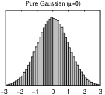
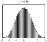
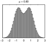
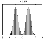
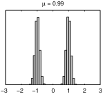
Figure 1: Distribution of coupling constants for the transition from the Gaussian (upper left) to the $\pm J$ spin glass (lower right).

4 Numerical experiments

In the following we describe the numerical experiments in more detail and present results for the spin glasses described above.

4.1 Description of experiments

For $\pm J$ and Gaussian 2D spin glasses, systems with equal number of spins in each dimension were used of size from $n=8\times 8$ to $n=20\times 20$. For each system size, 1000 random samples were generated. hBOA with the deterministic local searcher was then applied to find the ground state for each sample. For the transition from $\pm J$ to Gaussian spin glasses, we focused on a single system size, $n=10\times 10$.

For each spin glass sample, the population size in hBOA is set to the minimum population size required to find the optimum in 10 independent runs. The minimum population size is determined using bisection. The width of the final interval in bisection is at most $10\%$ of its higher limit. Binary tournament selection without replacement is used. The windows size in RTR is set to the number of spins of the system under consideration, but it is always at most equal to $5\%$ of the population size. The $5\%$ cap on the window size is important to ensure fast convergence with even small populations. The cap explains the difference between the results presented here and the previous results, because populations are usually very small for hBOA with local search on Ising spin glasses [8].

Performance of hBOA was measured by (1) $E_{G}$, the total number of spin glass system configurations examined by hBOA (the number of restarts of the local searcher), and (2) $E_{L}$, the total number of steps of the local hill climber. Due to the lack of space, we only analyze $E_{G}$. $E_{L}$ was greater than $E_{G}$ by a factor of approximately $O(\sqrt{n})$. Clearly, we can expect that $E_{G}<E_{L}$. Nonetheless, it is computationally much less expensive to perform a local step in the hill climber than to evaluate a new spin glass configuration sampled by hBOA.

4.2 Results for $\pm J$ and Gaussian couplings

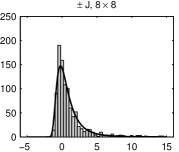
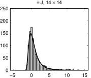
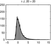
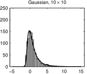
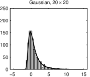
Figure 2: Distribution of $E_{G}$ for $\pm J$ spin glass systems of varying size. $E_{G}$ and the density function are normalized using $\mu$ and $\beta$.

The first important observation is that the distributions of $E_{G}$ and $E_{L}$ for all problem sizes and distributions of coupling constants follow Fréchet extremal value distributions. Applying a maximum likelihood estimator we can determine the parameters $\mu$, $\beta$, and $\xi$ of these distributions defined in Equation (1). Figure 2 shows the histograms and the corresponding probability density function for $E_{G}$ for $\pm J$ spin glasses of various sizes.

The location parameter $\mu$ indicating the most likely value of $E_{G}$ can be used to determine the scalability of hBOA. In Figures 3a and 3b the location parameter for both $\pm J$ and Gaussian spin glasses are shown versus the system size. Double logarithmic plots confirm that the location has an upper polynomial bound. For the $\pm J$ spin glass, the order of that polynomial approaches $1.5$ as system size $n$ grows, whereas for Gaussian couplings, the order of the polynomial seems to approach $2.2$.

Figure 3c and  3d show the shape $\xi$ for both $\pm J$ and Gaussian spin glasses with respect to the system size. Since it is always smaller than 1, we conclude that the mean is well-defined for all cases. For the variance (2nd moment) we find the shape parameter to be smaller than 1/2 only for systems larger than $n=10\times 10$. Thus, for system smaller than $n=10\times 10$ the variance is not well-defined and the mean has an infinite error.

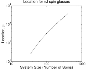
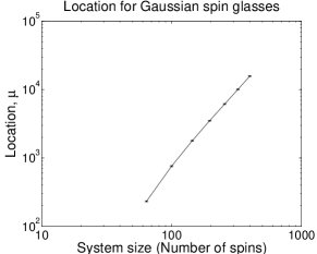
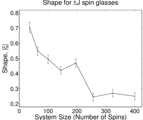
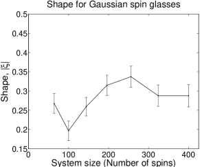
Figure 3: Location $\mu$ and shape $\xi$ for $\pm J$ and Gaussian spin glasses using maximum likelihood estimation. Standard error of the estimations displayed with error bars.

4.3 Results for the transition between $\pm J$ and Gaussian couplings

For the transition between $\pm J$ and Gaussian couplings, $E_{G}$ and $E_{L}$ also follow Fréchet distributions. Figure 4 shows the distribution of $E_{G}$ in the transition, including $\pm J$ and Gaussian cases. Figure 5 shows location and shape parameters for the transition.

We can see that both location and shape parameters for the transition between $\pm J$ and Gaussian couplings lie between the corresponding parameters for the two extreme cases. That means that considering the two extreme cases provides insight not only in the cases themselves, but it can be used to guide estimation of parameters for a large class of other distributions of couplings.

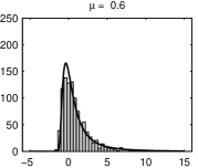
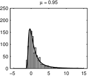
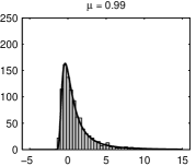
Figure 4: Distribution of $E_{G}$ for the transition from $\pm J$ to Gaussian spin glasses for $n=10\times 10$.

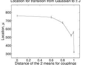
(a) Location

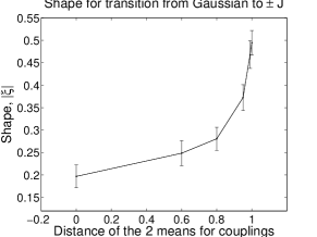
(b) Shape

Figure 5: Location $\mu$ and shape $\xi$ for the transition between $\pm J$ and Gaussian spin glasses. Standard error of the estimations displayed with error bars. X-axis denotes the distance $\tilde{\mu}$ of the means used to generate couplings.

5 Discussion

In the following we discuss the experimental results, first in the context of hBOA scalability theory and then in comparison with flat-histogram Monte Carlo results [13]. We close by presenting some general conclusions for genetic and evolutionary computation.

5.1 Experimental results and hBOA theory

An interesting question is whether the results obtained can be explained using hBOA convergence theory designed for a rather idealized situation, where the problem can be decomposed into subproblems of bounded order over multiple levels of difficulty. For random 2D Ising spin glasses, it can be shown that for a complete single-level decomposition it would be necessary to consider subproblems of order proportional to $\sqrt{n}$ as hypothesized by Mühlenbein  [14], which would lead to exponentially sized populations [15]. Despite this, the number of function evaluations grows as a low-order polynomial of the number $n$ of spins as predicted by hBOA scalability theory for decomposable problems of bounded difficulty [15]. Spin glasses with $\pm J$ couplings correspond to uniform scaling, where the theory predicts $O(n^{1.55})$ evaluations; indeed the location parameter $\mu$ indeed seems to approach a polynomial of order approx. $1.5$. Spin glasses with Gaussian couplings exhibit a non-uniform scaling, where exponential scaling can be taken as a bounding case. For exponential scaling, the number of evaluations would be predicted to grow as $O(n^{2})$; here the location parameter seems to grow slightly faster with a polynomial of order approx. $2.2$. However, the order of this polynomial decreases with problem size.

5.2 Comparison to flat-histogram Monte Carlo

Monte Carlo (MC) methods are usually used to integrate a function $f(x)$ with some probability density distribution over the input parameter $x$. The common approach is to sample a series of values of $x$ according to the specified probability distribution, and averaging the values of $f(x)$.

While conventional MC has been successfully used in numerous applications, it sometimes produces inferior results for low temperatures because the random walk through the space of all possible configurations (values of $x$) of the system has difficulties in overcoming energy barriers. One of the ways to alleviate this difficulty is to modify the simulated statistical-mechanical ensemble and use Wang-Landau sampling [2] to sample each energy level equally likely, thereby producing a flat histogram. The Wang-Landau algorithm thus represents a class of methods also known as flat-histogram MC. This approach not only alleviates the problem of energy barriers, but it also enables computation of the number of configurations at different energy levels, which can in turn be used to quickly compute thermal averages for any given temperature without having to rerun the simulation.

For flat-histogram MC, the distribution of round-trip times in energy measured by the total number of applications of local operators was recently shown to follow Fréchet distributions [13]. However, the absolute value of the shape parameter for flat-histogram MC was shown to approach $1$. As a result, the mean of this distribution is not defined. Further, the location parameter found for flat-histogram MC grows exponentially [13], although for this class of spin glasses it is possible to analytically compute the entire energy spectrum in polynomial time, $O(n^{3.5})$ [11].

5.3 Important lessons for genetic and evolutionary computation

The results presented in this paper indicate that it can be misleading to estimate the mean convergence time by an average over several independent samples (runs), because in some cases the mean, variance, and other moments of the respective distribution may become ill-defined. In this work, the location parameter serves as a well-defined quantity to express computational complexity of various optimization and simulation techniques, including hBOA and flat-histogram MC. It can be expected that similar distribution will be observed for other evolutionary algorithms, as they reflect intrinsic properties of the spin glass [13].

Random 2D Ising spin glasses represent interesting classes of constraint satisfaction problems with a large number of local optima. The results presented in this work indicate that for such classes of problems, recombination-based search can provide optimal solutions in low-order polynomial time, whereas mutation-based methods scale exponentially. However, local search is still beneficial for local improvement of solutions in recombination-based evolutionary algorithms, because incorporating local search decreases population sizing requirements. A similar observation was found for MAXSAT [9].

6 Conclusions

Random classes of Ising spin glass systems represent an interesting class of constraint satisfaction problems for black-box optimization. Similar to flat-histogram MC, computational complexity of hBOA—expressed in the number of solutions explored by both hBOA and the local hill climber until the optimum—is found to show large sample-to-sample variations. The obtained distribution of optimization steps follow a fat-tailed Fréchet extremal value distribution. However, for hBOA the shape parameter defining the decay of the tail is small enough for the first two moments of the observed distributions to exist for all but smallest system sizes. The location parameter as well as the mean of this distribution scale like a polynomial of low order. The experiments show that similar behavior can be observed for $\pm J$ and Gaussian spin glasses, as well as for the transition between these two cases. For $\pm J$ spin glasses, performance of hBOA agrees with scalability theory for hBOA on uniformly scaled problems, whereas for Gaussian spin glasses, performance of hBOA agrees with scalability theory for hBOA on exponentially scaled problems.

There are some general conclusions for genetic and evolutionary computation. First, measuring time complexity by the average number of function evaluations until the optimum is found can sometimes be misleading when rare events dominate the sample-to-sample variations. Second, it was shown for this specific problem that recombination-based search can efficiently deal with exponentially many local optima and still find the global optimum in low-order polynomial time.

References

- [1] Mézard, M., Parisi, G., Virasoro, M.A.: Spin glass theory and beyond. World Scientific, Singapore (1987)
- [2] Wang, F., Landau, D.P.: Efficient, multiple-range random walk algorithm to calculate the density of states. Physical Review Letters 86 (2001) 2050–2053
- [3] Berg, B.A., Neuhaus, T.: Multicanonical ensemble - a new approach to simulate first order phase-transition. Physical Review Letters 68 (1992)
- [4] Pelikan, M., Goldberg, D.E.: Escaping hierarchical traps with competent genetic algorithms. Proceedings of the Genetic and Evolutionary Computation Conference (GECCO-2001) (2001) 511–518 Also IlliGAL Report No. 2000020.
- [5] Pelikan, M., Goldberg, D.E.: A hierarchy machine: Learning to optimize from nature and humans. Complexity 8 (2003)
- [6] Chickering, D.M., Heckerman, D., Meek, C.: A Bayesian approach to learning Bayesian networks with local structure. Technical Report MSR-TR-97-07, Microsoft Research, Redmond, WA (1997)
- [7] Harik, G.R.: Finding multimodal solutions using restricted tournament selection. Proceedings of the International Conference on Genetic Algorithms (ICGA-95) (1995) 24–31
- [8] Pelikan, M.: Bayesian optimization algorithm: From single level to hierarchy. PhD thesis, University of Illinois at Urbana-Champaign, Urbana, IL (2002)
- [9] Pelikan, M., Goldberg, D.E.: Hierarchical boa solves ising spin glasses and maxsat. Proceedings of the Genetic and Evolutionary Computation Conference (GECCO-2003) II (2003) 1275–1286 Also IlliGAL Report No. 2003001.
- [10] Fisher, R.A., Tippett, L.H.C.: Limiting forms of the frequency distribution of the largest and smallest member of a sample. In: Proceedings of Cambridge Philosophical Society. Volume 24. (1928) 180–190
- [11] Galluccio, A., Loebl, M.: A theory of Pfaffian orientations. I. Perfect matchings and permanents. Electronic Journal of Combinatorics 6 (1999) Research Paper 6.
- [12] Galluccio, A., Loebl, M.: A theory of Pfaffian orientations. II. T-joins, k-cuts, and duality of enumeration. Electronic Journal of Combinatorics 6 (1999) Research Paper 7.
- [13] Dayal, P., Trebst, S., Wessel, S., Würtz, D., Troyer, M., Sabhapandit, S., Coppersmith, S.N.: Performance limitations of flat histogram methods. Physical Review Letters (in press)
- [14] Mühlenbein, H., Mahnig, T., Rodriguez, A.O.: Schemata, distributions and graphical models in evolutionary optimization. Journal of Heuristics 5 (1999) 215–247
- [15] Pelikan, M., Sastry, K., Goldberg, D.E.: Scalability of the Bayesian optimization algorithm. International Journal of Approximate Reasoning 31 (2002) 221–258 Also IlliGAL Report No. 2001029.