Surface Triangulation – the Metric Approach

Abstract.

We embark in a program of studying the problem of better approximating surfaces by triangulations(triangular meshes) by considering the approximating triangulations as finite metric spaces and the target smooth surface as their Haussdorff-Gromov limit. This allows us to define in a more natural way the relevant elements, constants and invariants s.a. principal directions and principal values, Gaussian and Mean curvature, etc. By a ”natural way” we mean an intrinsic, discrete, metric definitions as opposed to approximating or paraphrasing the differentiable notions. In this way we hope to circumvent computational errors and, indeed, conceptual ones, that are often inherent to the classical, ”numerical” approach. In this first study we consider the problem of determining the Gaussian curvature of a polyhedral surface, by using the embedding curvature in the sense of Wald (and Menger). We present two modalities of employing these definitions for the computation of Gaussian curvature.

1. Introduction

The paramount importance of triangulations of surfaces and their ubiquity in various implementations (s.a. in numerous algorithms applied in robot (and computer) vision, computer graphics and geometric modelling, with a wide range of applications from industrial ones, to biomedical engineering to cartography and astrography – to number just a few) has hardly to be underlined here. In consequence, determining the intrinsic proprieties of the surfaces under study, and especially computing their Gaussian curvature is essential. However Gaussian curvature is a notion that is defined for smooth surfaces only, and usually attacked with differential tools, tools that – however ingenious and learned – can hardly represent good approximations for curvature of $PL$-surfaces, since they are usually just discretizations of formulas developed in the smooth (i.e. of class at least $\mathcal{C}^{2}$) case.
Moreover, since considering triangulations, one is faced with finite graphs, or, in many cases (when given just the vertices of the triangulation) only with finite –thus discrete – metric spaces. Therefore, the following natural questions arise: (A) Is one fully justified in employing discrete metric spaces when evaluating numerical invariants of continuous surfaces? and (B) Can one find discrete, metric equivalents of the differentiable notions, notions that are intrinsically more apt to describe the properties of the finite spaces under investigations? One is further motivated to ask the questions above, since the metric method we propose to employ have already successfully been used in the such diverse fields as Geometric Group Theory, Geometric Topology and Hyperbolic Manifolds, and Geometric Measure Theory. Their relevance to Computer Graphics in particular and Applied Mathematics in general is made even more poignant by the study of Clouds of Points (see [LWZL], [MD]) and also in applications in Chemistry (see [T]).
We show that the answer to both this questions is affirmative, and we focus our investigations mainly on the study of metric equivalents of the Gauss curvature. Their role is not restricted to that of being yet another discrete version of Gaussian Curvature, but permits us to attach a meaningful notion of curvature to points where the surface fails to be smooth, such as cone points and critical lines. Thus we can employ curvature in reconstructin not only smooth surface, but also surfaces with ”folds”, ”ridges” and ”facets”.
This exposition is organized as follows: in Section 2 we concentrate our efforts on the theoretical level and study the Lipschitz and Gromov-Hausdorff distances between metric spaces, and show that approximating smooth surfaces by nets and triangulations is not only permissible, but is, in a way, the natural thing to do, in particular we show that every compact surface is the Gromov-Hausdorff limit of a sequence of finite graphs. In Section 3 we introduce the best candidate for a metric (discrete) version of the classical Gauss curvature of smooth surfaces, that is the Embedding, or Wald curvature. We study its proprieties and investigate the relationship between the Wald and the Gauss curvatures, and show that for smooth surfaces they coincide, so that the Wald curvature represents a legitimate discrete candidate for approximating the Gaussian curvature of triangulated surfaces. Section 4 is dedicated to developing formulas that allow the computation of Wald curvature: first the precise ones, based upon the Cayley-Menger determinants, and then we develop (after Robinson) elementary formulas that approximate well the Embedding curvature. We conclude with three Appendices. In the first Appendix we present three metric analogues for the curvature of curves, namely the Menger, Alt and Haantjes curvatures and study their mutual relationship. Furthermore we show how to relate to these notions as metric analogues of sectional curvature and how to employ them in the evaluation of Gauss curvature of triangulated surfaces. Next we present yet another metric analogue of surfaces curvature, based, in this case, upon a the modern triangle comparison method, namely the Rinow curvature. We investigate its proprieties and show (following Kirk ([K])) that in the case under investigation the Rinow and Wald curvatures coincide (and therefore Rinow curvature also identifies to the Gauss curvature). The third and last Appendix is dedicated to the development of determinant formula for the radius of the circumscribed sphere around a tetrahedron, with a view towards applications.

2. The Haussdorff-Gromov limits

2.1. Lipschitz Distance

This definition is based upon a very simple idea: it measures the relative difference between metrics, more precisely it evaluates their ratio; i.e.:
The metric spaces $(X,d_{X})$, $(Y,d_{Y})$ are close iff $\exists\;f:X\stackrel{{\scriptstyle\sim}}{{\rightarrow}}Y$ s.t. $\frac{d_{Y}(fx,fy)}{d_{X}(x,y)}\approx\nolinebreak[4]1,\,\\ \forall\ x,y\in X$.
Technically, we give the following:

Definition 2.1.

The map $f:(X,d_{X})\rightarrow(Y,d_{Y})$ is bi-Lipschitz iff $\exists\,c,C>0$ s.t.:

$$c\cdot d_{X}(x,y)\;\leq\;d_{Y}(fx,fy)\;\leq C\;\cdot d_{X}(x,y)\,.$$

Remark 2.2.

The same definition applies for two different metrics $d_{1},d_{2}$ on the same space $X$.

Definition 2.3.

Given a Lipschitz map $f:X\rightarrow Y$, we define the dilatation of f by:

$$dil\,f=\sup_{x\neq y\in X}\frac{d_{Y}(fx,fy)}{d_{X}(x,y)}.$$

Remark 2.4.

The dilatation represents the minimal Lipschitz constant of maps between $X$ and $Y$.

Remark 2.5.

If $f$ is not Lipschitz, then $dil\,f\stackrel{{\scriptstyle\small\triangle}}{{=}}\infty$.

Remark 2.6.

1. $f$ Lipschitz $\Rightarrow$ $f$ continuous.

2. $f$ bi-Lipschitz $\Rightarrow$ $f$ homeo. on its image.

Remark 2.7.

We have the following results:

Proposition 2.8.

Let $f,g:X\rightarrow Y$ be Lipschitz maps. Then:
                          (a) $g\circ f$ is Lipschitz
                      and
                          (b) $dil\,(g\circ f)\leq dil\,f\cdot dil\,g$

Proposition 2.9.

The set $\{f:(X,d)\rightarrow\mathbb{R}\,|\,fLipschitz\}$ is a vector space.

Now we can return to our main interest and define the following notion:

Definition 2.10.

Let $(X,d_{X})$, $(Y,d_{Y})$ be metric spaces. Then the Lipschitz distance between $(X,d_{X})$ and $(Y,d_{Y})$ is defined as:

$$d_{L}(X,Y)=\inf_{\scriptscriptstyle\stackrel{{\scriptstyle f:X\stackrel{{\scriptstyle\sim}}{{\rightarrow}}Y}}{{\tiny f\;bi-Lip.}}}\log{\max{(dil\,f,dil\,f^{-1})}}$$

Remark 2.11.

If $\neq$ $f$ bi-Lipschitz between $X$ and $Y$, then – remembering Remark 2.2 – we put $d_{L}(X,Y)\stackrel{{\scriptstyle\small\triangle}}{{=}}\infty$ (i.e. $d_{L}$ is not suited for pairs of spaces that are not bi-Lipschitz equivalent.)

having defined the distance between two metric spaces we now can define the convergence in this metric in the following natural way:

Definition 2.12.

The sequence of metric spaces $\{(X_{n},d_{n})\}$ convergence to the metric space $\{(X,d)\}$ iff

$$\lim_{n}d_{L}(X_{n},X)=0$$

(In this case we write: $(X_{n},d_{n})\raisebox{-5.69046pt}{$\stackrel{{\scriptstyle\longrightarrow}}{{\scriptstyle L}}$}0$).

Example 2.13.

Let $S_{t}$ be a family of regular surfaces, $S_{t}=f_{t}(U)$; where $U$ is an open set, $U=int\,U\subseteq\mathbb{R}$; such that the family $\{f_{t}\}$ of parametrizations is smooth (i.e. $F:U\times\mathbb{R}\rightarrow\mathbb{R}^{3}\in\mathcal{C}^{1}$; where $F((u,v),t)\stackrel{{\scriptstyle\tiny not}}{{=}}f_{t}(u,v)$). Then $d_{n}(S_{t},S_{0})\raisebox{-4.26773pt}{$\stackrel{{\scriptstyle\longrightarrow}}{{\scriptstyle t\rightarrow 0}}$}\,0$.

Remark 2.14.

If $F$ is not smooth (only continuous) then we do not necessarely have that $S_{t}\raisebox{-4.26773pt}{$\stackrel{{\scriptstyle\longrightarrow}}{{\scriptstyle t\rightarrow 0}}$}S_{0}$ .

We have the following significant theorem:

Theorem 2.15.

The $d_{L}$ satisfies the following conditions:
(a) $d_{L}\geq 0$;
(b) $d_{L}$ is symmetric;
(c) $d_{L}$ satisfies the triangle inequality;
Moreover, if $X,Y$ are compact, then:
(d) $d_{L}(X,Y)=0\Leftrightarrow X\cong Y$ (i.e. $X$ is isometric to $Y$);
that is

$d_{L}$ is a metric on the space of isometry classes of compact metric spaces

Remark 2.16.

Let us recall the following

Definition 2.17.

$(X_{n},d_{n})\raisebox{-4.26773pt}{$\stackrel{{\scriptstyle\longrightarrow}}{{\scriptstyle u}}$}(X,d)\stackrel{{\scriptstyle\small\triangle}}{{=}}\;d_{u}\raisebox{-4.26773pt}{$\stackrel{{\scriptstyle\longrightarrow}}{{\scriptstyle u}}$}\;d$ as a real function; i.e.

$$\sup_{x,y\in X}|d_{n}(x,y)-d(x,y)|\raisebox{-4.26773pt}{$\stackrel{{\scriptstyle\longrightarrow}}{{\scriptstyle u}}$}0$$

(where ”$u$” denotes uniform convergence.)

Then $X_{n}\raisebox{-4.26773pt}{$\stackrel{{\scriptstyle\longrightarrow}}{{\scriptstyle u}}$}X\;\Rightarrow\;X_{n}\raisebox{-4.26773pt}{$\stackrel{{\scriptstyle\longrightarrow}}{{\scriptstyle L}}$}X$ but $X_{n}\raisebox{-4.26773pt}{$\stackrel{{\scriptstyle\longrightarrow}}{{\scriptstyle L}}$}X\Rightarrow{/}\;\;X_{n}\raisebox{-4.26773pt}{$\stackrel{{\scriptstyle\longrightarrow}}{{\scriptstyle u}}$}X$. However, for finite spaces indeed $X_{n}\raisebox{-4.26773pt}{$\stackrel{{\scriptstyle\longrightarrow}}{{\scriptstyle u}}$}X\;\Leftrightarrow\;X_{n}\raisebox{-4.26773pt}{$\stackrel{{\scriptstyle\longrightarrow}}{{\scriptstyle L}}$}X$.

2.2. Gromov-Hausdorff distance

This is also a distance between compact metric spaces ((distinguished) up to isometry!). However it gives a weaker topology (In particular: it is always finite (even for pairs of non-homeomorphic spaces.) )
We start by first introducing the classical

2.2.1. Hausdorff distance

Definition 2.18.

Let $A,B\subseteq(X,d)$. We define the Hausdorff distance between $A$ and $B$ as:

$$d_{H}(A,B)=\inf\{r>0\,|\,A\subset U_{r}(B),\,B\subset U_{r}(A)\}$$

(see Fig. 1);

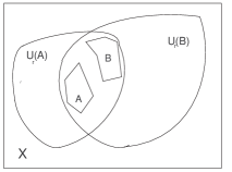
Figure 1.

where $U_{r}(A)$ is the $r$-neighborhood of A, $U_{r}(A)\stackrel{{\scriptstyle\scriptstyle\triangle}}{{=}}\bigcup_{a\in A}B_{r}(a)$; (here, as usual: $B_{r}(a)=\{x\in X\,|\,d(a,x)<r\}$.)

Another (equivalent) way of defining the Hausdorff distance is as follows:

$$d_{H}(A,B)=\max\{\sup_{a\in A}d(a,B),\,\sup_{b\in B}d(b,A)\}\,.$$

(see Fig. 2)

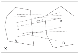
Figure 2.

We have the following

Proposition 2.19.

Let $(X,d)$ be a metric space. Then:
(a) $d_{H}$ is a semi-metric (on $2^{X}$). (i.e. $A=B\Rightarrow d_{H}{(A,B)}=0$.)
(b) $d_{H}(A,\bar{A})=0,\forall A\subseteq X$.
(c) $\big{(}A=\bar{A}\;and\;B=\bar{B}\big{)}\Rightarrow\big{(}d_{H}(A,B)=0\Leftrightarrow A=B\big{)}$.
i.e. $d_{H}$ is a metric on the set of closed subsets of X.

Notation We put: $\mathcal{M}(X)=\big{(}\{A\subseteq X\,|\,A=\bar{A}\},d_{H}\big{)}=2^{X}/d_{H}$ .

Remark 2.20.

1. if $X$ is compact and if $\{A_{n}\}_{n\geq 1}\subseteq X$ is a sequence of compact subsets of $X$, then:

   1. $A_{n+1}\subseteq A_{n}\Rightarrow A_{n}\raisebox{-4.26773pt}{$\stackrel{{\scriptstyle\longrightarrow}}{{\scriptstyle H}}$}\bigcap_{n\geq 1}A_{n}$ .
      

   2. $A_{n}\subseteq A_{n+1}\Rightarrow A_{n}\raisebox{-4.26773pt}{$\stackrel{{\scriptstyle\longrightarrow}}{{\scriptstyle H}}$}\bigcup_{n\geq 1}A_{n}$ .
      

2. For general subsets $A_{n}\raisebox{-4.26773pt}{$\stackrel{{\scriptstyle\longrightarrow}}{{\scriptstyle H}}$}A\in\mathcal{M}(X)$ , and
   

   1. $A=\{\lim_{n}a_{n}\,|\,a_{n}\in A_{n}\,;n\geq 1\}$ .
      

   2. $A=\raisebox{-4.26773pt}{$\stackrel{{\scriptstyle\longrightarrow}}{{\scriptstyle H}}$}\bigcap_{n\geq 1}\big{(}\overline{\bigcup_{m=n}^{\infty}A_{m}}\big{)}$ .

3. If $A_{n}\raisebox{-4.26773pt}{$\stackrel{{\scriptstyle\longrightarrow}}{{\scriptstyle H}}$}A$, and if the sets $A_{n}$ are all convex, then $A$ is convex sets.

We have the following two important results, which we present without their respective (lengthy) proofs:

Proposition 2.21.

$X$ complete $\Rightarrow\;\mathcal{M}(X)$ complete .

Theorem 2.22.

​(Blaschke)  $X$ compact $\Rightarrow\;\mathcal{M}(X)$ compact .

2.3. The Gromov-Hausdorff Distance

We are now able to define the Gromov-Hausdorff distance using the following basic guide-lines: we want to get the maximum distance that satisfies the following two conditions:
(a) $d_{GH}(A,B)\leq d_{H}(A,B),\forall A,B\subset X$ (i.e. set that are close as subsets of $X$ will still be close as abstract metric spaces);
and
(b) $X$ isometric to $Y$ $\Longleftrightarrow$ $d_{GH}(X,Y)=0$.

Definition 2.23.

Let $X,Y$ be metric spaces. Then the Gromov-Hausdorff distance between $X$ and $Y$ is defined by:

$$d_{GH}(X,Y)\stackrel{{\scriptstyle\scriptstyle\triangle}}{{=}}\inf d_{H}^{Z}(f(X),g(Y))$$

where the infimum is taken over all the isometric embeddings $f:X\hookrightarrow Z,g:Y\hookrightarrow Z$ into some metric space Z. (See Fig. 3).

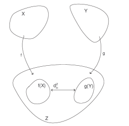
Figure 3.

Remark 2.24.

If $X=\mathbb{S}^{2}$, with the spherical metric, and $Z=\mathbb{R}^{3}$, with the Euclidian metric, then $f(X)\neq X$ (!)

Example 2.25.

Let $Y$ be an $\varepsilon$-net in $X$. Then $d_{GH}(X,Y)\leq\varepsilon$.
Proof Take $Z=X=X^{\prime}\,,\;Y=Y^{\prime}$.
$\Box$

Remark 2.26.

It is sufficient to consider embeddings $f$ into the disjoint union of the spaces $X$ and $Y$, $X\coprod Y$.

Remark 2.27.

1. $X,Y$ bounded $\Longrightarrow$ $d_{GH}(X,Y)\leq\infty$.
   

2. If $diamX,diamY<\infty$, then $d_{GH}(X,Y)\geq\frac{1}{2}|diamX-diamY|$.

However , the straightforward definition of $d_{GH}$ may be difficult to implement. Therefore we would like to estimate (compute) $d_{GH}$ by comparing distances in $X$ vs. distances in $Y$ (as done in the cases of uniform and Lipschitz metrics). We start by defining a correspondence between metric spaces: $X\longleftrightarrow Y$, given by correspondences $x\leftrightarrow y$ between points $x\in X,y\in Y$.

Remark 2.28.

A correspondence is not necessarely a function, that is to a single $x$ may correspond to several $y$-’s.

We shall prove that

$$(*)\>\>\>\>d_{GH}(X,Y)<r\;\Longleftrightarrow\;\exists\;a\;correspondenceX\longleftrightarrow Y\;$$

$$\hskip 128.0374pts.t.\;(x\leftrightarrow y,x^{\prime}\leftrightarrow y^{\prime})\;\Longrightarrow\;|d_{X}(x,x^{\prime})-d_{Y}(y,y^{\prime})|<2r$$

Formally, we have:

Definition 2.29.

Let $X,Y$ denote sets. A correspondence $X\longleftrightarrow Y$ is a subset of the Cartesian product of $X$ and $Y$: $\mathcal{R}\subset X\times Y$ s.t.
(i) $\forall x\in X,\exists y\in Y,s.t.(x,y)\in\mathcal{R}$;
and
(ii) $\forall y\in Y,\exists x\in X,s.t.(x,y)\in\mathcal{R}$.

Example 2.30.

Any surjective function $f:X\rightarrow Y$ represents correspondence
$\mathcal{R}=\{(x,f(x))\}$.

Remark 2.31.

$\mathcal{R}$ is a correspondence $\Longleftrightarrow$ $\exists\;Z$ and $\exists\;f:Z\rightarrow X\,,\exists g:Z\rightarrow Y$; $f,g$ surjective, s.t. $\mathcal{R}=\{(f(z),g(z))\,|\,z\in Z\}$.

Definition 2.32.

Let $\mathcal{R}$ be a correspondence between $X$ and $Y$, where $X,Y$ are metric spaces. We Define the distortion of $\mathcal{R}$ by:

$$dis\,\mathcal{R}=\sup\big{\{}\,|d_{X}(x,x^{\prime})-d_{Y}(y,y^{\prime})|\,\big{|}\,(x,y)\,,(x^{\prime},y^{\prime})\in\mathcal{R}\big{\}}\,.$$

(See (*) .)

Remark 2.33.

1. If $\mathcal{R}=\{(x,f(x))\}$ is a correspondence induced by a surjective function $f:X\rightarrow Y$, then $dis\,\mathcal{R}=dis\,f$, where:

   $$dis\,f\stackrel{{\scriptstyle\scriptstyle\triangle}}{{=}}\sup_{a,b\in X}|\,d_{Y}(fa,fb)-d_{X}(a,b)\,|\,.$$

2. If $\mathcal{R}=\{(f(z),g(z))\}$, where $f:X\rightarrow Z,\;g:Y\rightarrow Z$ are surjective functions, then:

   $$dis\,\mathcal{R}=\sup_{z,z^{\prime}\in Z}\{\,|\,d_{X}(fz,fz^{\prime})-d_{Y}(gz,gz^{\prime})\,|\,\}\,.$$

3. $\mathcal{R}=0$ iff $\mathcal{R}$ is associated to an isometry.

We bring, without proof, the following theorem:

Theorem 2.34.

Let $X,Y$ be metric spaces. Then:

$$d_{GH}(X,Y)=\frac{1}{2}\inf_{{\tiny\mathcal{R}}}(dis\,\mathcal{R})\,;$$

where the infimum is taken over all the correspondences $X\stackrel{{\scriptstyle\mathcal{R}}}{{\longleftrightarrow}}Y$.

Before bringing the next result (which is very important in determining the topology ) we first introduce one more notion:

Definition 2.35.

$f:X\rightarrow Y$ is called an $\varepsilon$-isometry ($\varepsilon>0$), iff
(i) $dis\,f\leq\varepsilon$,
and
(ii) $f(x)$ is an $\varepsilon$-net in $Y$.

Remark 2.36.

$f\;\varepsilon$-isometry $\Longrightarrow/$    $f$ continuous.

Corollary 2.37.

Let $X,Y$ be metric spaces and let $\varepsilon>0$. Then:
(i) $d_{GH}(X,Y)<\varepsilon\Longrightarrow\exists\;2\varepsilon{-isometry}\;f:X\rightarrow Y$.
(ii) $\exists\;\varepsilon{-isometry}\;f:X\rightarrow Y\Longrightarrow d_{GH}(X,Y)<2\varepsilon$.

Proof (i) Let $X\stackrel{{\scriptstyle\mathcal{R}}}{{\longleftrightarrow}}Y$ s.t. $dis\,\mathcal{R}<2\varepsilon$.
For any $x\in X$ and $f(x)\in Y$, choose $y=f(x)$ s.t. $(x,f(x))\in\mathcal{R}$. Then $x\mapsto f(x)$ defines a map $f:X\rightarrow Y$. Moreover: $dil\,f\leq dil\,\mathcal{R}<\varepsilon$.
We shall prove that $f(X)$ is a $2\varepsilon$-net in $Y$.
Indeed, let $x\in X$ and $y\in Y$ s.t. $(x,y)\in\mathcal{R}$. Then $d(y,fx)\leq d(x,x)+dis\,\mathcal{R}<2r$, thence $d(y,f(X))<2r$.
                                                                                               $\square$
Let $f$ be an $2\varepsilon$-isometry. Define $\mathcal{R}\subset X\times Y,\;\mathcal{R}=\{(x,y)\,|\,d(y,fx)\leq\varepsilon\}$.
Then, since $f(X)$ is an $\varepsilon$-net it follows that $\mathcal{R}$ is a correspondence.
Then $\forall\,(x,y),(x^{\prime},y^{\prime})\in\mathcal{R}$ we have:

$$|\,d_{Y}(y,y^{\prime})-d_{X}(x,x^{\prime})\,|\leq|\,d(fx,fx^{\prime})-d(x,x^{\prime})\,|+d(y,fx)+d(y^{\prime},fx^{\prime})\leq dis\,f+\varepsilon+\varepsilon\leq 3\varepsilon\,.$$

$$\Longrightarrow dis\,\mathcal{R}\leq 3\varepsilon\;\Longrightarrow\;d_{GH}(x,y)\leq 3r/2<2r\,.$$

$\square$
The next result is of great importance (in particular so in our context):

Theorem 2.38.

$d_{GH}$ is a (finite) metric on the set of isometry classes of compact metric spaces.

Proof It suffices to prove that $d_{GH}(X,Y)=0\Longrightarrow X\stackrel{{\scriptstyle\sim}}{{\equiv}}Y$.
Indeed, let $X,Y$ be compact spaces s.t. $d_{GH}=0$. Then it follows from the previous Corollary (for $\varepsilon=1/n$) that $\exists\;(f_{n})_{n\geq 1},\,f_{n}:X\rightarrow Y$ s.t. $dis\,f_{n}\raisebox{-3.00003pt}{$\stackrel{{\scriptstyle\longrightarrow}}{{\scriptstyle n}}$}0$.
let $S\subset X,\;\bar{S}\,,\;|S|=\aleph_{0}$. Using a Cantor-diagonal argument one easily shows that $\exists\;(f_{n_{k}})_{k\geq 1}\subset(f_{n})_{n\geq 1}$ s.t. $(f_{n_{k}})_{\geq 1}$ converges in $Y,\forall x\in S$. Without restricting the generality we may assume that this happens for $(f_{n})_{n\geq 1}$ itself. Thus we can define a function $f:X\rightarrow Y$ by putting: $f(x)=\lim_{n}f_{n}(x)$.
But $|\,d(f_{n}x,f_{n}y)-d(x,y)\,|\leq dis\,f_{n}\raisebox{-3.00003pt}{$\stackrel{{\scriptstyle\longrightarrow}}{{\scriptstyle n}}$}0\;\Longrightarrow\;d(fx,fy)=\lim d(f_{n}x,f_{n}y)$. In other words $f|\raisebox{-1.99997pt}{$S$}$ is an isometry. But $S=\bar{S}$, therefore this isometry can be extended to an isometry $\tilde{f}$ from $X$ to $Y$. In a analogous manner one shows the existence of an isometry $\tilde{\tilde{f}}:X\rightarrow Y$.
$\Box$

Remark 2.39.

$X_{n}\raisebox{-3.99994pt}{$\stackrel{{\scriptstyle\longrightarrow}}{{\scriptstyle L}}$}X\;\Longrightarrow\;X_{n}\raisebox{-3.00003pt}{$\stackrel{{\scriptstyle\longrightarrow}}{{\scriptstyle u}}$}X\;\Longrightarrow\;X_{n}\raisebox{-3.99994pt}{$\stackrel{{\scriptstyle\longrightarrow}}{{\scriptstyle GH}}$}X$.

In fact, the following relationship exists between ”$\stackrel{{\scriptstyle\longrightarrow}}{{\scriptstyle L}}$” and ”$\stackrel{{\scriptstyle\longrightarrow}}{{\scriptstyle GH}}$”:

Theorem 2.40.

$X_{n}\raisebox{-5.0pt}{$\stackrel{{\scriptstyle\longrightarrow}}{{\scriptstyle GH}}$}X\;\Longleftrightarrow\;\;\varepsilon$-nets in $X_{n}\raisebox{-5.0pt}{$\stackrel{{\scriptstyle\longrightarrow}}{{\scriptstyle L}}$}\varepsilon$-nets in $X$.

One can formulate this assertion in a more formal manner and it directly (see [G+], pg. 73). However we shall proceed in more ”delicate” manner, starting with:

Definition 2.41.

Let $X,Y$ be compact metric spaces, and let $\varepsilon,\delta>0$. $X,Y$ are called $\varepsilon$-$\delta$-approximations (of each-other) iff: $\exists$ $\{x_{i}\}_{i=1}^{N}\subset X$, $\exists$ $\{y_{i}\}_{i=1}^{N}\subset Y$ s.t.
(i) $\{x_{i}\}_{i=1}^{N}$ is an $\varepsilon$-net in $X$ and $\{y_{i}\}_{i=1}^{N}$ is an $\varepsilon$-net in $Y$;
(ii) $|\,d_{X}(x_{i},x_{j})-d_{(}y_{i},y_{j})\,|<\delta\;\forall\,i,j\in\{1,...,N\}$.
An $(\varepsilon,\varepsilon)$-approximation is called, for short: an $\varepsilon$-approximation.

The relationship between this last definition and the Gromov-Hausdorff distance is first revealed in

Proposition 2.42.

Let $X,Y$ be compact metric spaces. Then:

1. If $Y$ is a $(\varepsilon,\delta)$-approximation of $X$, then $d_{GH}(X,Y)<2\varepsilon+\delta$.

2. $d_{GH}(X,Y)<\varepsilon\;\Longrightarrow\;Y$ is a $5\varepsilon$-approximation of $X$.

Proof (1) Condition (ii) of Def. 2.41. is equivalent to $dis\,\mathcal{R}_{X_{0}Y_{0}}<\delta$, where
$X_{0}=\{x_{i}\}_{i=1}^{N}\,,\{y_{i}\}_{i=1}^{N}$. But $dis\,\mathcal{R}_{X_{0}Y_{0}}<\delta\;\Longrightarrow\;d_{GH}(X_{0},Y_{0})<\delta/2$. Now, since $X_{0}$ and $Y_{0}$ are $\varepsilon$-nets in $X$, resp. $Y$, it follows that $d_{GH}(X,X_{0})\leq\varepsilon,d_{GH}(Y,Y_{0})<\varepsilon$. From here and from the $d_{GH}(X_{0},Y_{0})<\delta/2$ follows, by means of he triangle inequality, that $d_{GH}(X,Y)<2\varepsilon+\delta$.
                                                                                                          $\square$
(2) By Cor. 2.37., there exists a $2\varepsilon$-isometrie $f:X\rightarrow Y$. Let $X_{0}=\{x_{i}\}_{i=1}^{N}$ be an $\varepsilon$-net, and let $y_{i}=f(x_{i})$.
Then $|\,d(x_{i},x_{j})-d_{(}y_{i},y_{j})\,|<2\varepsilon<5\varepsilon$. Therefore suffice to prove that $Y_{0}=\{y_{i}\}_{i=1}^{N}$ is a $5\varepsilon$-net in $Y$.
Indeed, if $y\in Y$, then, since $f(X)$ is an $2\varepsilon$-net in $Y$, $\exists\,x\in X$ s.t. $d(y,f(x))$. Now, since $X_{0}$ is an $\varepsilon$-net in $X$, $\exists x_{i}\in X_{0}$, s.t. $d(x,x_{i})\leq\varepsilon$.
Therefore: $d(y,y_{i})=d(y,f(x_{i}))\leq d(y,f(x))+d(f(x),f(x_{i}))$
                                           $\leq 2\varepsilon+d(x,x_{i})+dis\,f$
                                           $\leq 2\varepsilon+\varepsilon+2\varepsilon\leq 5\varepsilon$.
$\Box$

Remark 2.43.

Prop. 2.42. $\Longleftrightarrow$ $(X_{n}\raisebox{-5.0pt}{$\stackrel{{\scriptstyle\longrightarrow}}{{\scriptstyle GH}}$}X)$ $\Leftrightarrow$ ($\forall\,\varepsilon>0,\;X_{n}$ is an $\varepsilon$-approximation,                                                                            $\forall\,n$ large enough.)

More precisely we have the following Proposition:

Proposition 2.44.

Let $X,\{X_{n}\}_{1}^{\infty}$ compact metric spaces. Then:
$X_{n}\raisebox{-5.0pt}{$\stackrel{{\scriptstyle\longrightarrow}}{{\scriptstyle GH}}$}X$ $\Longleftrightarrow$ $\forall\varepsilon>0,\;\exists$ a finite $\varepsilon$-net $S\subset X$ and $\exists$ a finite $\varepsilon$-net $S_{n}\subset X_{n}$, s.t. $S_{n}\raisebox{-5.0pt}{$\stackrel{{\scriptstyle\longrightarrow}}{{\scriptstyle GH}}$}S$ and, moreover, $|S_{n}|=|S|$, for large enough $n$.

Proof ($\Longleftarrow$) If $S,S_{n}$ exist, then $\Longrightarrow\;X_{n}$ is an $\varepsilon$-approximation of $X$ $\stackrel{{\scriptstyle 2.42.}}{{\Longrightarrow}}\;X_{n}\raisebox{-5.0pt}{$\stackrel{{\scriptstyle\longrightarrow}}{{\scriptstyle GH}}$}X$ $\forall\,n$.
                                                    
                                                                                                          $\square$
         ($\Longrightarrow$) Let $S$ be an finite $\varepsilon/2$-net in $X$.
We construct in $X_{n}$ corresponding nets $S_{n}$ (to be more precise, we define: $S_{n}=f_{n}(X)$, where $f_{n}$ is an $\varepsilon_{n}$-approximation, $f_{n}:X\rightarrow X_{n},\;\varepsilon_{n}\rightarrow 0$.) Then $S_{n}\raisebox{-5.0pt}{$\stackrel{{\scriptstyle\longrightarrow}}{{\scriptstyle GH}}$}S$ and, in addition, $S_{n}$ is an $\varepsilon$-net in $S$ (for $n$ large enough).
$\Box$

We make the following extremely important Remark:

Remark 2.45.

Let $\mathcal{M}(n,k,D)$ be an $n$-dimensional manifold, of (sectional, Ricci) curvature $\leq k$, and s.t. $diam\,\mathcal{M}\geq D$. Then $(\mathcal{M},d_{GH})$ is compact. However, it should be noted that this result doesn’t hold for curvature $<k$. (only for $Vol(\mathcal{M})\leq V_{0})$ and injectivity radius $\geq r_{0}$.

Note With the notations of the precedent Proposition, the distances in $S_{n}$ converge to the distances in $S$, as $X_{n}\raisebox{-5.0pt}{$\stackrel{{\scriptstyle\longrightarrow}}{{\scriptstyle GH}}$}X$, therefore The Geometric Proprieties of $S_{n}$ will converge to those of $S$. Thus we can use the Gromov-Hausdorff each and every time The Geometric Proprieties of $X_{n}$ can be expressed in term of a finite number of points, and, by passing to the limit, automatically obtain proprieties of $X$.
A typical example is that of the intrinsic metric i.e. the metric induced by a length structure (i.e. path length) by a metric on a subset (of a given metric space). (See Fig. 4 for the classical example of surfaces in $\mathbb{R}^{3}$.)

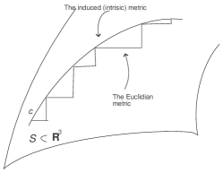
Figure 4.

On a more formal note, we have the following characterization of intrinsic metrics:

Theorem 2.46.

Let $(X,d)$ be a complete metric space.

1. If $\forall\,x,y\in X,\;\exists\frac{1}{2}xy$, then $d$ is strictly intrinsic.

2. If $\forall\,x,y\in X$ and $\forall\varepsilon>0,\;\exists$ the $\varepsilon$-middle of $xy$, then $d$ is intrinsic.

Where we used the following definitions and notations:

Definition 2.47.

1. Given $x,y$ points in $(X,d)$, the middle (or midpoint) of the segment $xy$ (more correctly: ’a midpoint between ”$x$” and ”$y$” ’) is defined as:

   $$\frac{1}{2}xy=z,\;d(x,z)=d(z,y)\,.$$

2. $d$ is called strictly intrinsic iff the length structure is associated with is complete.

3. Let $d$ be an intrinsic metric. $z$ is an $\varepsilon$-middle (or an $\varepsilon$-midpoit) for $xy$ iff:
   $|\,2d(x,z)-d(x,y)\,|\leq\varepsilon$ and $|\,2d(y,z)-d(x,y)\,|\leq\varepsilon$.

Remark 2.48.

The converse of Thm. 2.46. holds in any metric space, more precisely we have:

Proposition 2.49.

If $d$ is an intrinsic metric, then $\frac{1}{2}xy$ exists, $\forall x,y$.

The following Theorem shows that length spaces are closed in the GH-topology :

Theorem 2.50.

Let $\{X_{n}\}$ be length spaces and let $X$ be a complete metric space                         s.t. $X_{n}\raisebox{-5.0pt}{$\stackrel{{\scriptstyle\longrightarrow}}{{\scriptstyle GH}}$}X$.
                       Then $X$ is a length space.

Proof We have already presented the idea of the proof: it is sufficient to show that for every $x,y$ there exist an $\varepsilon$-midpoit ($\forall\varepsilon>0$).
Indeed, let $n$ be such that $d_{GH}<\frac{\varepsilon}{10}$. Then, from the a preceding result, it follows that there exist a correspondence $X_{n}\raisebox{-1.00006pt}{$\stackrel{{\scriptstyle\scriptstyle\mathcal{R}}}{{\longleftrightarrow}}$}X$ s.t. $dis\,\mathcal{R}<\frac{\varepsilon}{5}$.
Let $\bar{x},\bar{y}\in X_{n}$, $x\raisebox{-1.00006pt}{$\stackrel{{\scriptstyle\scriptstyle\mathcal{R}}}{{\leftrightarrow}}$}\bar{x}$, $y\raisebox{-1.00006pt}{$\stackrel{{\scriptstyle\scriptstyle\mathcal{R}}}{{\leftrightarrow}}$}\bar{y}$. Since $X_{n}$ is a length space, $\Longrightarrow\exists\bar{z}\in X_{n}$ s.t. $\bar{z}=\frac{\varepsilon}{5}$-midpoint of $x_{n}y_{n}$. Consider $z\in X,\;z\raisebox{-1.00006pt}{$\stackrel{{\scriptstyle\scriptstyle\mathcal{R}}}{{\leftrightarrow}}$}\bar{z}$. Then:

$$\big{|}|xz|-\frac{1}{2}|xy|\big{|}\leq\big{|}|\bar{x}\bar{z}|-\frac{1}{2}|\bar{x}\bar{y}|\big{|}+2dis\,\mathcal{R}<\frac{\varepsilon}{5}+\frac{2\varepsilon}{5}<\varepsilon\,.$$

(Here we write $|xy|$ instead of $d(x,y)$, etc.)
In a similar manner we show that: $\big{|}|yz|-\frac{1}{2}|xy|\big{|}<\varepsilon$; i.e. $\varepsilon$-midpoit of $xy$.
$\Box$

The next Theorem and its Corollary are of paramount importance:

Theorem 2.51.

Any compact length space is the GH-limit of a sequence of finite graphs.

Proof Let $\varepsilon,\delta\;(\delta\ll\varepsilon)$ small enough, and let $S$ be a $\delta$-net in $X$.
Let $G=(V,E)$ be the graph with $V=S$ and $E=\{(x,y)\,|\,d(x,y)<\varepsilon\}$. we shall prove that $G$ is an $\varepsilon$-approximation of $X$, for $\delta$ small enough (i.e. for $\delta<\frac{\varepsilon^{2}}{4}\,diam(X)$). (See Fig. 5.)

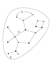
Figure 5.

But, since $S$ is an $\varepsilon$-net both in $X$ and in $G$, and since $d_{G}(x,y)\geq d_{X}(x,y)$, it is sufficient to prove that:

$$d_{G}(x,y)\leq d_{X}(x,y)+\varepsilon\,.$$

Let $\gamma$ be the shortest path between $x$ and $y$, and let $x_{1},...,x_{n}\in\gamma$ s.t. $n\leq length(\gamma)/\varepsilon$ (and $|x_{i},x_{i+1})|\leq\varepsilon/2)$. Since $\forall\,x_{i}\,\exists y_{i}\in S$ s.t. $|x_{i},y_{i}|\leq\delta$, it follows that $|y_{i}y_{i+1}|\leq|x_{i}x_{i+1}|+2\delta<\varepsilon.$ (See Fig. 6)
Therefore, (for $\delta<\varepsilon/4$) $\exists$ an edge $e\in G,e=y_{i}y_{i+1}$. From this we get the following upper bound for $d_{G}(x,y)$:

$$d_{G}(x,y)\leq\Sigma_{0}^{n}|y_{i}y_{i+1}|\leq\Sigma_{0}^{n}|x_{i}x_{i+1}|+2\delta n$$

But $n<2length(\gamma)/\varepsilon\leq 2diam(X)/\varepsilon$; therefore:

$$d_{G}(x,y)\leq|xy|+\delta\frac{4diam(X)}{\varepsilon}<|xy|+\varepsilon\,.$$

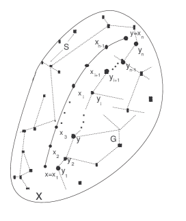
Figure 6.

(because $\delta<\varepsilon^{2}/4diam(X)$).
So, for any $\varepsilon>0,\;\exists\,G=G_{\varepsilon}$ an $\varepsilon$-approximation of $X$. Then, $G_{n}\raisebox{-3.00003pt}{$\stackrel{{\scriptstyle\rightarrow}}{{\scriptstyle\varepsilon}}$}X$.
$\Box$

Corollary 2.52.

Let $X$ be a compact length space. Then $X$ is the Gromov-Hausdorff limit of a sequence $\{G_{n}\}_{n\geq 1}$ of finite graphs, isometrically embedded in $X$.

Remark 2.53.

1. If $G_{n}\raisebox{-3.00003pt}{$\stackrel{{\scriptstyle\rightarrow}}{{\scriptstyle\varepsilon}}$}X$, $G_{n}=(V_{n},E_{n})$. If $\exists N_{0}\in\mathbb{N}$ s.t.

   $$(\star)\;\;\;|E_{n}|\leq N_{0},\;\forall n\in\mathbb{N}\,,$$

   then $X$ is a finite graph.

2. If condition $(\star)$ is replaced by:

   $$(\star\star)\;\;\;|V_{n}|\leq N_{0},\;\forall n\in\mathbb{N}\,,$$

   then $X$ will still be always a graph, but not necessarily finite(!)

3. The Embedding Curvature

3.1. Theoretical Setting

This is basically a comparison-curvature (as is the more ”modern” $CAT$ approach). This is done with quadruples instead of triangles (like in the Alexandrov-Topogonov method). It is in a sense a more natural idea, since quadruples are classically the ”minimal” geometric figures that allow the differentiation between metric spaces. This allows for a much more easier and rapid development of the theory than the triangle-based comparison. Moreover we shall show that the two Theories coincide on those metric space on which both can be applied, i.e. metric spaces that are (a) ”planar” and (b) ”rich enough” i.e. contain quadrangles, s.a. classical (PL-smooth) surfaces in $\mathbb{R}^{3}$.

Definition 3.1.

Let $(M,d)$ be a metric space, and let $Q=\{p_{1},...,p_{4}\}\subset M$, together with the mutual distances: $d_{ij}=d_{ji}=d(p_{i},p_{j});\,1\leq i,j\leq 4$. The set $Q$ together with the set of distances $\{d_{ij}\}_{1\leq i,j\leq 4}$ is called a metric quadruple.

Remark 3.2.

One can define metric quadruples in slightly more abstract manner, without the aid of the ambient space: a metric quadruple being a $4$ point metric space; i.e. $Q=\big{(}\{p_{1},...,p_{4}\},\{d_{ij}\}\big{)}$, where the distances $d_{ij}$ verify the axioms for a metric.

Before we proceed to the next definition, let us introduce the following

Notation $S_{\kappa}$ denotes the complete, simply connected surface of constant curvature $\kappa$, i.e. $S_{\kappa}\equiv\mathbb{R}^{2}$, if $\kappa=0$; $S_{\kappa}\equiv\mathbb{S}^{2}_{\sqrt{\kappa}}$ , if $\kappa>0$; and $S_{\kappa}\equiv\mathbb{H}^{2}_{\sqrt{-\kappa}}$  , if $\kappa<0$. Here $S_{\kappa}\equiv\mathbb{S}^{2}_{\sqrt{\kappa}}$ denotes the Sphere of radius $R=1/\sqrt{\kappa}$, and $S_{\kappa}\equiv\mathbb{H}^{2}_{\sqrt{-\kappa}}$ stands for the Hyperbolic Plane of curvature $\sqrt{-\kappa}$, as represented by the Poincare Model of the plane disk of radius $R=1/\sqrt{-\kappa}$

Definition 3.3.

The embedding curvature $\kappa(Q)$ of the metric quadruple $Q$ is defined be the curvature $\kappa$ of $S_{\kappa}$ into which $Q$ can be isometrically embedded. (See Figures 7 and 8 for embeddings of the metric quadruple in $S_{\kappa}$ and $H_{\kappa}$, respectively.)

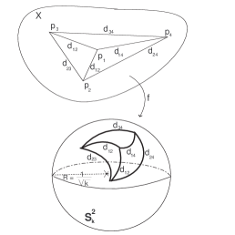
Figure 7.

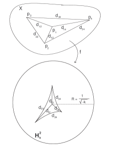
Figure 8.

We can now define the embedding curvature at a point in a natural way by passing to the limit (but without neglecting the existence conditions), more precisely:

Definition 3.4.

Let $(M,d)$ be a metric space, and let $p\in M$ be an accumulation point. Then $p$ is said to have Wald curvature $\kappa_{W}(p)$ iff
(i) $\exists/\,\,N\in\mathcal{N}(p),N$ linear ;
(ii) $\forall\,\varepsilon>0,\;\exists\,\delta>0$ s.t. $Q=\{p_{1},...,p_{4}\}\subset M\,,$ and s.t. $d(p,p_{i})<\delta\,(i=1,...,4)$
$\Longrightarrow|\kappa(Q)-\kappa_{W}(p)|<\varepsilon$.

Remark 3.5.

1. If one uses the second (abstract) definition of the metric curvature of quadruples, then the very existence of $\kappa(Q)$ is not assured, as it is shown by the following

   Counterexample 3.6.

   The metric quadruple of lengths

   $$d_{12}=d_{13}=d_{14}=1;\;d_{23}=d_{24}=d_{34}=2$$

   admits no embedding curvature.

2. Even if a quadruple has an embedding curvature, it still may be not unique (even if $Q$ is not liniar), indeed, one can study the following examples:

   Example 3.7.

   1. The quadruple $Q$ of distances $d_{ij}=\pi/2,1\leq i<j\leq 4$ is isometrically embeddable both in $S_{0}=\mathbb{R}^{2}$ and in $S_{1}=\mathbb{S}^{2}$.

   2. The quadruple $Q$ of distances $d_{13}=d_{14}=d_{23}=d_{24}=\pi,\;d_{12}=d_{34}=3\pi/2$ admits exactly two embedding curvatures: $\kappa_{1}\in(1.5,2)$ and $\kappa_{2}=3$. (See [BM].)

However, for ”good” metric spaces the embedding curvature exists and it is unique. And, what is even more relevant for us, this embedding curvature coincides with the classical Gaussian curvature. The proof of this result is rather long and tedious, therefore we shall present here only a brief sketch of it. (This will prove to be somewhat redundant anyhow, in view of the more general results presented in the previous section, a fact but we shall emphasize later in our presentation).)
The Main ingredient for this proof, and for the analysis of yet another another approach to curvature (the CAT one) is provided by the following string of propositions (which are just generalizations of the well known high-school triangle inequalities):

Proposition 3.8.

Let $\triangle(p_{1},q_{1},r_{1})\subset\mathcal{S}_{\kappa_{1}}$ and $\triangle(p_{2},q_{2},r_{2})\subset\mathcal{S}_{\kappa_{2}}$, s.t.
$p_{1}q_{1}=p_{2}q_{2},\;p_{1}r_{1}=p_{2}r_{2}$ and $\angle(q_{1},p_{1},r_{1})=\angle(q_{2},p_{2},r_{2})$.
Then: $\kappa_{1}<\kappa_{2}\Longrightarrow q_{1}r_{1}>q_{2}r_{2}$.

Proposition 3.9.

Let $p_{1},q_{1},r_{1}\in\mathcal{S}_{\kappa_{1}},\;p_{2},q_{2},r_{2}\in\mathcal{S}_{\kappa_{2}}$ two isometric triples of points, s.t. the triple $p_{1},q_{1},r_{1}$is not linear. Then:
$\angle(q_{1},p_{1},r_{1})<\angle(q_{2},p_{2},r_{2}),\angle(p_{1},q_{1},r_{1})<\angle(p_{2},q_{2},r_{2}),\angle(q_{1},r_{1},p_{1})<\angle(q_{2},r_{2},p_{2})$.

Proposition 3.10.

Let $Q_{1}=\{p_{1},q_{1},r_{1},s_{1}\},\,Q_{2}=\{p_{2},q_{2},r_{2},s_{2}\}$ be non-linear and non-degenerate quadruples in $\mathcal{S}_{\kappa_{1}},\,\mathcal{S}_{\kappa_{2}}$, respectively. If $\triangle(p_{1},q_{1},r_{1})\cong\triangle(p_{2},q_{2},r_{2})$ and $\kappa_{1}<\kappa_{2}$, then:

1. $p_{1}s_{1}=p_{2}s_{2},\;q_{1}s_{1}=q_{2}s_{2}\Longrightarrow r_{1}s_{1}>r_{2}s_{2}$ ;

2. $r_{1}s_{1}=r_{2}s_{2},\;q_{1}s_{1}=q_{2}s_{2}\Longrightarrow p_{1}s_{1}>p_{2}s_{2}$ ;

3. $p_{1}s_{1}=p_{2}s_{2},\;r_{1}s_{1}=r_{2}s_{2}\Longrightarrow q_{1}s_{1}<q_{2}s_{2}$ .

In order that we fully exploit the results above we need the following definition:

Definition 3.11.

A metric quadruple $Q=Q(p_{1},p_{2},p_{3},p_{4})$, of distances
$d_{ij}=dist(p_{i},p_{j}),\;i=1,...,4$, is called semi-dependent (a sd-quad, for brevity), iff 3 of its points are on a common geodesic, i.e. there exist 3 indices – e.g. 1,2,3 – s.t.: $d_{12}+d_{23}=d_{13}$.

Now we can easily formulate the following immediate consequence of Prop. 3.10. :

Corollary 3.12.

A sd-quad admits at most one embedding curvature.

Unfortunately – as we have already noticed – in the general case the uniqueness of the embedding curvature is not guaranteed. However we can be a bit more explicit using the following definition:

Definition 3.13.

Let $Q=\{p,q,r,s\}$ be a non-linear and non-degenerate quadruple. Q is called planar iff $\angle(q,p,r)+\angle(q,p,s)+\angle(s,p,r)=2\pi$.

Then we have

Proposition 3.14.

Let $Q=\{p,q,r,s\}$ be a a non-linear and non-degenerate quadruple in $\mathcal{S}_{\kappa}$. Then

1. If $Q$ is planar, then it admits no isometric embedding in $\mathcal{S}_{\kappa_{1}},\;\kappa_{1}>\kappa$.

2. If $Q$ is not planar, then it admits no isometric embedding in $\mathcal{S}_{\kappa_{2}},\;\kappa_{2}<\kappa$.

Corollary 3.15.

Let $Q=\{p,q,r,s\}$ be a a non-linear and non-degenerate quadruple. Then $Q$ has at most two different embedding curvatures.

In fact we can state a much stronger assertion, of which Example 3.7.(a) is just a very particular case:

Proposition 3.16.

$\forall\,p\;\in\mathcal{S}_{\kappa}$, and $\forall\,\kappa>0,\;\exists\,U\in\mathcal{N}(p)$ s.t. $\exists$ a nonlinear, non-degenerate quadruple $Q\subset U$ of embedding curvature 0.

Proof.

Let $\gamma_{1},\gamma_{2}\in U$, two great-circle arcs s.t. $\gamma_{1}\cap\gamma_{2}=p$.
Let $q_{1},q_{2}\in\gamma_{1}$ s.t. $pq_{1}=pq_{2}\neq 0$ and let $q\in\gamma_{2}$ s.t. $pq<\pi/2\sqrt{\kappa}$.
Consider $\triangle(q^{\prime}_{1}q^{\prime}_{2},q^{\prime})\subset\mathbb{R}^{2},\;\triangle(q^{\prime}_{1}q^{\prime}_{2},q^{\prime})\cong\triangle(q_{1}q_{2},q)$, let $p^{\prime}=\frac{1}{2}q^{\prime}_{1}q^{\prime}_{2}$, and let
$h=q^{\prime}p^{\prime}$.

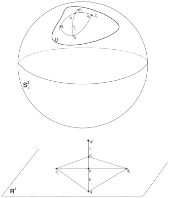
Figure 9.

Then since $0<\kappa$, Proposition 3.10.(3) applied to the quadruples $\{q,q_{1},q_{2},p\}$ and $\{q^{\prime},q^{\prime}_{1},q^{\prime}_{2},p^{\prime}\}$ implies that $h<pq$.
Now let $x\in\gamma_{2}$, $x$ between $p$ and $q$, and let $x^{\prime}\in\mathbb{R}^{2}$ s.t. $\triangle(q^{\prime}_{1}q^{\prime}_{2},x^{\prime})\cong\triangle(q_{1}q_{2},x)$ s.t. $x$ and $q^{\prime}$ are on different sides of the line $\stackrel{{\scriptstyle\longleftrightarrow}}{{q_{1}q_{2}}}$. Then, $x=p\;\Rightarrow\;xq>x^{\prime}q^{\prime}$, and $x=q\;\Rightarrow xq=0<x^{\prime}q^{\prime}=2h$, where, in this case $x^{\prime}=q^{\prime\prime}$. (See Figure 9.) Then it follows from a continuity argument that $\exists\,x_{0}\in\gamma_{2},\;x_{0}$ between $p$ and $q$, s.t. $x_{0}q=x_{0}^{\prime}q^{\prime}$, thus implying that $\{q_{1},q_{2},q,x\}\cong\{q^{\prime}_{1},q^{\prime}_{2},q^{\prime},x^{\prime}\}$. ∎

Remark 3.17.

$\{q_{1},q_{2},q,x\}$ is planar, while $\{q^{\prime}_{1},q^{\prime}_{2},q^{\prime},x^{\prime}\}$ is not planar.

3.2. The Wald Curvature vs. Gauss Curvature

The discussion above would be nothing more than a nice intellectual exercise where it not for the fact that the metric (Wald) and the classical (Gauss) curvatures coincide whenever the second notion makes sense, that is for smooth (i.e. of class $\geq\mathcal{C}^{2}$) surfaces in $\mathbb{R}^{3}$. More precisely the following theorem holds:

Theorem 3.18.

(Wald) Let $S\subset\mathbb{R}^{3},\;S\in\mathcal{C}^{m},\,m\geq 2$ be a smooth surface.
Then $\kappa_{W}(p)$ exists, for all $p\in S$, and $\kappa_{W}(p)=\kappa_{G}(p),\forall\,p\in M$.

Moreover, Wald also proved that a partial reciprocal theorem holds, more precisely he proved the following:

Theorem 3.19.

Let $M$ be a compact and convex metric space.
If $\kappa_{W}(p)$ exists, for all $p\in M$, then M is a smooth surface and $\kappa_{W}(p)=\kappa_{G}(p),\forall\,p\in\nolinebreak[4]M$.

Remark 3.20.

I one tries to restrict oneself, in the building of Definition 3.4. only to sd-quads, then Theorem 3.19. holds only if the following presumption is added:

Condition 3.21.

$M$ is locally homeomorphic to $\mathbb{R}^{2}$.

However the proof of this facts is involved and, as such, beyond the scope of this presentation. Therefore we shall restrict ourselves to a succinct description of the principal steps towards the proofs.
The basic idea is to show that if a metric $M$ space admits a Wald curvature at any point, than $M$ is locally homeomorphic to $\mathbb{R}^{2}$, thus any metric proprieties of $\mathbb{R}^{2}$ can be translated to $M$, (in particular the first fundamental form).
The first of these partial results is:

Theorem 3.22.

Let $M$ be a convex metric space. Then $M$ admits at most one Wald curvature $\kappa_{W}(p),\;\forall\,p\in M$.

Proof By Corollary 3.12. it suffices to prove that any disk neighborhood $B(p\,;\rho)\in\mathcal{N}(p)$ contains a non degenerate sd-quad.
Without loss of generality one can assume that $B(p\,;\rho)$ contains three points $p_{1},p_{2},p_{3}$ s.t. $d(p,p_{i})<\rho/2,\,i=1,2,3$. Then, by the convexity of $M$ it follows that $\exists\,q\in M$ s.t. $p\neq p_{2},p_{3}$ and $p_{2}q+p_{3}q=p_{2}p_{3}$. But $p_{2}p_{3}\leq pp_{2}+pp_{3}<\rho\Longrightarrow(pq<\rho/2)\vee(pp_{2}<\rho/2)$. In the first inequality holds, then $pq\leq pp_{2}+p_{2}q<\rho$, i.e $q\in B(p\,;\rho)$; and if the second one holds, then $pd\leq pp_{3}+p_{3}q<\rho$, i.e. $q\in B(p\,;\rho)$. But $p\neq q$, therefore $p,p_{2},p_{3},q$ are not linear.
$\Box$

Our next step will be to analyze those neighborhoods that display ”a normal behavior”, both metrically and curvature-wise: that is precisely those disk neighborhoods in which the Wald curvature is defined and ranges over a small, bounded set of values prescribed by the very radius of the disk:

Definition 3.23.

A disk neighborhood $B(p\,;\rho);\rho>0$ is called regular iff $\forall$ non-degenerate quadruple $Q\subset B(p\,;\rho)$ , $\kappa_{W}(Q)$ exists and $|\kappa_{W}(Q)|<\pi^{2}/16\rho^{2}$.

Remark 3.24.

If $\kappa_{W}(p)$ exists, then for any sufficiently small $\rho$, $B(p\,;\rho)$ will be regular.

It turns out that regular neighborhoods, in compact, convex spaces have the following ”nice” (i.e. Real Plane like) proprieties:

Proposition 3.25.

Let $M$ be a compact, convex metric space and let $B(p\,;\rho)\subset M$ be a regular neighborhood. Then if a non-degenerate quadruple $Q\subset B(p\,;\rho)$ contains two linear triples of points, then $Q$ is linear.

Proposition 3.26.

Let $M$ be a compact, convex metric space. Then:
$\forall\,p\in M$ and $\forall\,B(p\,;\rho)$ regular, $\exists\,q,r\in B(p\,;\rho)$ s.t. $p,q,r$ are not linear.

Proposition 3.27.

Any regular neighborhood $B(p\,;\rho)$ of a compact, convex metric space is strictly convex, i.e. $q,r\in B(p\,;\rho)\Longrightarrow int(qr)\subset B(p\,;\rho)$.

While the proof of this last Proposition is lengthy, that of the following important Corollary is not:

Corollary 3.28.

Let $B(p\,;\rho)$ be a regular neighborhood. Then, $\forall\,q,r\in B(p\,;\rho),\;\exists!\,qr$ and $int(qr)\subset B(p\,;\rho)$.

Proof.

By the convexity of $B(p\,;\rho)$ it follows the existence of at least one geodesic $qr,\;\forall\,q,r\in B(p\,;\rho)$. If $s\in int(q)r$, then by the proposition above we have that $s\in B(p\,;\rho)$. It follows that $B(p\,;\rho)$ contains all the geodesics with end points $q,r$. Hence, by Proposition 3.25. , the geodesic segment $qr$ is unique. ∎

We can now begin to prove that a compact, convex metric space locally mimics $\mathbb{R}^{2}$. We start by showing that the sinus function is defined on $M$, thus allowing for angle measure (hence for the definition of Polar Coordinates on regular neighbourhoods).
First, let $M$ be as before, and let $p\in M$ s.t. $\kappa_{W}{p}$ exists. Let $q,r\in B(p\,;\rho),q\neq p\neq r$, where $B(p\,;\rho)$ is a regular neighborhood of $p$. Then, $\forall\,x\in[0,min\{pq,pr\})$, define $q(x)\in pq,r(x)\in pr$ by: $d(p,q(x))=x=d(p,r(x))$, and let $d(x)=d(,q(x),r(x))$ (see Figure 10 bellow).

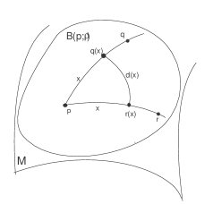
Figure 10.

Proposition 3.29.

The following limit exists:

$$\lim_{x\rightarrow 0}{\frac{d(x)}{x}}\,.$$

We omit the proof since it is rather involved (but canonical for any axiomatic approach to Euclidian Geometry – see, for instance, [B], [RR].)

Now we can define the measure of angles at $p$ :

Definition 3.30.

The measure of the angle $\angle(q,p,r))$ is given by:

$$m(\angle(q,p,r))\stackrel{{\scriptstyle\scriptstyle\triangle}}{{=}}2arcsin\Big{(}\frac{1}{2}\lim_{x\rightarrow 0}{\frac{d(x)}{x}}\Big{)}\,.$$

Remark 3.31.

The Definition above enables us to define Polar Coordinates on regular neighborhoods in the following manner:
Let $p_{1},p_{2}\in B(p\,;\rho)$ s.t. $p,p_{1},p_{2}$ are not collinear. (Such points exist by Proposition 3.26.). To every point $q\in B(p\,;\rho)$ we associate the following pair of real numbers (defining the Polar Coordinates of $q$ relative to the frame determined by $p,p_{1},p_{2}$): $(r(q),\theta(q))$, where

$$r(q)\stackrel{{\scriptstyle\scriptstyle\triangle}}{{=}}d(p,q)$$

and

$$\theta(q))\stackrel{{\scriptstyle\scriptstyle\triangle}}{{=}}\left\{\begin{array}[]{clclcr}\mbox{$m(\angle(q,p,p_{1}))$}&\mbox{if $|m(\angle(p_{2},p,p_{1}))-m(\angle(q,p,p_{1}))|=m(\angle(q,p,p_{1}))$ \,;}\\ \mbox{$2\pi-m(\angle(q,p,p_{1}))$}&\mbox{if $|m(\angle(p_{2},p,p_{1}))-m(\angle(q,p,p_{1}))|\neq m(\angle(q,p,p_{1}))$ \,.}\end{array}\right.$$

We can now safely state the foretold homomorphism result:

Proposition 3.32.

Any convex, compact metric space is locally homeomorphic to the real plane.

4. Computing Embedding Curvature

In this section we develop formulas for the computation of Embedding Curvature of Quadruples. First we follow the classical approach of Wald-Blumenthal that employs the so-called Cayley-Menger determinants (see bellow). Unfortunately, the formulas obtained, albeit precise are transcendental. Therefore we present, in the next subsection, the approximate formulas developed by C.V. Robinson.

4.1. Embedding Curvature – The Determinant Approach

Given a general metric quadruple $Q=Q(p_{1},p_{2},p_{3},p_{4})$, of distances
$d_{ij}=dist(p_{i},p_{j}),\;i=1,...,4$, we denote by $D(Q)=D(p_{1},p_{2},p_{3},p_{4})$ the following determinant:

(4.1) $$D(p_{1},p_{2},p_{3},p_{4})=\left|\begin{array}[]{ccccc}0&1&1&1&1\\ 1&0&d_{12}^{2}&d_{13}^{2}&d_{14}^{2}\\ 1&d_{12}^{2}&0&d_{23}^{2}&d_{24}^{2}\\ 1&d_{13}^{2}&d_{23}^{2}&0&d_{34}^{2}\\ 1&d_{14}^{2}&d_{24}^{2}&d_{34}^{2}&0\end{array}\right|$$

Then the embedding curvature $\kappa(Q)$ of $Q$ is given – depending upon the embedding space (i.e. upon the sign of the curvature) – by the following formulae:

(4.2) $$\kappa(Q)=\left\{\begin{array}[]{clclcrcr}\mbox{0}&\mbox{if $D(Q)=0$\,;}\\ \mbox{$\kappa,\,\kappa<0$}&\mbox{if $det({\cosh{\sqrt{-\kappa}\cdot d_{ij}}})=0$\,;}\\ \mbox{$\kappa,\,\kappa>0$}&\mbox{if $det(\cos{\sqrt{\kappa}\cdot d_{ij}})$ and $\sqrt{\kappa}\cdot d_{ij}\leq\pi$}\\ &\mbox{\;\; and all the principal minors of order $3$ are $\geq 0$.}\end{array}\right.$$

The determinant $D(Q)=D(p_{1},p_{2},p_{3},p_{4})$ is called the Cayley-Menger determinant (of the points $p_{1},...p_{4}$) and, in order to prove (4.2) we need first to investigate some of its properties.
We start with the following

Lemma 4.1.

Let: $p_{1},...,p_{4}$ be points in $\mathbb{R}^{3}$. Then:

(4.3) $$Gram(\overrightarrow{p_{1}p_{2}},\overrightarrow{p_{1}p_{3}},\overrightarrow{p_{1}p_{4}})=\frac{1}{8}D(p_{1},p_{2},p_{3},p_{4})\,;$$

where

$$Gram(\overrightarrow{p_{1}p_{2}},\overrightarrow{p_{1}p_{3}},\overrightarrow{p_{1}p_{4}})\stackrel{{\scriptstyle def}}{{=}}det(\overrightarrow{p_{1}p_{i}}\cdot\overrightarrow{p_{1}p_{j}})_{i,j=2,3,4}$$

(Here ”$\cdot$” denotes the standard scalar (dot) product in $\mathbb{R}^{3}$.)

Proof.

Use expansion and manipulation of determinants. ∎

Since is a known fact that:

$$Gram(\overrightarrow{p_{1}p_{2}},\overrightarrow{p_{1}p_{3}},\overrightarrow{p_{1}p_{4}})=\big{(}Vol(p_{1},p_{2},p_{3},p_{4})\big{)}^{2}\,;$$

where $Vol(p_{1},p_{2},p_{3},p_{4})$ denotes the (un-oriented) volume of the parallelepiped determined by the vertices $p_{1},...,p_{4}$ (and with edges $\overrightarrow{p_{1}p_{2}},\overrightarrow{p_{1}p_{3}},\overrightarrow{p_{1}p_{4}}$); formula (2.3) shows that:

(4.4) $$D(p_{1},p_{2},p_{3},p_{4})=8\big{(}Vol(p_{1},p_{2},p_{3},p_{4})\big{)}^{2}\,.$$

Therefore the following assertion is immediate:

Proposition 4.2.

The points $p_{1},...,p_{4}$ are the vertices of a simplex in $\mathbb{R}^{3}$ iff $D(p_{1},p_{2},p_{3},p_{4})\neq 0$.̇

However, we can prove the much strong result bellow:

Theorem 4.3.

Let $d_{ij}>0\,,1\leq 4\,,i\neq j$.
Then there exists a simplex $T=T(p_{1},...,p_{4})\subseteq\mathbb{R}^{3}$ s.t. $dist(x_{i},x_{j})=d_{ij}\,,i\neq j$; iff $D(p_{i},p_{j})<0\,,(\forall)\,\{i,j\}\subset\{1,...,4\}$ and
$D(p_{i},p_{j},p_{k})>0\,,(\forall)\,\{i,j,k\}\subset\{1,...,4\}$;
where, for instance,

$$D(p_{1},p_{2})=\left|\begin{array}[]{ccc}0&1&1\\ 1&0&d_{12}^{2}\\ 1&d_{12}^{2}&0\end{array}\right|\,$$

and

$$D(p_{1},p_{2},p_{3})=\left|\begin{array}[]{cccc}0&1&1&1\\ 1&0&d_{12}^{2}&d_{13}^{2}\\ 1&d_{12}^{2}&0&d_{23}^{2}\\ 1&d_{13}^{2}&d_{23}^{2}&0\end{array}\right|\,;$$

etc…

In fact, the necessary and sufficient condition above can be relaxed, indeed one can also show that the following holds:

Proposition 4.4.

Let $d_{ij}>0\,,1\leq 4\,,i\neq j$.
Then there exists a simplex $T=T(p_{1},...,p_{4})\subseteq\mathbb{R}^{3}$ s.t. $dist(x_{i},x_{j})=d_{ij}\,,i\neq j$; iff $D(p_{1},p_{2},p_{3},p_{4})\neq 0$ and $sign\,D(p_{1},p_{2},p_{3},p_{4})=+1$ .

Proof.

(Sketch) Sufficient to show (by using standard operations on determinants) that:

$$D(p_{1},p_{2},p_{3})D(p_{1},...,\hat{p_{i}},...,p_{4})=M_{i4}^{2}+D(p_{1},...,\hat{p_{i}},...,p_{4})D(p_{1},p_{2},p_{3},p_{4})\,;$$

where $M_{i4}$ is the cofactor (in $D$) of $d_{i4}^{2}$, and were we used the notation:
$\{p_{1},...,\hat{p_{i}},...,p_{4}\}=\{p_{1},p_{2},p_{3},p_{4}\}\setminus\{p_{i}\}$. ∎

Proving the formula for the spherical and hyperbolical cases would prove to be to technical for this limited exposition; suffice to say that they essentially reproduce the proof given in the Euclidian case, and tacking into account the fact that performing computations in the spherical (resp. hyperbolic) metric one has to replace the distances $d_{ij}$ by $\cos{d_{ij}}$ (resp. $\cosh{d_{ij}}$).

4.2. Embedding Curvature – Approximate Formulas

The formulas we just developed in are not only transcendental, but also the computed curvature may fail to be unique (see preceding section). However, uniqueness is guaranteed for sd-quads. Moreover, the relatively simple geometric setting of sd-quads allows for the development of simple (i.e. rational) formulas for the approximation of the Embedding Curvature.

Proposition 4.5.

Given the metric quadruple $Q=Q(p_{1},p_{2},p_{3},p_{4})$, of distances
$d_{ij}=dist(p_{i},p_{j}),\;i=1,...,4$, the embedding curvature $\kappa(Q)$ is well approximated by:

(4.5) $$K(Q)=\frac{6(\cos{\angle_{0}2}+\cos{\angle_{0}2^{\prime}})}{d_{24}(d_{12}\sin^{2}({\angle_{0}2})+d_{23}\sin^{2}({\angle_{0}2^{\prime}}))}$$

where: $\angle_{0}2=\angle(p_{1}p_{2}p_{4})\,,\;\angle_{0}2^{\prime}=\angle(p_{3}p_{2}p_{4})$ represent the angles of the Euclidian triangles of sides $d_{12},d_{14},d_{24}$ and $d_{23},d_{24},d_{34}$ , respectively.
The error $R$ can be estimated by using the following inequality:

(4.6) $$|R|=|R(Q)|=|\kappa(Q)-K(Q)|<4\kappa^{2}(Q)diam^{2}(Q)/\lambda(Q)$$

where we put: $\lambda(Q)=d_{24}(d_{12}\sin{\angle_{0}2}+d_{23}\sin{\angle_{0}2^{\prime}})/S^{2}$, and where $S=Max\{p,p^{\prime}\};\;\\ 2p=d_{12}+d_{14}+d_{24}\,,\;2p^{\prime}=d_{32}+d_{34}+d_{24}$.

Proof The basic idea of the proof is to recreate, in a general metric setting, the Gauss Map – in this case one measures the curvature by the amount of ”bending” one has to apply to a general planar quadruple so that it may be ”straightened” (i.e. isometrically embedded as a sd-quad) in some $S_{\kappa}$.
Consider two plane triangles $\triangle p_{1}p_{2}p_{4}$ and $\triangle p_{2}p_{3}p_{4}$, and denote by $\triangle p_{1,k}p_{2,k}p_{4,k}$ and $\triangle p_{2,k}p_{3,k}p_{4,k}$ their respective isometric embeddings into $\mathcal{S}_{k}$. Then $p_{i,k}p_{j,k}$ will denote the geodesic (of $\mathcal{S}_{k}$) through $p_{i,k}$ and $p_{j,k}$. Also, let $\angle_{k}2$ and $\angle_{k}2^{\prime}$ denote, respectively, the following angles of $\triangle p_{1,k}p_{2,k}p_{4,k}$ and $\triangle p_{2,k}p_{3,k}p_{4,k}$ : $\angle_{k}2=\angle p_{1,k}p_{2,k}p_{4,k}$ and $\angle_{k}2^{\prime}=\angle p_{2,k}p_{3,k}p_{4,k}$. (See Fig. 11)

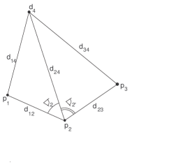
Figure 11.

But $\angle_{k}2$ and $\angle_{k}2^{\prime}$ are strictly increasing as functions of $k$. Therefore the equation

(4.7) $$\angle_{k}2+\angle_{k}2^{\prime}=\pi$$

has at most one solution $k^{*}$, i.e. $k^{*}$ represents the unique value for which the points $p_{1},p_{2},p_{4}$ are on a geodesic in $\mathcal{S}_{k}$ (for instance on $p_{1}p_{4}$).
But that means that $k^{*}$ is precisely the Embedding Curvature, i.e. $k^{*}=\kappa(Q)$ , where $Q=Q(p_{1},p_{2},p_{3},p_{4})$.
Equation $(4.7)$ is equivalent to

$$\cos^{2}\frac{\angle_{k^{*}}2}{2}\;+\;\cos^{2}\frac{\angle_{k^{*}}2^{\prime}}{2}\,=\,1$$

The basic idea being the comparison between metric triangles with equal sides, embedded in $\mathcal{S}_{0}$ and $\mathcal{S}_{k}$, respectively, it is natural to consider instead of the previous equation, the following:

(4.8) $$\theta(k,2)\cdot\cos^{2}\frac{\angle_{0}2}{2}\;+\;\theta(k,2^{\prime})\cdot\cos^{2}\frac{\angle_{0}2^{\prime}}{2}\,=\,1$$

where we denote:

$$\theta(k,2):=\frac{\cos^{2}\frac{\angle_{k^{*}}2}{2}}{\cos^{2}\frac{\angle_{0}2}{2}}\,;\;\;\theta(k,2^{\prime}):=\frac{\cos^{2}\frac{\angle_{k^{*}}2^{\prime}}{2}}{\cos^{2}\frac{\angle_{0}2}{2}}\,.$$

Since we want to approximate $\kappa(Q)$ by $K(Q)$ we shall resort – naturally – to expansion into MacLaurin series. We are able to do this because of the existence of the following classical formulas:

$$\cos^{2}\frac{\angle_{k}2}{2}=\frac{\sin({p\sqrt{k}})\cdot\sin({d\sqrt{k}})}{\sin({d_{12}\sqrt{k}})\cdot\sin({d_{24}\sqrt{k})}}\,;\;k>0\,;$$

$$\cos^{2}\frac{\angle_{k}2}{2}=\frac{\sinh({p\sqrt{k}})\cdot\sinh({d\sqrt{k}})}{\sinh({d_{12}\sqrt{k})}\cdot\sinh({d_{24}\sqrt{k}})}\,;\;k<0\,;$$

and, of course

$$\cos^{2}\frac{\angle_{0}2}{2}=\frac{pd}{d_{12}d_{24}}\,;$$

were: $d=p-d_{14}=(d_{12}+d_{24}-d_{14})/2\,.$
By using the development into series of $f_{1}(x)=\frac{\sin{\sqrt{x}}}{{\sqrt{x}}}$ and $f_{2}(x)=\frac{\sinh{\sqrt{x}}}{{\sqrt{x}}}$; one (easily) gets the desired expansion for $\theta(k,2)$:

(4.9) $$\theta(k,2)=1+\frac{1}{6}kd_{12}d_{24}\big{(}\cos(\angle_{0}{2})-1\big{)}+r\,;$$

where: $|r|<\frac{3}{8}k^{2}p^{4}$ , for $|kp^{2}|<1/16$ . By applying (4.9.) to (4.8), we receive:

(4.10) $$[1+\frac{1}{6}k^{*}d_{12}d_{24}\big{(}\cos(\angle_{0}{2})-1\big{)}+r]\cos^{2}\frac{\angle_{0}2}{2}\;+\;$$

$$[1+\frac{1}{6}k^{*}d_{23}d_{24}\big{(}\cos(\angle_{0}{2^{\prime}})-1\big{)}+r^{\prime}]\cos^{2}\frac{\angle_{0}2^{\prime}}{2}=1\,;$$

for: $|r|+|r^{\prime}|<\frac{3}{4}(k^{*})^{2}(Max\{p,p^{\prime}\})^{4}=\frac{3}{4}(k^{*})^{2}S^{4}$ .
By solving linear equation (in variable $k^{*}$) (4.10) and using some elementary trigonometric transformation one has:

$$k^{*}=\frac{6(\cos{\angle_{0}{2}}+\cos{\angle_{0}{2^{\prime}}})}{d_{24}(d_{12}\sin^{2}({\angle_{0}{2}})+d_{23}\sin^{2}({\angle_{0}{2^{\prime}}}))}+R$$

where:

$$|R|<\frac{12(|r|+|r^{\prime}|)}{d_{24}\big{(}d_{12}\sin^{2}({\angle_{0}{2}})+d_{23}\sin^{2}({\angle_{0}2^{\prime}})\big{)}}<\frac{9(k^{*})^{2}\max\{p,p^{\prime}\}}{d_{24}\big{(}d_{12}\sin^{2}({\angle_{0}{2}})+d_{23}\sin^{2}({\angle_{0}2^{\prime}})\big{)}}$$

But $k^{*}\equiv\kappa(Q)$ so we get the desired formula (4.5) .
To prove the correctness of the bound (4.6) one has only to observe that:

$$S=Max\{p,p^{\prime}\}<2diam(Q),\;\big{(}diam(Q)=\max_{1\leq i<j\leq 4}\{d_{ij}\}\big{)},$$

and perform the necessary arithmetic manipulations.
$\Box$

Remark 4.6.

(a) The function $\lambda=\lambda(Q)$ is continuous and 0-homogenous as a function of the $d_{ij}$-s. Moreover: $\lambda(Q)\geq 0$ and $\lambda(Q)=0\Leftrightarrow\sin{\angle_{0}2}=\sin{\angle_{0}2^{\prime}}=0$, i.e. iff $Q$ is linear. [Therefore for sd-quads $\lambda(Q)>0$ and, moreover, $\lambda(Q)\rightarrow 0\Rightarrow\\ Q\rightarrow linearity$.]
                  (b) Since $\lambda(Q)\neq 0$ it follows that: $K(Q)\in\mathbb{R}$ for any quadrangle $Q$.
In addition: $sign(k(Q))=sign(K(Q))$.
                  (c) If $Q$ is any sd-quad, then $\kappa^{2}(Q)diam^{2}(Q)/\lambda(Q)<\infty$. Moreover, if $\lambda(Q)\gg{/}\;\>0$, then $\kappa^{2}(Q)diam^{2}(Q)/\lambda(Q)\gg{/}\;\>0\,$ i.e. $|R|$ is small if $Q$ is not close to linearity.
In this case $|R(Q)|\sim diam^{2}(Q)$ (for any given $Q$).

Since the Gaussian curvature $k_{G}(p)$ at a point $p$ is given by:

$$k_{G}(p)=\lim_{n\rightarrow 0}{\kappa(Q_{n})}\,;$$

where $Q_{n}\rightarrow Q=\Box p_{1}pp_{3}p_{4}\,;\;diam(Q_{n})\rightarrow 0$,from Remark 4.6.(c) we immediately infer that the following holds:

Theorem 4.7.

Let $S$ be a differentiable surface. Then, for any point $p\in S$:

$$k_{G}(p)=\lim_{n\rightarrow 0}{K(Q_{n})}\,;$$

for any sequence $\{Q_{n}\}$ of sd-quads that satisfy the following condition:

$$Q_{n}\rightarrow Q=\Box p_{1}pp_{3}p_{4}\,;\;diam(Q_{n})\rightarrow 0\,.$$

Remark 4.8.

In the following special cases even ”nicer” formulas are obtained:

1. If $d_{12}=d_{32}$, then

   (4.11) $$K(Q)=\frac{12}{d_{13}\cdot d_{24}}\cdot\frac{\cos{\angle_{0}2}+\cos{\angle_{0}2^{\prime}}}{\sin^{2}{\angle_{0}2}+\sin^{2}{\angle_{0}2^{\prime}}}\,;$$

   (here we have of course: $d_{13}=2d_{12}=2d_{32}$); or, expressed as a function of distances alone:

   (4.12) $$K(Q)=12\frac{2d_{12}^{2}+2d_{24}^{2}-d_{14}^{2}-d_{13}^{2}}{8d_{12}^{2}d_{24}^{2}-(d_{12}^{2}+d_{24}^{2}-d_{14}^{2})^{2}-(d_{12}^{2}+d_{24}^{2}-d_{34}^{2})^{2}}$$

2. If $d_{12}=d_{32}=d_{24}$ and if the following condition also holds:

3. $\angle_{0}2^{\prime}=\pi/2$; i.e. if $d_{34}^{2}=d_{12}^{2}+d_{24}^{2}$ or, considering (2), also: $d_{34}^{2}=2d_{12}^{2}$
   then

   (4.13) $$K(Q)=\frac{6\cos{\angle_{0}2}}{d_{12}(1+\sin^{2}{\angle_{0}2})}=\frac{2d_{12}^{2}-d_{14}^{2}}{4d_{12}^{4}+4d_{14}^{2}d_{12}^{2}-d_{14}^{4}}\,.$$

5. Appeendix 1 – The Menger and Haantjes Curvatures

Better known than the Wald Curvature, the Menger Curvature is a metric definition of curvature of curves, as is the Haantjes Curvature. As such they can be employed as sectional curvatures to approximate curvature of triangulated surfaces.
We begin by introducing the the Menger Curvature: this is a metric expression for the circum-radius of a triangle, based upon elementary high-school formulas:

Definition 5.1.

Let $(M,d)$ be a metric space, and let $p,q,r\in M$ be three distinct points. Then:

$$K_{M}(p,q,r)=\frac{\sqrt{(pq+qr+rp)(pq+qr-rp)(pq-qr+rp)(-pq+qr+rp)}}{pq\cdot qr\cdot rp}\,;$$

is called the Menger Curvature of the points $p,q,r$.

We can now define the Menger Curvature at a given point by passing to the limit:

Definition 5.2.

Let (M,d) be a metric space and let $p\in M$ be an accumulation point. Then $M$ has at $p$ Menger Curvature $\kappa_{M}(p)$ iff
$\forall\,\varepsilon>0,\;\exists\,\delta>0$ s.t. $d(p,p_{i})<\delta\,;\;i=1,2,3\;\Longrightarrow|K(Q)-\kappa_{M}(p)|<\varepsilon$.

Remark 5.3.

The apparent equivalent notion of Alt Curvature, in which one uses only two points converging to the third, is in fact more general, where we define the Arp curvature by:

Definition 5.4.

Let (M,d) be a metric space and let $P\in M$ be an accumulation point. Then $M$ has at $p$ Alt Curvature $\kappa_{A}(p)$ iff the following limit exists

$$\kappa_{A}(p)\stackrel{{\scriptstyle\scriptstyle\triangle}}{{=}}\lim_{q,r\rightarrow p}K(p,q,r)\,.$$

However, both $\kappa_{M}(p)$ and $\kappa_{A}(p)$ suffer from the same imperfection: since they are both modelled closely after the Euclidian Plane, they convey this Euclidian type of curvature upon the space they are defined on. However, the next definition doesn’t mimic closely $\mathbb{R}^{2}$ so it better fitted for generalizations:

Definition 5.5.

Let (M,d) be a metric space and let $c:I=[0,1]\stackrel{{\scriptstyle\sim}}{{\rightarrow}}M$ be a homeomorphism, and let $p,q,r\in c(I),\;q,r\neq p$. Denote by $\widehat{qr}$ the arc of $c(I)$ between $q$ and $r$, and by $qr$ segment from $q$ to $r$. (See Figure 12 bellow.)

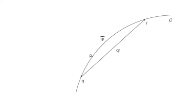
Figure 12.

Then $c$ has Haantjes Curvature $\kappa_{H}(p)$ at the point $p$ iff:

$$\kappa_{H}^{2}(p)=24\lim_{q,r\rightarrow p}\frac{l(\widehat{qr})-d(q,r)}{\big{(}l(\widehat{qr})\big{)}^{3}}\,\,;$$

where ”$l(\widehat{qr})$” denotes the length of $\widehat{qr}$.

Remark 5.6.

$\kappa_{H}$ exists only for rectifiable curves, but if $\kappa_{M}$ exists at any point $p$ of $c$, then $c$ is rectifiable.

Remark 5.7.

Evidently we have the following relationship between curvatures:

$$\exists\,\kappa_{M}\;\Longrightarrow\;\exists\,\kappa_{A}\,.$$

while

$$\exists\,\kappa_{A}\;\Longrightarrow/\;\;\;\exists\,\kappa_{M}\,.$$

However, we can prove the following theorem:

Theorem 5.8.

Let $c:I\rightarrow M$ be a rectifiable curve, and let $p\in M$.
If $\kappa_{A}$ (or $\kappa_{M}$) exists, then $\kappa_{H}(p)$ exists and

$$\kappa_{A}=\kappa_{H}(p)\,.$$

Remark 5.9.

This last result and the Remark preceding it allow as to employ any of the curvatures above in estimating curvatures of smooth curves on triangulated surfaces.

6. Appendix 2 – The Rinow Curvature

The curvatures introduced before may seem a bit archaic in comparison to the more fashionable approach of comparison triangles, with their ar reaching applications. We present here one of these comparison criteria and show its equivalence with the Wald curvature. We start with the following definition:

Definition 6.1.

Let $(M,d)$ be a metric space, together with the intrinsic metric induced by $d$. Let $R=int(R)\subseteq M$ be a region of $M$. We say that $R$ is a region of curvature $\leq\kappa$ ($\kappa\in\mathrm{R}$) iff

1. $\forall p,q\in R\;,\exists$ a geodesic segment $pq\subset R$;

2. $\forall\,T(p,q,r)\subset R$ is isometrically embeddable in $\mathcal{S}_{\kappa}$;

3. If $T(p,q,r)\subset R$ and $x\in pq,y\in pr$, and if the points $p_{\kappa},q_{\kappa},r_{\kappa},x_{\kappa},y_{\kappa}\in\mathcal{S}_{\kappa}$ satisfy the following conditions:

   1. $T(p,q,r)\cong T(p_{\kappa},q_{\kappa},r_{\kappa})$;

   2. $T(p,q,x)\cong T(p_{\kappa},q_{\kappa},x_{\kappa})$;

   3. $T(p,r,y)\cong T(p_{\kappa},r_{\kappa},y_{\kappa})$;

   then $xy\leq x_{\kappa}y_{\kappa}$.

By replacing the condition: ”$xy\leq x_{\kappa}y_{\kappa}$” with: ”$xy\geq x_{\kappa}y_{\kappa}$”, we obtain the definition of a region of curvature $\geq\kappa$. (See Fig. 13.)

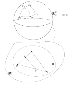
Figure 13.

We now pass to the localization of the Definition above:

Definition 6.2.

Let $(M,d)$ be a metric space, together with the intrinsic metric induced by $d$, and let $p\in M$ be an accumulation point. Then $M$ has at $p$ Rinow Curvature $\kappa_{R}(p)$ iff
(i) $\exists/\,\,N\in\mathcal{N}(p),\,N$ linear;
(ii) $\forall\,\varepsilon>0,\;\exists\,\delta.0$, s.t.$B(p;\delta)$ is (a) a region of Rinow curvature $\leq\kappa_{R}(p)+\varepsilon$ and (b) a region of Rinow curvature $\geq\kappa_{R}(p)-\varepsilon$.

While its greater generality endows the Rinow curvature with more flexibility in applications and makes it easier in generalization, it is even more difficult to compute than Wald Curvature. However this quandary was has an almost ideal solution, due to Kirk (see [K]), solution which we briefly expose here:

Definition 6.3.

Let $M$ be a compact, convex metric space, and let $p\in M$.
If $\kappa_{W}(p)$ exists, then $\kappa_{R}(p)$ exists, and $\kappa_{R}(p)=\kappa_{W}(p)$.

Unfortunately, since $\kappa_{R}(p)$ makes no presumption of dimensionality, the existence of $\kappa_{R}(p)$ does not imply the existence of $\kappa_{W}(p)$.

Counterexample 6.4.

Let $M\equiv\mathbb{R}^{3}$. Then $\kappa_{R}(p)\equiv 0$ but $\kappa_{W}(p)$ does not exist at any point, since every neighborhood contains linear quadruples.

The solution (due to Kirk) of this problem is to consider the Modified Wald curvature $\kappa_{WK}$, defined as follows:

Definition 6.5.

Let $(M,d)$ be a metric space, together with the intrinsic metric induced by $d$, and let $p\in M$. Then $M$ has at $p$ Modified Wald curvature Curvature $\kappa_{WK}(p)$ iff
(i) $\exists/\,\,N\in\mathcal{N}(p),\,N$ linear;
(ii) $\forall\,\varepsilon>0,\;\exists\,\delta.0$, s.t. if $Q\subset B(p;\delta)$ is a non-degenerate sd-quad, then $\kappa_{W}(Q)$ exists and $|\kappa_{WK}(p)-\kappa_{W}(Q)|<\varepsilon$.

Remark 6.6.

$\exists\,\kappa_{W}(p)\;\Longrightarrow\;\exists\,\kappa_{WK}(p)$ but $\exists\kappa_{KW}(p)\Longrightarrow/\;\;\;\kappa_{W}(p)$.

This modified curvature indeed represents the wished for solution, as proved by the following to Theorems:

Theorem 6.7.

Let $(M,d)$ be a metric space. Then:
                  $\exists\,\kappa_{R}(p)\;\Longrightarrow\;\exists\,\kappa_{WK}(p)$ and $\kappa_{R}(p)=\kappa_{WK}(p)$.

Theorem 6.8.

Let $(M,d)$ be a metric space together with the associated intrinsic metric, and let $p\in M$. Then, if
(i) $\kappa_{WK}(p)$;
and if
(ii) $\exists\,B(p;\rho)\in\mathcal{N}(p)$, s.t. $qr\subset B(p;\rho),\;\forall q,r\in B(p;\rho)$;
then $\kappa_{R}(p)$ exists and $\kappa_{R}(p)=\kappa_{WK}(p)$.

7. Appendix 3 – The Radius Formula

The Cayley-Menger determinant allows one to express not only the volume and area of simplices in $\mathbb{R}^{n}$ but (as expected) it may be used to compute the radius of the circumscribed sphere around an Euclidian simplex. To be more precise, we have the following result:

Theorem 7.1.

1. The radius $R=R(p_{1},p_{2},p_{3},p_{4})$ of the sphere circumscribed around the tetrahedron $T(p_{1},p_{2},p_{3},p_{4})\in\mathbb{R}^{3}$ is given by:

   $$R^{2}=-\frac{1}{2}\frac{\Delta(p_{1},p_{2},p_{3},p_{4})}{D(p_{1},p_{2},p_{3},p_{4})}$$

   where:

   $$\Delta(p_{1},p_{2},p_{3},p_{4})=\left|\begin{array}[]{cccc}0&d_{12}^{2}&d_{13}^{2}&d_{14}^{2}\\ d_{12}^{2}&0&d_{23}^{2}&d_{24}^{2}\\ d_{13}^{2}&d_{23}^{2}&0&d_{34}^{2}\\ d_{14}^{2}&d_{24}^{2}&d_{34}^{2}&0\end{array}\right|$$

2. The points $p_{1},p_{2},p_{3},p_{4},p_{5}\in\mathbb{R}^{3}$ are coplanar or co-spherical iff

   $$\Delta(p_{1},p_{2},p_{3},p_{4},p_{5})=0\;.$$

Proof

1. If $p_{0}\in\mathbb{R}^{3}$ is s.t. $d_{0i}=R,\;i=1,...,5$, then by direct computation we obtain:

   $$\Gamma(p_{0},...,p_{5})=-2R^{2}\Gamma(p_{1},...,p_{5})-\Delta(p_{1},p_{2},p_{3},p_{4},p_{5})\,;$$

   from which the desired formula follows immediately if we chose $p_{0}$ as the center of the sphere circumscribed around the points $p_{1},p_{2},p_{3},p_{4},p_{5}$.

$(\Longrightarrow)$ Let $\{x^{1},x^{2},x^{3}\}$ be any orthonormal coordinate frame for $\mathbb{R}^{3}$, and let $p_{i}^{j};\;i=1,...,5;j=1,2,3$; represent the coordinates of the points $p_{1},p_{2},p_{3},p_{4},p_{5}$ relative to this coordinate system. Then $p_{1},p_{2},p_{3},p_{4},p_{5}$ belong to the same sphere or plane iff $\exists\;(a,b,c_{j})\neq(0,0,0),\;j=1,2,3$; s.t.

$$a||p_{i}||^{2}+b+\sum_{j=1}^{3}c_{j}p_{i}^{j}\,;\;i=1,...,5.$$

Then $\Delta_{1}=\Delta_{2}=0$, where:

$$\Delta_{1}(p_{1},p_{2},p_{3},p_{4},p_{5})=\left|\begin{array}[]{ccccc}||p_{1}||^{2}&1&p_{1}^{1}&p_{1}^{2}&p_{1}^{3}\\ ||p_{2}||^{2}&1&p_{2}^{1}&p_{2}^{2}&p_{2}^{3}\\ ||p_{3}||^{2}&1&p_{3}^{1}&p_{3}^{2}&p_{3}^{3}\\ ||p_{4}||^{2}&1&p_{4}^{1}&p_{4}^{2}&p_{4}^{3}\\ ||p_{5}||^{2}&1&p_{5}^{1}&p_{5}^{2}&p_{5}^{3}\end{array}\right|$$

and

$$\Delta_{2}(p_{1},p_{2},p_{3},p_{4},p_{5})=\left|\begin{array}[]{ccccc}1&||p_{1}||^{2}&-2p_{1}^{1}&-2p_{1}^{2}&-2p_{1}^{3}\\ 1&||p_{2}||^{2}&-2p_{2}^{1}&-2p_{2}^{2}&-2p_{2}^{3}\\ 1&||p_{2}||^{2}&-2p_{3}^{1}&-2p_{3}^{2}&-2p_{3}^{3}\\ 1&||p_{2}||^{2}&-2p_{4}^{1}&-2p_{4}^{2}&-2p_{4}^{3}\\ 1&||p_{2}||^{2}&-2p_{5}^{1}&-2p_{5}^{2}&-2p_{5}^{3}\end{array}\right|$$

Therefore $\Delta_{1}\cdot\Delta_{2}^{t}=0$. But $\Delta_{1}\cdot\Delta_{2}^{t}=\Delta(p_{1},p_{2},p_{3},p_{4},p_{5})$, so this implication is proven.
   $(\Longleftarrow)$ $\Delta(p_{1},p_{2},p_{3},p_{4},p_{5})=0\;\Longrightarrow\;\Delta_{1}=0$ and there exist numbers $(a,b,c_{j})\neq(0,0,0),\;j=1,2,3$; s.t.

$$a||p_{i}||^{2}+b+\sum_{j=1}^{3}c_{j}p_{i}^{j}=0\,;\;i=1,...,5;$$

i.e. $p_{1},p_{2},p_{3},p_{4},p_{5}$ belong to the plane or the sphere given by the equation

$$a||X||^{2}+b+c\sum_{j=1}^{3}c_{j}X=0\,;\;X=(x_{1},x_{2},x_{3})\,.$$

$\Box$

References

- [Ba1] Banchoff, T.A. – Critical points and curvature for embedded polyhedra, J. Differential Geometry, 1 (1967), 257-268.
- [Ba2] Banchoff, T.A. – Critical Points and Curvature for Embedded Polyhedral Surfaces, Amer. Math. Monthly, 77 (1970), 475-485.
- [Be] Berger, M. – Geometry I, Universitext, Spinger-Verlag, 1987.
- [B] Blumenthal, L. M. Distance Geometry – Theory and Applications, Claredon, 1953.
- [BM] Blumenthal, L. M. and Menger, K. – Studies in Geometry, Freeman and Co., 1970.
- [BH] Bridson, M. R. and Haefliger, A. – Metric spaces of non-positive curvature , Grundlehren der mathematischen Wissenschaften, Springer-Verlag, Berlin, 1999.
- [BBI] Burago, D. , Burago, Y. and Ivanov, S. – A Course in Metric Geometry, GSM, AMS, RI, 2000.
- [BCM] Borrelli, V. Cazals, F. and Morvan, J.-M. – On the angular defect of triangulations and the poitwise approximation of Curvatures, Computer Aided Geometric Designs, 20, pp. 319-341, 2003.
- [CMS] Cheeger, J. , Müller, W. , and Schrader, R. – On the Curvature of Piecewise Flat Spaces, Comm. Math. Phys. , 92, 1984, 405-454.
- [C-SM] Cohen-Steiner, D. and Morvan, J.-M. – Restricted Delaunay triangulations and normal cycle, preprint, 2003.
- [F] Fu, J. H. G. – Convergence of Curvatures in Secant Approximation, J. Differential Geometry, 37, 1993, 177-190.
- [G+] Mikhail Gromov – Metric structures for Riemannian and non-Riemannian spaces, Progress in Mathematics 152, Birkhauser, Boston, 1999.
- [K] Kirk, W. A. – On Curvature of a Metric Space at a Point, Pacific J. Math. 14: 195-198, 1964.
- [LWZL] Liu, G.H. , Wong, Y.S. , Zhang, Y.F. and Loh, H.T. – Adaptive fairing of digitized point data with discrete curvature, Comuter Aided Design, vol. 34(4), 309-320, 2002.
- [MD] Maltret, J.-L. and Daniel, M. – Discrete curvatures and applications: a survey, preprint, 2003.
- [P] Pajot, H. – Analytic Capacity, Rectificabilility, Menger Curvature and the Cauchy Integral, LNM 1799, Springer, Berlin, 2002.
- [RR] Ramsay, A. and Richtmayer, R.D. – Introduction to Hyperbolic Geometry, Universitext, Spinger-Verlag, 1991.
- [Rat] Ratcliffe, J.C. : Foundations of Hyperbolic Manifolds, GTM 194, Springer Verlag, N.Y., 1994.
- [R] Robinson, C.V. – A Simple Way of Computing the Gauss Curvature of a Surface, Reports of a Mathematical Colloquium, Second Series, Issue 5-6, 16-24, 1944.
- [SMSER] Surazhsky, T. , Magid, E. , Soldea, O. , Elber, G. and Rivlin, E. – A Comparison of Gaussian and Mean Curvatures Estimation Methods on TRiangular Meshes, preprint, 2003.
- [T] Troyanov, M. – Tangent Spaces to Metric Spaces: Overview and Motivations, preprint, 2003.