On an explicit finite difference method for fractional diffusion equations

Abstract

A numerical method to solve the fractional diffusion equation, which could also be easily extended to many other fractional dynamics equations, is considered. These fractional equations have been proposed in order to describe anomalous transport characterized by non-Markovian kinetics and the breakdown of Fick’s law. In this paper we combine the forward time centered space (FTCS) method, well known for the numerical integration of ordinary diffusion equations, with the Grünwald-Letnikov definition of the fractional derivative operator to obtain an explicit fractional FTCS scheme for solving the fractional diffusion equation. The resulting method is amenable to a stability analysis à la von Neumann. We show that the analytical stability bounds are in excellent agreement with numerical tests. Comparison between exact analytical solutions and numerical predictions are made.

url]http://www.unex.es/fisteor/santos/sby.html

1 Introduction

Fractional differential equations have been a highly specialized and isolated field of mathematics for many years [1]. However, in the last decade there has been increasing interest in the description of physical and chemical processes by means of equations involving fractional derivatives and integrals. This mathematical technique has a broad potential range of applications [2]: relaxation in polymer systems, dynamics of protein molecules and the diffusion of contaminants in complex geological formations [3, 4, 5] are some of the most recently suggested [6].

Fractional kinetic equations have proved particularly useful in the context of anomalous slow diffusion (subdiffusion) [7]. Anomalous diffusion is characterized by an asymptotic behavior of the mean square displacement of the form

$$\left<x^{2}(t)\right>\sim\frac{2K_{\gamma}}{\Gamma(1+\gamma)}t^{\gamma}\;,$$ (1)

where $\gamma$ is the anomalous diffusion exponent. The process is usually referred to as subdiffusive when $0<\gamma<1$. Ordinary (or Brownian) diffusion corresponds to $\gamma=1$ with $K_{1}=D$ (the diffusion coefficient). From a continuous (macroscopic) point of view, the diffusion process is described by the diffusion equation $u_{t}(x,t)=D\,u_{xx}(x,t)$, where $u(x,t)$ represents the probability density of finding a particle at $x$ at time $t$, and where $u_{\eta\zeta\ldots}$ is the partial derivative with respect to the variables $\eta$,$\zeta$…From a microscopic point of view, the continuous description is known to be connected with a Markov process in which the microscopic particles (random walkers) perform stochastic jumps of finite mean and finite variance. In these conditions the central limit theorem holds for the sum of these jumps and Einstein’s law for the mean square displacement ensues [Eq. (1) with $\gamma=1$].

On the other hand, if an underlying non-Markovian microscopic process is assumed in which random walkers perform jumps at times chosen from a distribution with an algebraic long-time tail $t^{-\gamma-1}$, then the diffusion process is anomalous [7, 8]. In these circumstances the central limit theorem breaks down and one must apply the generalized Lévy-Gnedenko statistics [7, 9] which form the basis of Eq. (1). It turns out that the probability density function $u(x,t)$ that describes these anomalous diffusive particles follows the fractional diffusion equation [7, 10, 11, 12]:

$$\frac{\partial}{\partial t}u(x,t)=K_{\gamma}~{}_{0}D_{t}^{1-\gamma}\frac{\partial^{2}}{\partial x^{2}}u(x,t)$$ (2)

where $~{}_{0}D_{t}^{1-\gamma}$ is the fractional derivative defined through the Riemann-Liouville operator (see Sec. 2). Fractional subdiffusion-advection equations, and fractional Fokker-Planck equations have also been proposed [13, 14, 15, 16] and even subdiffusion-limited reactions have been discussed within this framework [17]. In the mathematical literature, these equations are usually referred to as parabolic integro-differential equations with weakly singular kernels [18].

These current applications of fractional differential equations and many others that may well be devised in the near future make it imperative to search for methods of solution. Some exact analytical solutions for a few cases, although important, have been obtained by means of the Mellin transform [11, 12] and the method of images [19]. The powerful method of separation of variables can also be applied to fractional equations in the same way as for the usual diffusion equations (an example is given in Sec. 4). Another route to solving fractional equations is through the integration of the product of the solution of the corresponding non-fractional equation (the Brownian counterpart obtained by setting $\gamma\rightarrow 1$) and a one-sided Lévy stable density [7, 20, 21]. However, as also for the Brownian case, the availability of numerical methods for solving (2) would be most desirable, especially for those cases where no analytical solution is available. One possibility was discussed recently by R. Gorenflo et al. [22, 23, 24] who presented a scheme to build discrete models of random walks suitable for the Monte Carlo simulation of random variables with a probability density governed by fractional diffusion equations. Another more standard approach is to build difference schemes of the type used for solving Volterra type integro-differential equations [18]. In this line, some implicit (backward Euler and Crank-Nicholson) methods have been proposed [18, 25, 26, 27, 28, 29, 30]. In this paper we shall use the forward Euler difference formula for the time derivative $\partial u/\partial t$ in Eq. (2) to build an explicit method that we will call the fractional Forward Time Centered Space (FTCS) method. For Brownian ($\gamma=1$) diffusion equations, this explicit procedure is the simplest numerical methods workhorse [31, 32]. However, for fractional diffusion equations, this explicit method has been overlooked perhaps because of the difficulty in finding the conditions under which the procedure is stable. This problem is solved here by means of an analysis of Fourier–von Neumman type.

The plan of the paper is as follows. In Sec. 2 we give a short introduction to some results and definitions in fractional calculus. The numerical procedure to solve the fractional diffusion equation (2) by means of the explicit FTCS method is given in Sec. 3. In this section we also discuss the stability and the truncating errors of the FTCS scheme. In Sec. 4 we compare exact analytical solutions with the numerical ones and check the reliability of the analytical stability condition. Some concluding remarks are given in Sec. 5.

2 Basic concepts of fractional calculus

The notion of fractional calculus was anticipated by Leibniz, one of the founders of standard calculus, in a letter written in 1695 [1, 7]. But it was in the next two centuries that this subject fully developed into a field of mathematics with work of Laplace, Cayley, Riemann, Liouville, and many others.

There are two alternative definitions for the fractional derivative $~{}_{0}D_{t}^{1-\gamma}$ of a function $f(t)$ which coincide under relatively weak conditions. On the one hand, there is the Riemann-Liouville operator definition

$$~{}_{0}D_{t}^{1-\gamma}f(t)=\frac{1}{\Gamma(\gamma)}\frac{\partial}{\partial t}\int_{0}^{t}d\tau\frac{f(\tau)}{(t-\tau)^{1-\gamma}}\;,$$ (3)

with $0<\gamma<1$. For $\gamma=1$ one recovers the identity operator and for $\gamma=0$ the ordinary first-order derivative. On the other hand, for any function $f(t)$ that can be expressed in the form of a power series, the fractional derivative of order $1-\gamma$ at any point inside the convergence region of the power series can be written in the Grünwald-Letnikov form

$$~{}_{0}D_{t}^{1-\gamma}f(t)=\lim_{h\rightarrow 0}\frac{1}{h^{(1-\gamma)}}\sum_{k=0}^{[t/h]}\omega_{k}^{(1-\gamma)}f(t-kh),$$ (4)

where $[t/h]$ means the integer part of $t/h$. The Grünwald-Letnikov definition is simply a generalization of the ordinary discretization formulas for integer order derivatives [1]. The Riemann-Liouville and the Grünwald-Letnikov approaches coincide under relatively weak conditions: if $f(t)$ is continuous and $f^{\prime}(t)$ is integrable in the interval $[0,t]$ then for every order $0<1-\gamma<1$ both the Riemann-Liouville and the Grünwald-Letnikov derivatives exist and coincide for any time inside the interval $[0,t]$ [1]. This theorem of fractional calculus assures the consistency of both definitions for most physical applications where the functions are expected to be sufficiently smooth.

The Grünwald-Letnikov definition is important for our purposes because it allows us to estimate $~{}_{0}D_{t}^{1-\gamma}f(t)$ numerically in a simple and efficient way:

$$~{}_{0}D_{t}^{1-\gamma}f(t)=\frac{1}{h^{(1-\gamma)}}\sum_{k=0}^{[t/h]}\omega_{k}^{(1-\gamma)}f(t-kh)+O(h^{p})\;,$$ (5)

The order of the resulting approximation, $p$, depends on the choice of $\omega_{k}^{(1-\gamma)}$. The approximation is of first order ($p=1$) when $\omega_{k}^{(\alpha)}$ is the $k$-th coefficient in the power series expansion of $(1-z)^{\alpha}$ [1, 33], i.e.,

$$(1-z)^{\alpha}=\sum_{k=0}^{\infty}\omega_{k}^{\alpha}z^{k}$$ (6)

so that $\omega_{k}^{(\alpha)}=(-1)^{k}\binom{\alpha}{k}$ or, equivalently:

$$\omega_{0}^{(\alpha)}=1,\qquad\omega_{k}^{(\alpha)}=\left(1-\frac{\alpha+1}{k}\right)\omega_{k-1}^{(\alpha)}\quad k=1,2,\ldots$$ (7)

The coefficients $\omega_{k}^{(1-\gamma)}$ of the second-order approximation ($p=2$) can be obtained similarly [1, 33]:

$$\left(\frac{3}{2}-2z+\frac{1}{2}z^{2}\right)^{\alpha}=\sum_{k=0}^{\infty}\omega_{k}^{(\alpha)}z^{k}.$$ (8)

These coefficients can be easily calculated using Fast Fourier Transforms [1]. However, for the fractional FTCS method discussed in this paper, we will show in the next section that nothing is gained by using second-order approximations for the fractional derivative. Besides, the stability bound is smaller if we take the coefficients derived from Eq. (8). Finally, it is important to note that the error estimates given in (5) are valid only if either $t/h\gg 1$ [1] or $u(x,t)$ is sufficiently smooth at the time origin $t=0$ [34].

3 Fractional Forward Time Centered Space method.

We will use the customary notation $x_{j}=j\Delta x$, $t_{m}=m\Delta t$ and $u(x_{j},t_{m})\equiv u_{j}^{(m)}\simeq U_{j}^{(m)}$ where $U_{j}^{(m)}$ stands for the numerical estimate of the exact value of $u(x,t)$ at the point $(x_{j},t_{m})$. In the usual FCTS method, the diffusion equation is replaced by a difference recurrence system for the quantities $u_{j}^{(m)}$:

$$\frac{u_{j}^{(m+1)}-u_{j}^{(m)}}{\Delta t}=D\,\frac{u_{j-1}^{(m)}-2u_{j}^{(m)}+u_{j+1}^{(m)}}{(\Delta x)^{2}}+T(x,t),$$ (9)

with $T(x,t)$ being the truncation term [31]. In the same way, the fractional equation is replaced by

$$\frac{u_{j}^{(m+1)}-u_{j}^{(m)}}{\Delta t}=K_{\gamma}\,~{}_{0}D_{t}^{1-\gamma}\frac{{u}_{j-1}^{(m)}-2{u}_{j}^{(m)}+{u}_{j+1}^{(m)}}{(\Delta x)^{2}}+T(x,t)\;.$$ (10)

The estimate of the truncation term will be given in Sec. 3.2. Inserting the Grünwald-Letnikov definition of the fractional derivative given in Eq. (5) into Eq. (10), neglecting the truncation term, and rearraging the terms, we finally get the explicit FTCS difference scheme

$$U_{j}^{(m+1)}=U_{j}^{(m)}+S_{\gamma}\sum_{k=0}^{m}\omega_{k}^{(1-\gamma)}\left[U_{j-1}^{(m-k)}-2U_{j}^{(m-k)}+U_{j+1}^{(m-k)}\right]\;,$$ (11)

where $S_{\gamma}=K_{\gamma}{\Delta t}/[{h^{1-\gamma}(\Delta x)^{2}}]$. In this scheme, $U_{j}^{(m+1)}$, for every position $j$, is given explicitly in terms of all the previous states $U_{j}^{(n)}$, $n=0,1,\ldots,m$. Because the estimates $U_{j}^{(m)}$ of $u(x_{j},t_{m})$ are made at the times $m\Delta t$, $m=1,2,\ldots$, and because the evaluation of $~{}_{0}D_{t}^{1-\gamma}u(x_{j},t)$ by means of (5) requires knowing $u(x_{j},t)$ at the times $nh$, $n=0,1,2,\ldots$, it is natural to choose $h=\Delta t$. In this case,

$$S_{\gamma}=K_{\gamma}\frac{\Delta t^{\gamma}}{(\Delta x)^{2}}\;.$$ (12)

The solution $u(x,t)$ is a causal function of time with $u(x,t)=0$ if $t<0$ ($u_{j}^{(n)}=0$ if $n\leq-1$), and we assume that the system is prepared in an initial state $u_{j}^{(0)}=U_{j}^{(0)}$. The iteration process described by Eq. (11) is easily implementable as a computer algorithm, but the resulting program is far more memory hungry than the elementary Markov diffusive analogue because, in evaluating $U_{j}^{(m+1)}$, one has to save all the previous estimates $U_{j-1}^{(m+1)}$, $U_{j}^{(m+1)}$ and $U_{j+1}^{(m+1)}$ for $n=0,1,\ldots m$. However, the use of the short-memory principle [1] could alleviate this burden. Anyway, before tackling Eq. (11) seriously we must first discuss two fundamental questions concerning any integration algorithm: its stability and the magnitude of the errors committed by the replacement of the continuous equation by the discrete algorithm.

3.1 Stability of the fractional FTCS method

We will make a von Neumann type stability analysis of the fractional FTCS difference scheme (11). We start by assuming a solution (a subdiffusion mode or eigenfunction) with the form $u_{j}^{(m)}=\zeta_{m}e^{iqj\Delta x}$ where $q$ is a real spatial wave number. Inserting this expression into (11) one gets

$$\zeta_{m+1}=\zeta_{m}-4S\sin^{2}\left(\frac{q\Delta x}{2}\right)\sum_{k=0}^{m}\omega_{k}^{(1-\gamma)}\zeta_{m-k}\;.$$ (13)

It is interesting to note that this equation is the discretized version of

$$\frac{d\psi(t)}{dt}=-4C\sin^{2}\left(\frac{q\Delta x}{2}\right)~{}_{0}D_{t}^{1-\gamma}\psi(t)\;,$$ (14)

[with $C=S(\Delta t)^{\gamma}$] whose solution can be expressed in terms of the Mittag-Leffler function $E_{\gamma}(-\lambda t^{\gamma})$ [2, 7]. This result is not unexpected because the subdiffusion modes of (2) decay as Mittag-Leffler functions [7] [e.g., see (30)].

The stability of the solution is determined by the behaviour of $\zeta_{m}$. Unfortunately, solving Eq. (13) is much more difficult than solvin the corresponding equation for the diffusive case. However, let us write

$$\zeta_{m+1}=\xi\zeta_{m}\;,$$ (15)

and let us assume for the moment that $\xi\equiv\xi(q)$ is independent of time. Then Eq. (13) implies a closed equation for the amplification factor $\xi$ of the subdiffusion mode:

$$\xi=1-4S_{\gamma}\sin^{2}\left(\frac{q\Delta x}{2}\right)\sum_{k=0}^{m}\omega_{k}^{(1-\gamma)}\xi^{-k}\;.$$ (16)

If $|\xi|>1$ for some $q$, the temporal factor of the solution grows to infinity according to Eq. (15) and the mode is unstable. Considering the extreme value $\xi=-1$, we obtain from Eq. (16) the following stability bound on $S_{\gamma}$:

$$S_{\gamma}\sin^{2}\left(\frac{q\Delta x}{2}\right)\leq\frac{1/2}{\sum_{k=0}^{m}(-1)^{k}\omega_{k}^{(1-\gamma)}}\equiv S_{\gamma,m}^{\times}\;.$$ (17)

The bound expressed in Eq. (17) depends on the number of iterations $m$. Nevertheless, this dependence is wak: for $m\geq 1$, $S_{\gamma,m}^{\times}$ approaches $S_{\gamma,\infty}^{\times}\equiv S_{\gamma}^{\times}$ in the form of oscillations with small decaying amplitudes (see Fig. 1). Figure 2, in which we plot $\Delta S=S_{\gamma,2}^{\times}-S_{\gamma,1}^{\times}$ versus $\gamma$ for the first- and second-order coefficients, serves to gauge the amplitude of these oscillations. In fact, $\Delta S_{\gamma}$ is the maximum value of $S_{\gamma,m+1}^{\times}-S_{\gamma,m}^{\times}$, $m\geq 1$ when the first-order coefficients (7) are used. We see that $\Delta S_{\gamma}$ is certainly small for all $\gamma$.

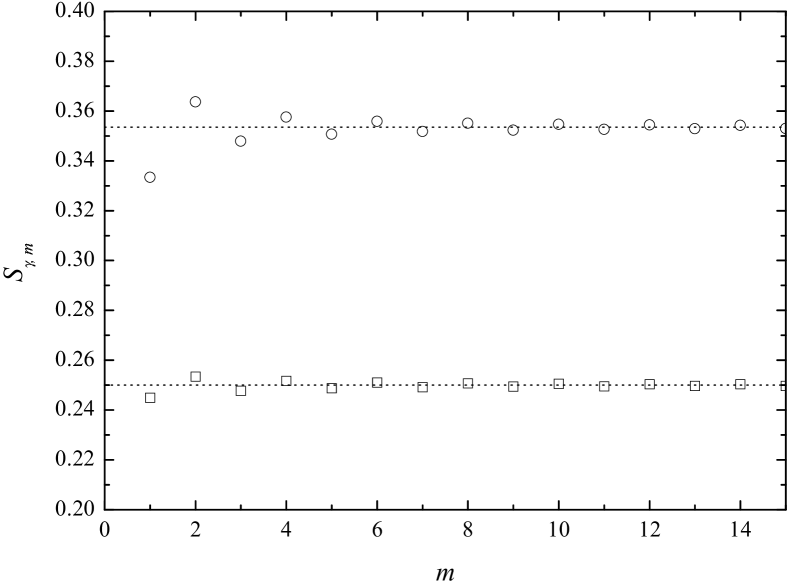
Figure 1: First values of $S_{\gamma,m}$ versus $m$ for $\gamma=1/2$ when the first-order coefficients (circles) and second-order coefficients (squares) are used. The lines mark the corresponding limit values $S_{\gamma}^{\times}$ given by Eqs. (18) and (19)

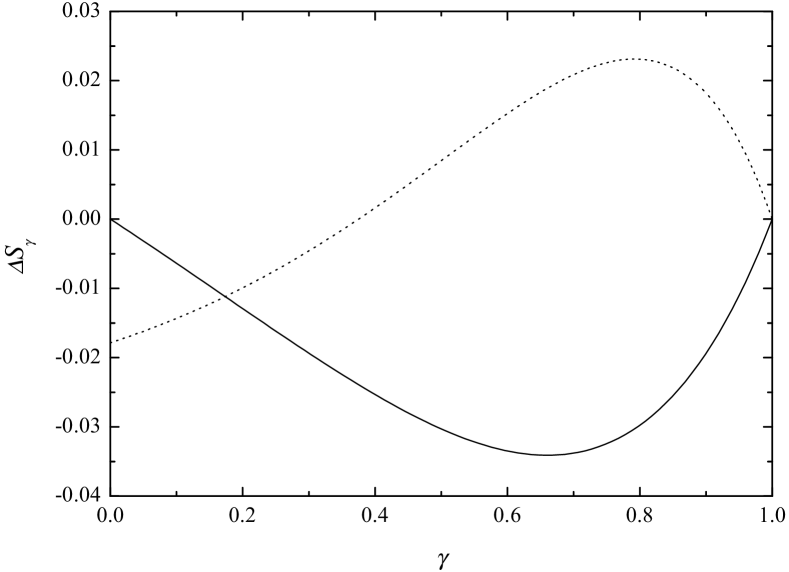
Figure 2: The difference $\Delta S_{\gamma}=S_{\gamma,2}^{\times}-S_{\gamma,1}^{\times}$ versus $\gamma$ when the first-order coefficients for $\omega_{k}^{(1-\gamma)}$ [c.f. Eq. (7)] (solid line) and second-order coefficients [c.f. Eq. (8)] (dotted line) are used.

The value of $\lim_{m\rightarrow\infty}S_{\gamma,m}^{\times}=S_{\gamma}^{\times}$ can be deduced from Eq. (17) taking into account that the coefficients $\omega_{k}^{(1-\gamma)}$ are generated by the functions given in Eqs. (6) and (8). When the first-order coefficients given by (6) are used, one gets:

$$S_{\gamma}^{\times}=\frac{1}{\left.2(1-\xi)^{1-\gamma}\right|_{\xi\rightarrow-1}}=\frac{1}{2^{2-\gamma}}\;.$$ (18)

Similarly, when the second-order coefficients given by (8) are used, one gets:

$$S_{\gamma}^{\times}=\frac{1}{\left.2\left(\frac{3}{2}-2\xi+\frac{1}{2}\xi^{2}\right)^{1-\gamma}\right|_{\xi\rightarrow-1}}=\frac{1}{4^{3/2-\gamma}}.$$ (19)

We will verify numerically in Sec. 4 that the explicit integration method as given by Eq. (11) is stable when

$$S_{\gamma}\leq\frac{S_{\gamma}^{\times}}{\sin^{2}\left(\frac{q\Delta x}{2}\right)}$$ (20)

and unstable otherwise. As the maximum value of the square of the sine function is bounded by 1, we can give a more conservative but simpler bound: the fractional FTCS method will be stable when

$$S_{\gamma}=K_{\gamma}\frac{\Delta t^{\gamma}}{(\Delta x)^{2}}\leq{S_{\gamma}^{\times}}.$$ (21)

The physical interpretation of this restriction is the same as for the diffusive case, namely, Eq. (21) means that the maximum allowed time step $\Delta t$ is, up to a numerical factor, the (sub)diffusion time across a distance of length $\Delta x$ [c.f. Eq. (1)].

Notice that the value of $S_{\gamma}^{\times}=1/4^{3/2-\gamma}$ given by Eq. (19) is smaller than $1/2^{2-\gamma}$ for any $\gamma<1$ (if $\gamma=1$ we recover the bound $S^{\times}=1/2$ of the usual explicit FTCS method for the ordinary diffusion equation [31, 32]). Consequently, the fractional FTCS method that uses a second-order approximation in the fractional derivative is “less robust” than the fractional FTCS method that uses the first-order coefficients $\omega_{k}^{(1-\gamma)}$. Taking into account that the two methods have the same precision (see Sec. 3.2) we note that nothing is gained by using the fractional derivative with higher precision. Therefore, in practical applications, we will only use here the first-order coefficients (7).

3.2 Truncating error of the fractional FTCS method

The truncating error $T(x,t)$ of the fractional FTCS difference scheme is [see (10)]:

$$T(x,t)=\frac{u_{j}^{(m+1)}-u_{j}^{(m)}}{\Delta t}-K_{\gamma}\,D_{t}^{1-\gamma}\left[\frac{{u}_{j-1}^{(m)}-2{u}_{j}^{(m)}+{u}_{j+1}^{(m)}}{(\Delta x)^{2}}\right]\;.$$ (22)

But

$$\frac{u_{j}^{(m+1)}-u_{j}^{(m)}}{\Delta t}=u_{t}+\frac{1}{2}u_{tt}\Delta t+O(\Delta t)^{2}$$ (23)

and

$$~{}_{0}D_{t}^{1-\gamma}\left[{{u}_{j-1}^{(m)}-2{u}_{j}^{(m)}+{u}_{j+1}^{(m)}}\right]=\displaystyle\frac{1}{h^{1-\gamma}}\sum_{k=0}^{m}w_{k}^{1-\gamma}\left[u_{xx}+\displaystyle\frac{1}{12}u_{xxxx}\left(\Delta x\right)^{2}+\cdots\right]+{O}\left(h^{p}\right)\;$$ (24)

so that, taking into account that $u(x,t)$ is the exact solution of Eq. (2), we finally get from Eqs. (22), (23) and (24) the following result

$$T(x,t) ={O}(h^{p})+\frac{1}{2}u_{tt}\Delta t-\frac{K_{\gamma}(\Delta x)^{2}}{12}~{}_{0}D_{t}^{1-\gamma}u_{xxxx}+\cdots$$ (25)

$$={O}(h^{p})+{O}(\Delta t)+{O}(\Delta x)^{2}\;.$$ (26)

Therefore, (i) assuming that the initial boundary data for $u$ are consistent (as assumed for the usual FTCS method [31]) and (ii) assuming that $u$ is sufficiently smooth at the origin $t=0$ [see remark below Eq. (8)], we conclude that the method discussed in this paper is unconditionally consistent for any order $p$ because $T(x,t)\rightarrow 0$ as $h$, $\Delta t$, $\Delta x\rightarrow 0$. As remarked above, in practical calculations is convenient to use $h=\Delta t$ so that, due to the term ${O}(\Delta t)$ in (26), no improvements are achieved by considering higher orders than $p=1$ in the fractional derivative. In is interesting to note that for the diffusion equation ($\gamma=1$) it is possible to cancel out the last two terms in Eq. (25) with the choice $\Delta t=(\Delta x)^{2}/(6K_{\gamma})$, trhereby obtaining a scheme that is “second-order accurate” [31]. This is not possible for the fractional case because of the fractional operator.

4 Numerical solutions and the stability bound on $S_{\gamma}$

The objective of this section is twofold: first we want to test the reliability of the numerical algorithm defined in Eq. (11) by applying it to two fractional problems with known exact solutions, and second we want to check the stability bounds obtained in Sec. 3.1.

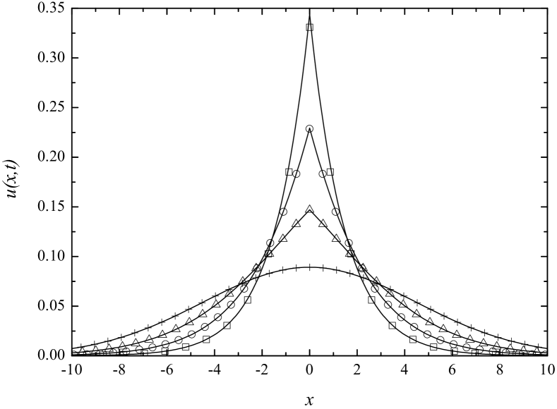
Figure 3: Comparison between the exact subdiffusion propagator (lines) and the numerical integration results for $\gamma=1/4$ (squares), $\gamma=1/2$ (circles), $\gamma=3/4$ (triangles) and $\gamma=1$ (crosses) and $t=10$.

4.1 Numerical solution versus exact solution: two examples

The fundamental solution of the subdiffusion equation in Eq. (2) corresponds to the problem defined in the unbounded space where the initial condition is $u(x,t=0)=\delta(x)$. This solution is called the propagator (or Green’s function) and can be expressed in terms of Fox’s H-function [7]:

$$u(x,t)=\frac{1}{\sqrt{4\pi K_{\gamma}t^{\gamma}}}\,H^{10}_{11}\left[\frac{|x|}{\sqrt{K_{\gamma}t^{\gamma}}}\left|\begin{array}[]{l}{(1-\gamma/2,\gamma/2)}\\[4.30554pt] {(0,1)}\end{array}\right.\right]\;.$$ (27)

In our numerical solution we used the boundary conditions $u(-L,t)=u(L,t)=0$ with a sufficiently large $L$ in order to avoid finite size effects. In Fig. 3 we compare the numerical integration results with the exact solution (27) for $\gamma=1/4$, $1/2$, $3/4$, $1$ at $t=10$. The timestep used was $\Delta t=0.01$ and $\Delta x=\sqrt{K_{\gamma}(\Delta t)^{\gamma}/S_{\gamma}}$ with $K_{\gamma}=1$ and $S_{\gamma}=0.28$, $0.33$, $0.4$ and $0.5$. All these values of $S_{\gamma}$ are just below the stability bound $S_{\gamma}^{\times}$ (see Eq. (18)). The agreement is excellent except for $\gamma=1/4$ and $x=0$, but this minor discrepancy is surely due to the large spatial cell $\Delta x\simeq 1.06$ used in this case.

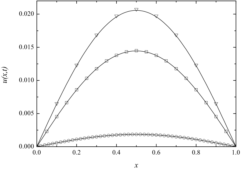
Figure 4: Numerical solution of the subdiffusion equation for the problem with absorbing boundary conditions, $u(0,t)=u(1,t)=0$, and initial condition $u(x,0)=x(1-x)$ versus the exact analytical result (lines) for $t=0.5$. The solution $u(x,t)$ is shown for $\gamma=0.5$ (triangles), $\gamma=0.75$ (squares) and $\gamma=1$ (circles).

We have also considered a problem with absorbing boundaries, $u(0,t)=u(1,t)=0$, and initial condition $u(x,t=0)=x(1-x)$. The exact analytical solution of Eq. (2) is easily found by the method of separation of variables: $u(x,t)=X(x)T(t)$. We thus find $X_{n}(x)=\sin(n\pi x)$ and

$$\frac{dT}{dt}=-K_{\gamma}\,\lambda_{n}^{2}~{}_{0}D_{t}^{1-\gamma}T\;,$$ (28)

where $\lambda_{n}=n\pi$, $n=1,2,\ldots$. The solution of Eq. (28) is found in terms of the Mittag-Leffler function [7]:

$$T_{n}(t)=E_{\gamma}(-K_{\gamma}n^{2}\pi^{2}t^{\gamma})\;.$$ (29)

Imposing the initial condition we obtain

$$u(x,t)=\frac{8}{\pi^{3}}\sum_{n=0}^{\infty}\frac{1}{(2n+1)^{3}}\sin[(2n+1)\pi x]E_{\gamma}[-K(2n+1)^{2}\pi^{2}t^{\gamma}]\;.$$ (30)

In Fig. 4 we compare this exact solution with the results of the numerical integration scheme for $\gamma=0.5$, $\gamma=0.75$, and $\gamma=1$ for $t=0.5$ and $K_{\gamma}=1$. The values of $S_{\gamma}$ used were $S_{\gamma}=0.33$, $0.4$, and $0.5$ with $\Delta x=1/10$, $1/20$, and $1/50$, respectively. The values of $\Delta t$ for fixed $S_{\gamma}$ and $\Delta x$ stem from the definition of $S_{\gamma}$:

$$\Delta t=\left[\frac{S_{\gamma}(\Delta x)^{2}}{K_{\gamma}}\right]^{1/\gamma}\;.$$ (31)

Excellent agreement is observed for the three values of $\gamma$, it being slightly poorer for the smallest value which is not surprising because in this case the mesh size $\Delta x=1/10$ used is the largest.

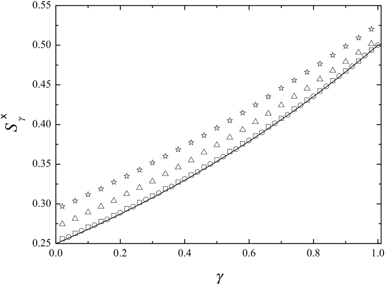
Figure 5: Values of $S_{\gamma}^{\times}$ corresponding to the onset of instability versus the subdiffusion exponent $\gamma$. The solid line is the prediction of the Fourier–von Neumann analysis and the symbols denote the results of the numerical tests with the criterion in Eq. (32): stars, triangles and squares for the absorbing boundary problem with $u(x,0)=x(1-x)$ with $M=50$, $100$ and $1000$, respectively, and circles for the propagator with $M=1000$.

4.2 Numerical check of the stability analysis

We checked the stability bound on the value of the $S_{\gamma}$ given in Eq. (18) in the following way. For a set of values of $\gamma$ in the interval $[0,1]$, and for values of $S_{\gamma}$ starting at $S_{\gamma}=0.98S_{\gamma}^{\times}$ (in particular, for $S_{\gamma}=0.98/2^{2-\gamma}+0.001\,n$, $n=0,1,2,\ldots$) we applied the fractional FTCS integration until step $M$. We say that the resulting integration for a given values of $\gamma$ and $S_{\gamma}$ is unstable when the following condition is satisfied at any position $j$:

$$\left|\frac{u_{j}^{m-1}}{u_{j}^{m}}-\Xi\right|>\Xi\quad\text{for any}\quad m=M-\Delta M,M-\Delta M+1,\ldots,M\;,$$ (32)

where $\Xi=5$ and $\Delta M=10$. This means that the numerical solution is considered unstable if the quotient $u_{j}^{m-1}/u_{j}^{m}$ becomes negative or larger than $2\Xi$ at any of the last $\Delta M$ steps. (Of course, this criterion is arbitrary; however, the results do not change substantially for any other reasonable choice of $\Xi$ and $\Delta M$.) Let $S_{\gamma}^{\text{min}}$ be the smallest value of $S_{\gamma}=0.98/2^{2-\gamma}+0.001\,n$ that verifies the criterion (32). For the absorbing boundary problem we calculate these values using $\Delta x=1/2N$ with $N=5$ and $M=50$, $M=100$ and $M=1000$. For the propagator, we calculate $S_{\gamma}^{\text{min}}$ using $M=1000$ and $\Delta t=5\times 10^{-4}$ in a lattice with absorbing frontiers placed at $x=-N\Delta x$ and $x=N\Delta x$ with $N=50$. It is well known that for a lattice with $2N+1$ points (including the absorbing boundaries) the maximum value of $\sin(q\Delta x/2)$ in Eq. (17) occurs for $q\Delta x=(2N-1)\pi/(2N)$, so that in Fig. (5) we plot $S_{\gamma}^{\text{min}}\sin^{2}[(2N-1)\pi/(4N)]$. We observe that for large $M$ the stability bound predicted by Eq. (18) agrees with the result of the numerical test. The larger values obtained for smaller $M$ mean that the method must be “very unstable” to fulfill our instability criterion in so few steps. The success of the numerical test is truly remarkable and supports the unorthodox application of the Fourier–von Neumann stability analysis to the fractional FTCS scheme made in Sec. 3.1.

In Fig. (6) we plot the numerical solution when $S_{\gamma}=0.36>S_{\gamma}^{\times}$ in the case of the propagator with $\gamma=1/2$. This kind of oscillatory behaviour in the unstable domain is typical for ordinary partial differential equations too.

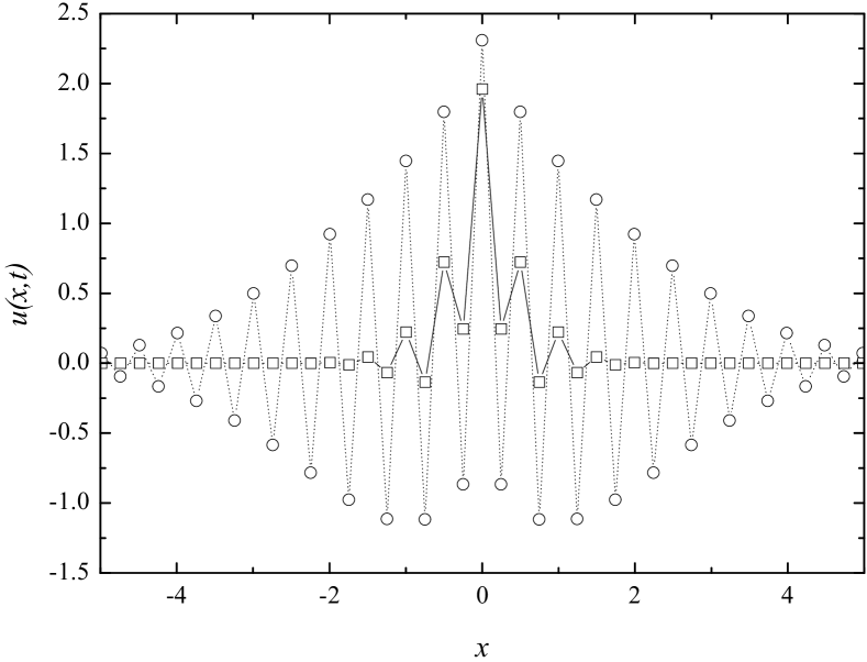
Figure 6: The propagator $u(x,t)$ for $\gamma=1/2$, $K_{\gamma}=1$, $S=0.36$ and $t=0.005$ (squares) and $t=0.05$ (circles). The time step is $\Delta t=0.0005$ and the spatial mesh $\Delta x$ is obtained according to Eq. (31). The lines are plotted as a visual guide.

5 Concluding remarks

The availability of efficient numerical algorithms for the integration of fractional equations is important as these equations are becoming essential tools for the description of a wide range of systems [6]. In this paper we have discussed a numerical algorithm for the solution of the fractional (sub)diffusion equation (2). Although we have dealt with this particular equation, our procedure could be extended to any fractional integro-differential equation by means of an obvious combination of the Grünwald-Letnikov definition of the fractional derivative [1, 2, 7] with standard discretization algorithms used in the context of ordinary partial differential equations [31]. Furthermore, the method (given its explicit nature) can be trivially extended to $d$-dimensional problems, which is not such an easy task when implicit methods are considered.

In our numerical method the state of the system at a given time $t=m\Delta t$ is given explicitly in terms of the previous states at $t=(m-1)\Delta t,\ldots,\Delta t,0$ by means of the FTCS scheme (11). We verified that for some standard initial conditions with exact analytical solution, namely, (a) the propagator in an unlimited system with $u(x,t=0)=\delta(x)$ and (b) a system with absorbing boundaries and $u(x,t=0)=x(1-x)$, the present algorithm leads to numerical solutions which are in excellent agreement with the exact solutions. Using a Fourier–von Neumann technique we have provided the conditions for which the fractional FTCS method is stable. For example, if a first-order approximation for the fractional derivative is considered, we have shown that the FTCS algorithm is stable if $S_{\gamma}=K_{\gamma}(\Delta t)^{\gamma}/(\Delta x)^{2}\leq 1/2^{2-\gamma}$. For $\gamma=1$ the well-known bound $S=D\Delta t/(\Delta x)^{2}\leq 1/2$ of the ordinary explicit method for the diffusion equation is recovered.

Concerning the implementation of the method we must remark that the evaluation of the state of the system at a given time step $m\Delta t$ requires information about all previous states at $t=(m-1)\Delta t,(m-2)\Delta t,\ldots,\Delta t,0$ and not merely the immediately preceding one as occurs in ordinary diffusion. This is a consequence of the non-Markovian nature of subdiffusion and implies the need for massive computer memory in order to store the evolution of the system, which is especially cumbersome in computations of long-time asymptotic behaviours. This could be palliated by using the “short-memory” principle [1]. Another feature of the explicit numerical scheme is the interdependence of the temporal and spatial discrete steps for a fixed $S_{\gamma}$. If, as usual, one intends to integrate an equation with a given mesh $\Delta x$, then the corresponding step size $\Delta t$ for a given $S_{\gamma}<S_{\gamma}^{\times}$ is of the order $(\Delta x)^{2/\gamma}$. As a consequence, $\Delta t$ could become extremely small even for no too small values of $\Delta x$, especially when the problem is far from the diffusion limit, i.e., for small values of $\gamma$, so that the number of steps needed to reach even moderate times would become prohibitively large. In this case, the resort to implicit methods [18, 25, 26, 27, 28, 29, 30], stable for any value of $\Delta t$ and $\Delta x$, is compulsory.

This work has been supported by the Ministerio de Ciencia y Tecnología (Spain) through Grant No. BFM2001-0718.

References

- [1] I. Podlubny, Fractional Differential Equations, (Academic Press, San Diego, 1999).
- [2] R. Hilfer, Ed., Applications of Fractional Calculus in Physics, (World Scientific, Singapore, 2000).
- [3] J. W. Kirchner, X. Feng and C. Neal, Nature 403 (2000) 524.
- [4] H. Scher, G. Margolin, R. Metzler and J. Klafter, Geophysical Research Letters 29 (5) (2002) doi:10.1029/2001GL014123.
- [5] B. Berkowitz, J. Klafter, R. Metzler and H. Scher, preprint cond-mat/0202327 v2 (2002).
- [6] I. M. Sokolov, J. Klafter and A. Blumen, Physics Today 55 (11)(2002) 48.
- [7] R. Metzler, J. Klafter, Phys. Rep. 339 (2000) 1.
- [8] G. Rangarajan and M. Ding, Phys. Lett. A 273 (2000) 322; Phys. Rev. E 62 (2000) 120.
- [9] B. H. Hughes, Random Walks and Random Environments, Volume 1: Random Walks (Oxford, Clarendon Press, 1995); Random Walks and Random Environments, Volume 2: Random Environments (Oxford, Clarendon Press, 1995).
- [10] V. Balakrishnan, Physica A 132 (1985) 569.
- [11] W. Wyss, J. Math. Phys. 27 (1986) 2782.
- [12] W. R. Schneider and W. Wyss, J. Math. Phys. 30 (1989) 134.
- [13] R. Metzler, E. Barkai and J. Klafter, Phys. Rev. Lett. 82 (1999) 3563.
- [14] A. Compte, Phys. Rev. E 55 (1997) 6821.
- [15] A. Compte and M. O. Cáceres, Phys. Rev. Lett. 81 (1998) 3140.
- [16] R. Metzler, J. Klafter and I. M. Sokolov, Phys. Rev. E 58 (1998) 1621.
- [17] S. B. Yuste and K. Lindenberg, Phys. Rev. Lett. 87 (2001) 118301; Chem. Phys. 284 (2002) 169.
- [18] C. Chuanmiao and S. Tsimin, Finite Element Methods for Integrodifferential Equations (World Scientific, Singapore, 1998).
- [19] R. Metzler and J. Klafter, Physica A 278 (2000) 107.
- [20] E. Baraki and R. J. Silbey, J. Phys. Chem. B 104 (2000) 3866.
- [21] I. M. Sokolov, preprint cond-mat/0101232 (2001).
- [22] R. Gorenflo and F. Mainardi, Fract. Calculus Appl. Anal. 1 (1998) 167.
- [23] R. Gorenflo, G. De Frabritiis and F. Mainardi, Physica A 269 (1999) 79.
- [24] R. Gorenflo, F. Mainardi, D. Moretti, G. Pagnini and P. Paradisi, Chem. Phys. 284 (2002) 521.
- [25] J. M. Sanz-Serna, SIAM J. Numer. Anal. 25 (2002) 319.
- [26] J. C. L pez-Marcos, SIAM J. Numer. Anal. 27 (2002) 20.
- [27] CH. Lubich, I. H. Sloan, and V. Thom e, Math. Comp. 65 (1996) 1.
- [28] W. McLean and V. Thom e, J. Austral. Math. Soc. Ser. B 35 (1993) 23.
- [29] W. McLean, V. Thom e and L. B. Wahlbin, J. Comp. Appl. Math. 69 (1996) 49.
- [30] K. Adolfsson, M. Enelund and S. Larsson (preprint avaliable at http://www.math.chalmers.se/stig/papers/adap.pdf)
- [31] K. W. Morton and D. F. Mayers, Numerical Solution of Partial Differential Equations, (Cambridge University Press, Cambridge, 1994).
- [32] W. H. Press, S. A. Teukolsky, W. T. Vetterling and B. P. Flannery, Numerical Recipes in Fortran 77: The Art of Scientific Computing (second edition) (Cambridge University Press, Cambridge, 1992).
- [33] Ch. Lubich, SIAM J. Math. Anal. 17 (1986) 704.
- [34] R. Gorenflo, in: Fractals and Fractional Calculus in Continuum Mechanics, eds. A. Carpinteri and F. Mainardi (Springer Verlag, New York, 1997) p. 277.