Modeling State in Software Debugging of VHDL-RTL Designs – A Model-Based Diagnosis Approach

Abstract

In this paper we outline an approach of applying model-based diagnosis to the field of automatic software debugging of hardware designs. We present our value-level model for debugging VHDL-RTL designs and show how to localize the erroneous component responsible for an observed misbehavior. Furthermore, we discuss an extension of our model that supports the debugging of sequential circuits, not only at a given point in time, but also allows for considering the temporal behavior of VHDL-RTL designs. The introduced model is capable of handling state inherently present in every sequential circuit. The principal applicability of the new model is outlined briefly and we use industrial-sized real world examples from the ISCAS’85 benchmark suite to discuss the scalability of our approach.

0309027197

Bernhard Peischl and Franz WotawaModeling State in Software Debugging of VHDL-RTL Designs – A Model-Based Diagnosis Approach

1 Technische Universit”at Graz, Institute for Software Technology (IST), Inffeldgasse 16b/2, A-8010 Graz, Austria, {peischl,wotawa}@ist.tu-graz.ac.at

1Authors are listed in alphabetical order.

1 Introduction

During the last decade, hardware description languages like Verilog and VHDL (Very High Speed Integrated Circuit Hardware Description Language) have become common for designing circuits. In order to reduce time to market, which becomes increasingly important in today’s fast paced economy, applying formal verification techniques and extensive simulation is imperative in order to master the error-prone development process of complex circuit designs. However, if some faulty behavior is identified due to simulation or automated verification, the location of the error in the source code is of particular interest. Nevertheless, there is currently almost no support for the designer in fixing the faults thus found. Traditional debuggers force the developer to go through the code and therefore fault localization and error correction is a time consuming task.

To overcome these issues several approaches for automated fault localization have been proposed including program-slicing Wei (82, 84), algorithmic debugging Sha (83), dependency-based techniques Kup (89); Kor (88); Jac (95) and probability-based methods BH (93). Moreover, in the recent years, the usage of model-based diagnosis Rei (87); dKW (87); GSW (89) for debugging software has been examined in a wider context FSW (99); MSW (99); SW (99). All of these approaches have in common that they use a model that can be automatically derived from the source code, they use different abstractions and also differ in the programming languages being considered. The spectrum ranges from purely logical languages to imperative languages and hardware description languages such as VHDL.

In this paper we focus on software debugging of hardware designs, particularly on our modeling approach for VHDL programs. By using a domain-independent diagnosis engine together with a specific model abstracting syntax and semantics of the programming language, this approach allows for automated debugging of logical, imperative FSW (99); MSW (99) and functional programming languages SW (99) . By changing the underlying model the approach can be tailored to specific programming languages without the need for changing the underlying algorithm for fault localization.

In this paper we present an extension to previous research Wot (00, 02) on debugging VHDL designs by introducing a model extension that allows not only for fault localization at a given point in time but also allows for considering the temporal behavior of a VHDL program. The new model improves the previous model in that it explicitly captures process semantics by unfolding process executions over time and allows for representing the state of sequential circuit designs. This is done by unfolding the model in time and by creating temporal instances of components for every possible process execution.

The remainder of the paper is organized as follows. The next section outlines the main ideas behind model-based diagnosis. Section 2 applies model-based diagnosis to localize faults in VHDL programs by presenting a small but realistic example. We use a 2-bit counter to show our modeling approach for a single point in time. Section 3 introduces our new model extension that allows for considering the temporal behavior of the design rather than using a single point in time and Section 4 outlines some empirical results obtained from real-world examples. An overview summarizing the paper’s main contribution and a discussion on related and forthcoming research concludes the paper.

1.1 Model-Based Diagnosis and Software Debugging

The basic idea of model-based diagnosis is to use knowledge of the correct behavior of the components of a system together with knowledge of the structure of the system to locate the cause of the misbehavior. The behavior and the structure of the system are the model and the components of the system are the parts that behave either correct or abnormal.

A model-based diagnosis engine assumes that some components are faulty and the remaining ones are not. This approach requires a specification of the correct behavior of the components but it does not require knowledge about the behavior of a faulty component. The diagnosis engine checks whether the model contradicts some given observations under certain assumptions about the abnormality of components. If there is no contradiction, then the assumption is justified and the assumed faulty components are a valid diagnosis of the given system.

The crucial decision when building a diagnosis model from program code involves the choice of those parts of the program which are represented as components in the model. This decision directly influences the granularity of the diagnosis results. For example, if statements are mapped to components, bugs can only be localized on the statement level. Faults inside a statement cannot be diagnosed without fault models, that is, knowledge about how a particular type of fault may change the system’s behavior. Using expressions as diagnosis components allows finer granularity at the cost of increasing the number of components and thus the overall diagnosis time increases considerably.

Using the consistency-based view on diagnosis as defined by Rei (87), a diagnosis system can be formally stated as a tuple $(SD,COMP)$ where $SD$ (system description) is a logical theory modeling the behavior of the given program to be debugged, and $COMP$ is a set of components, i.e., statements or expressions. A diagnosis system together with a set of observations $OBS$, that is, a test case, forms a diagnosis problem. A diagnosis $\Delta$ is a subset of $COMP$, with the property that the assumption that all components in $\Delta$ are abnormal (they do not behave as expected), and the rest of the components is behaving normal (they behave as expected), is required to be consistent with $SD$ and $OBS$. Formally, $\Delta$ is a diagnosis if and only if $SD\cup OBS\cup\{\neg AB(C)|C\in COMP\setminus\Delta\}\cup\{AB(C)|C\in\Delta\}$ is consistent, where $\neg AB(C)$ formalizes a correctly operating component. Note, that in contrast to correctness, which in the terminology of software engineering requires that there is no contradiction taking into account all test cases, the notion of consistency in the context of model-based diagnosis refers to logical validity with respect to a given test case under a given set of assumptions.

The basis for localizing faults is that an incorrect output value (where the incorrectness can be observed directly or derived from observations of other signals) cannot be produced by a correctly functioning component with correct inputs. Therefore, to make a system with observed incorrect behavior consistent with the description, some subset of its components has to be assumed to work incorrectly. In practical terms, one is interested in finding minimal diagnosis, i.e., a minimal set of components whose malfunction explains the misbehavior of the system.

In principle all diagnoses can be computed by successively testing all subsets of $COMP$ . However, in automated debugging this approach can only be applied for rather small programs and is not feasible for industrial sized designs. Reiter Rei (87) proposed the use conflicts. A set $CO\subseteq COMP$ is a conflict if and only if $SD\cup OBS\cup\{\neg AB(C)|C\in CO\}$ is contradictory, i.e., assuming that the statements in $CO$ are abnormal leads to inconsistency. The relationship between diagnosis and conflicts can be explained as follows. A conflict states that $\neg AB(C_{1})\wedge\neg AB(C_{2})\wedge...\wedge\neg AB(C_{n})$ contradicts the observation. In order to resolve the contradiction at least one of the assumptions $\neg AB(C_{1}),...\neg AB(C_{n})$ has to be false, i.e., there must be a $C_{i}$; $0\leq i\leq n$ where $AB(C_{i})$ is true. If we want to resolve all conflicts we have to choose one (not necessarily different) element from every conflict. Since the so chosen elements resolve all conflicts, they must form a diagnosis.

A set with the property that the intersection with all elements of a set of sets is not empty is called a hitting set. Hence, a minimal diagnosis (a diagnosis where no subset is a diagnosis) is a minimal hitting set of (not necessarily minimal) conflicts. From this observation follows that there exists only a single- diagnosis (a diagnosis with exactly one component) if and only if the component is element of every conflict. Reiter Rei (87) proposed an algorithm to compute all minimal diagnoses from the conflicts by means of a so called hitting set tree. There are algorithms where this process is done in an iterative fashion, that is, conflicts are computed on demand. Although computing all conflicts is of order $2^{|COMP|}$ the computation of single conflicts (which are not minimal) can be done in linear time when assuming the the model is written as a set of propositional Horn clauses. Alternatively, there are other very fast diagnosis algorithms that rely on other principles SW (97); FD (95).

2 Debugging of VHDL-RTL-Programs

In the domain of debugging hardware designs the model is given by the syntax of the program and the semantics of the language, which in our case is the RTL subset (Register Transfer Level) of VHDL. Depending on the required granularity, components refer to statements or expressions. In the following we present an introductory example in which we assume that statements correspond to diagnosis components. Hence, statements are the smallest parts of the program that can be either correct of faulty.

Figure 1 outlines the VHDL code of a 2 bit counter that decrements its value if the input $E1$ is set to 1 and $E2$ is set to 0; if both inputs are set to 0 the counter increments its value whenever a rising edge occurs on the $CLK$ signal. If $E1$ is set to 0 and $E2$ is set to 1 the counter is reset to 0, and finally, if both inputs are 1 the counter is set to value 3. The output of the counter is coded using a 1-from-4 encoder. The value 0 is thus represented by $A1A2A3A4=1000$ whereas the value 3 is coded by $A1A2A3A4=0001$.

The behavior of our program can be compiled into a simple state-transition diagram, outlined in Figure 2. There the values of the signals $Q1$ and $Q2$ are given in circles (as states of the automaton), and the inputs and corresponding outputs are given on the arcs (encoded as $E1E2/A1A2A3A4$). The initial state is indicated by an arrow.

entity COUNTER is
  port(
    E1, E2, CLK    : in  bit;
    A1, A2, A3, A4 : out bit);
   end COUNTER ;

    architecture BEHAV of COUNTER is
      signal D1, D2, Q1, Q2, NQ1, NQ2 : bit := 0;
    begin
       comb_in : process (Q1, Q2, E1, E2)
         variable I1, I2 : bit;
       begin
         I1 := not((Q1 and Q2) or (not(Q1) and not(Q2)));
         I2 := (I1 and E1) or (not(I1) and not(E1));
         D1 <= (E1 and E2) or (E2 nor I2);
         D2 <= (E1 and E2) or (E2 nor Q2);
       end process comb_in;

       comb_out : process (Q1, Q2, NQ1, NQ2)
       begin
          A1 <= NQ2 and NQ1;
          A2 <= Q2 and NQ1;
          A3 <= NQ2 and Q1;
          A4 <= Q1 and Q2;
       end process comb_out;


        p1:process (Q1)
        begin
                NQ1 <=  not(Q1);
        end process p1;

        p2:process(Q2)
        begin
                NQ2 <= not(Q2);
        end process p2;

       dff : process (CLK)
       begin
         if (CLK = ’1’) then
           Q1 <= D1;
           Q2 <= D2;
         end if;
       end process dff;
    end BEHAV;

Figure 1: The source code of the 2-bit counter.

Figure 2: The state-transition diagram.

In order to state the idea of applying model-based diagnosis to locate the cause of an observed misbehavior we introduce a bug into the program by simply omitting the not operator in line 30:

p1:process (Q1) begin NQ1 ¡= Q1; end process p1;

Figure 3: The state-transition diagram of the faulty program.

The state transition diagram of the erroneous program is given in Figure 3. Considering this diagram, it is obvious that our design contains a bug: Since the counter uses a 1 from 4 coded output, exactly one of the outputs should be 1 at any time, and this is not the case. From the failed property we can identify the temporal context and retrieve the relevant state of the observed misbehavior. Note that this can be done either manually by an experienced designer or by means of automated verification techniques such as model checking. By using the values of the retrieved state, the input signals and the erroneous output signals at a specific point in time as observations we can use model-based diagnosis to search for faulty statements that explain the observed misbehavior.

Figure 4: The structural model of the counter.

In order to locate the bug in the program, we have to build a model of the program which comprises the structure and the behavior of the counter. The structural part can be obtained by viewing statements as diagnosis components and signals and variables as connections between them. For VHDL some semantic aspects have to be considered, e.g., the different handling of variables and signals. However, for sake of brevity we do not discuss these issues in this article. Details can be found in Wot (00, 02). Figure 4 shows the structural part of the model where components (statements in our case) are indicated using boxes.

The description of the components’ behavior remains to be introduced. The component model itself can be derived directly from the associated statements. For example, the correct behavior of the if-then-else statement can be represented by logical sentences. The output of an if-then-else statement is determined by so called sub-blocks, that represent the statements in the if and the else branch, respectively. If the component works as expected, that is, $\neg AB(IF)$ is assumed to be true, and the condition evaluates to true, the then sub-block, associated with the statements in the if branch, is transferred to the output. Otherwise the evaluated sub-block representing the else branch is assigned to the output. In formal terms this can be expressed as follows:

$$\forall x\in stmts_{then}\cdot\neg AB(IF)\wedge(cond(IF)=true)\rightarrow(out_{x}(IF)=in_{then}(IF))$$

$$\forall x\in stmts_{else}\cdot\neg AB(IF)\wedge(cond(IF)=false)\rightarrow(out_{x}(IF)=in_{else}(IF))$$

In the formal model outlined above $stmts_{then}$ denotes the signal assignment-statements in the if-branch, $stmts_{else}$ represents the statements in the else-branch and the signal $out_{x}$ denotes a single output $x$. Similar models can be introduced for all the other components in the example. Details of modeling other VHDL-RTL language artefacts can for example be found in Wot (02).

For locating the fault in our program automatically, we make use of the available knowledge about the values of the signals. For our example we consider the detected misbehavior for the case of counting downwards ($E1=1$, $E2=0$). According to the state-transition diagram in Figure 3 the misbehavior is encountered several times. However, retrieving an appropriate state for computing diagnoses is in the responsibility of the designer. From the failed property we know that the program behaves wrong if $CLK=1$, $E1=1$, $E2=0$, $Q1=1$ and $Q2=0$. We now take the expected output values and the values from the state-transition diagram of the erroneous program to identify the conflicts. Note that the values of $Q1$ and $Q2$ are known for two successive states, hence we are able to eliminate the circular structure in Figure 4.

According to the transition-diagram of the correct program, we expect the values $A1A2A3A4=0010$ rather than the produced output $A1A2A3A4=1010$ for the given input signals. Thus, recalling the definition of conflicts, we obtain two conflicts: One conflict comprises the statements $\{NQ1<=Q1$, $NQ2<=not(Q2)$, $A1<=NQ2$ $and$ $NQ1$}, and the other one consists of $\{NQ1<=Q1$, $A3<=NQ2$ $and$ $Q1$, $A1<=NQ2$ and $NQ1$}. Figure 5 outlines the computation of the conflicts graphically.

Figure 5: The computation of the conflicts in the counter model.

Using these conflicts we can compute diagnoses by employing a hitting set tree. In general, we have to built a directed acyclic graph GSW (89), but in our special case we simply obtain a tree. Our hitting set tree, called $T$ in the following, is a smallest edge-labeled and node-labeled tree with the following properties Rei (87); GSW (89):

• The root of the tree is labeled by an arbitrary conflict.

• For each node $n$ of $T$, let $H(n)$ denote the set of edge-labels on the path in $T$ from the root node to $n$. The label for $n$ is any conflict $CO$ such that $CO\cap H(n)=\{\}$, if such a conflict exists. Otherwise the label for node $n$ is $\surd$. If $n$ is labeled by the set $CO$, then for each $\sigma\in CO$, $n$ has a successor, $n_{\sigma}$, joined to $n$ by an edge labeled by $\sigma$.

Figure 6: The hitting set tree for the conflicts of the counter.

Figure 6 outlines the hitting set tree for the conflicts we obtained from our example. By collecting the edge-labels from the leaves marked with $\surd$ up to the root in a focused breath-first search order all minimal diagnoses can be retrieved from the hitting-set tree efficiently.

For example, considering the first level of the tree we obtain the statements {$A1<=NQ2$ $and$ $NQ1$} and {$NQ1<=Q1$} (the introduced bug) as single-fault diagnoses. Furthermore, taking into account the next level of the hitting-set tree, there is a single dual-fault diagnosis : $\{NQ2<=NOT(Q2),A3<=NQ2$ $and$ $Q1$}. The remaining diagnoses at this level can be ruled out; they do not represent minimal diagnosis because a proper subset is already known as a single-fault diagnosis. Usually, we prefer single-fault diagnoses, since they are more probable. However, note that although {$A1<=NQ2$} is the real cause of the misbehavior, a correct behavior for the given test case can also be obtained by appropriately modifying all statements of one of the the remaining diagnoses.

3 Using Temporal Abstraction For Fault Localization

In the following we present a model extension that allows not only for localizing a fault at a given point in time, but also exploits the temporal behavior of a circuit. The model extension is put on top of the model introduced previously and allows for representing state explicitly but still can be used with a standard diagnosis engine. As in the previous section, we first introduce the structure of the new model and afterwards outline the behavioral description of the components. When dealing with temporal aspects of VHDL-RTL designs it is reasonable to require some restrictions.

For our research prototype we required that signal-assignment statements do not contain a VHDL after clause. Processes are required to have an explicit sensitivity-list and are not allowed to contain wait statements. Furthermore, we require the process activation graph to be acyclic. Thus, considering a VHDL program that comprises $n$ processes each process can at most be activated by $n-1$ other processes. Taking into account the initial activation, there is an upper bound of $n$ process activations for a single process per simulation cycle.

Simulating a program corresponds to computing all the values of the signals and variables for a ordered set of times. At a technical level, the simulation of a program is decomposed into atomic steps referred to as basic simulation cycles (BSCs). A BSC at a specific point in time $T$ and a given state $I$ of a VHDL program executes all processes for which at least one signal on which an event occurred, appears in the sensitivity-list, and updates the signal values according to the semantics of VHDL. Formally, a BSC can be expressed as a triple $(E_{T}^{I},P_{T}^{I},E_{T}^{I+1})$ where $E_{T}^{I}$ denotes the input environment and $E_{T}^{I+1}$ stands for the bindings of signals and variables to their values after executing the processes in $P_{T}^{I}$. Figure 7 outlines the way in which BSCs are connected. Note that the output environment of a certain BSC is the input environment of the succeeding one.

Figure 7: The structure of the model in terms of the introduced notations.

Furthermore, the figure outlines a so called simulation sequence, the definition of which is given in the following. A simulation sequence $\Sigma_{T}$ at time $T$ of a RTL program is a sequence of basic simulation cycles $BSC^{0}_{T},BSC^{1}_{T},\ldots,BSC^{len}_{T}$, where $len$ denotes the length of $\Sigma_{T}$. The state number of the last element of the simulation sequence is called the length of the simulation sequence $len$. In order to state the treatment of variables and signals between successive simulation sequences we have to introduce an interpretation function $E_{T}^{I}:SIG\cup VAR\mapsto VAL$ that maps signals $SIG$ and variables $VAR$ to their corresponding values $VAL$. By using this function the initial input values of a simulation sequence $\Sigma_{T_{j}}$ can be stated as follows.

$E^{0}_{T_{j}}(X)=\left\{\begin{array}[]{ll}E^{0}_{T_{j}}(X)&\mbox{ j = 0 $\vee X\in dom(E_{T_{j}}^{0})$}\\ E^{len}_{T_{j-1}}(X)&\mbox{ otherwise}\\ \end{array}\right.$

In the formula given above $X$ denotes a variable or signal and the function $dom$ retrieves the names of the signals and variables of a given environment. The formula states that the state at time point $T_{j-1}$ is used for performing the simulation at time point $T_{j}$ except from those variables and signals that are explicitly given in the input environment $E_{T_{j}}^{0}$. Note that the formalization requires an initial binding for every signal or variable $X$ in $E_{T_{0}}^{0}$. This approach allows for representing so called external signals, the values of which are given from the outside (e.g. a $CLK$ signal), in our model.

By using the terms and notations introduced above we are able to describe our diagnosis model in terms of BSCs. Formally, the system description for a simulation sequence $S_{T_{0}},S_{T_{1}},...,S_{T_{k}}$ where each $S_{T_{i}}$ is a sequence of BSCs $BSC_{T_{i}}^{0},...,BSC_{T_{i}}^{len}$ is given by the following logical sentence.

$SD=\bigcup_{T}SD(S_{T})\cup CONN,SD(S_{T})=\bigcup_{i=1}^{len(S_{T})}SD(BSC_{T}^{i})$

$SD(BSC_{T}^{i})$ is composed from the system description at a single point in time $T$ and also covers the event handling according to the VHDL semantics. Moreover, $CONN$ denotes logical sentences that describe the connection between the BSCs itself (depicted by solid lines in Figure 7) as well as BSC sequences (the corresponding connections are outlined by using a dashed line). These connectivities are given by the signals that a temporal process instance uses likewise as input and output. Using this approach our model can handle state by unfolding process executions over time. The handling of events and the logical description of a process component remains to be introduced.

VHDL designs consist of processes that are assumed to be executed in parallel and which communicate by means of signals. A process $p$ is executed if at least one of the signals that occur on its sensitivity-list has changed its value in the preceeding simulation cycle. If this is the case, the values of the signals used as a target in the sequential statement part are computed according to the VHDL semantics. If none of the signals within the sensitivity list has changed its value, then the original input values before executing the sequential statement block of process $p$ are propagated to the output of the process component. In the following a logical description of a process component $p$ is outlined:

$\forall y\in inputs(p)\cdot\exists x\in sensitivity-list(p)\cdot$

$s(x)=true\rightarrow out_{y}(p)=in_{y}(p)$

$\forall y\in inputs(p)\cdot\forall x\in sensitivity-list(p)\cdot$

$s(x)=false\rightarrow out_{y}(p)=def_{y}(p)$

$out_{y}(p)=def_{y}(p)\leftrightarrow out_{y^{\prime}EVENT}(p)=false$

$out_{y}(p)\neq def_{y}(p)\leftrightarrow out_{y^{\prime}EVENT}(p)=true$

In the logical sentences above $inputs(p)$ denotes the set of inputs of the process $p$ and $sensitivity-list(p)$ represents the sensitivity list of the process $p$. The predicate $s(x)$ is set true if signal $x$ has changed its value. The signal value $y$ after executing the sequential statement part of process $p$ is represented by $in_{y}(p)$ whereas the corresponding unmodified input of the process $p$ is represented in formal terms by $def_{y}(p)$. Furthermore, if an output has changed, the corresponding event signal is set to true.

Beside the system description $SD$ we have to define the observations $OBS$ and the set of components $COMP$ before we are able to use the model-based diagnosis approach. The set of observations $OBS$ for our model is equal to the test stimulus, that is the sequence of test cases of the original program. The set of components is given by the set of temporal component instances, i.e., $COMP^{*}=\bigcup_{i=1}^{len(S_{T})}\{Stmt(p_{T}^{i})|p_{T}^{i}\in BSC_{T}^{i}\}$ for every simulation cycle $S_{T}$ where $Stmt$ returns all diagnosis components that correspond to the process instance. Diagnosis components that represent the same statement in the code but belong to different process instances are treated as different components. A multiple-fault diagnosis thus may exclusively contain components corresponding to the same statement in the source code.

The model extension discussed above improves the existing model with respect to two aspects. First, it is closer to the semantics of VHDL taking into account the treatment of processes and events on signals. Second, the extension handles the temporal behavior of VHDL by unfolding the process executions over time. Hence, unlike the previous models, our model introduces temporal aspects of diagnostic reasoning about VHDL programs.

However, since temporal instances of a components are handled completely different, the number of components that may account for a certain misbehavior may increase in comparison to the original model. Thus, the obtained diagnoses are mapped back by reducing the instances to their corresponding components in accordance to the following procedure.

$\begin{array}[]{l}\varphi:\Delta^{*}\subseteq COMP^{*}\mapsto\Delta\subseteq COMP\\ \varphi(\Delta^{*})=\{C_{i}|C_{i}^{(j)}\in\Delta^{*}\}\\ \end{array}$

In the mapping given above $COMP^{*}$ denotes the instances of the components whereas $COMP$ refers directly to the components. In similar fashion, $\Delta^{*}$ stands for the diagnoses that are computed using temporal instances and $\Delta$ simply denotes the corresponding components. Moreover, $C_{i}^{(j)}$ denotes the instance $j$ of component $C_{i}$.

4 Empirical Results

In order to demonstrate the applicability of the new model we briefly outline a fault localization scenario. Therefore we introduce a bug in line 13 by substituting the or operator by an and operator:

    comb_in : process (Q1, Q2, E1, E2)
         variable I1, I2 : bit;
       begin
         I1 := not((Q1 and Q2) and (not(Q1) and not(Q2)));
         I2 := (I1 and E1) or (not(I1) and not(E1));
         ...
         ...

Figure 8 outlines the expected behavior in the time domain and Figure 9 shows the observed wave trace and also indicates the time span taken into account for computing diagnoses. The state-transition diagram in Figure 10 shows the faulty behavior encountered when counting upwards. Since we assumed the process activation graph to be acyclic, for every process we have to reserve at most 5 instances for a single point in time. In total, since we considered 3 points in time, 15 instances have to be forseen for unfolding a certain process in time. Table 1 collects the observations, where $t_{0}$ denotes the time at which diagnosis is started and $t_{2}$ refers to the point in time at which the expected values are specified, a ’-’ indicates that the signal is not used as an observation.

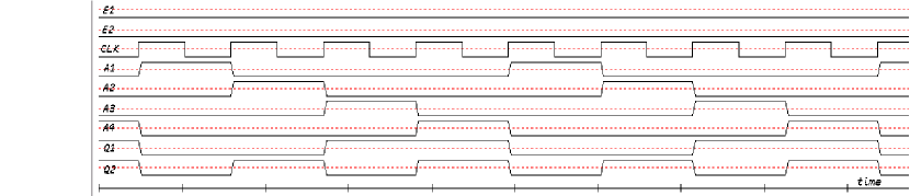
Figure 8: The wave trace of the correct program.

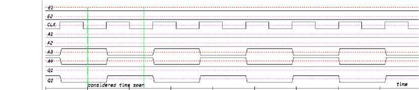
Figure 9: The wave trace of the faulty VHDL design .

Figure 10: The state-transitions for the faulty program when counting upwards.

	$t_{0}$	$t_{1}$	$t_{2}$
CLK	0	1	0
A1	0	-	0
A2	0	-	0
A3	1	-	0
A4	0	-	1

Table 1: The observations that are provided for fault localization.

After invoking the diagnosis procedure we obtained 25 single-fault diagnoses and 66 dual-fault diagnoses where each dual-fault diagnosis can be mapped back to a single bug in the source code when using the $\varphi$ function. In summary the diagnosis correspond to the statements 10, 13, 14, 15, 19, 38, 40 and 41 and include the introduced bug. The statements 10, 19, 38 and 40 correspond to a process or a conditional statements. From the remaining statements 13, 14, 15 and 41 the lines 13, 14 and 15 correspond to functional faults, i.e., wrong operators in the code. This result indicates that the new approach can localize the statement that is responsible for the misbehavior.

The new approach has been evaluated using 3 different counters. We observed that, although the quality of the computed diagnosis may vary depending on the example being used and the observations taken into account, the faulty component is always present in the computed diagnoses. Note that any of the obtained diagnoses explains the faulty behavior with respect to the given test case. However, the main obstacle towards an industrial-sized application of our approach is the computational effort that is necessary for localizing faults in larger sized real-world examples, particularly when several intermediate states are to be considered and dual- or tripe-fault diagnoses have to be computed. This problem not only arises in the context of temporal unfolding, even when considering real word sized combinatorial circuits we observed that depending on the structure of the circuit and the specific test case being used there is a large variation in the elapsed running time for computing all single-fault diagnoses.

The ISCAS’85 benchmark is a suite of combinatorial circuits used by many researchers in the field of verification, automatic test pattern generation and diagnosis. By using this suite of circuits we evaluated the running-times that have to be expected when dealing with real world problems. We have run 100 test vectors for every circuit where the test cases have been created in such a way that at least one single-fault diagnosis can be obtained for every test case. Each computation has been repeated 10 times and the minimum, the maximum, the average and the median value of the elapsed running time excluding model-setup time has been recorded. The running-times include the time for storing all the diagnoses being found. In addition, the average number of single-fault diagnoses as well as the median value of the number of single-fault diagnoses have been recorded. Table 2 outlines the results with respect to the number of single-fault diagnoses that have been obtained and Table 3 collects the elapsed running-times for computing all single-fault diagnosis. The computations were carried out on a slightly loaded Pentium 4/1.8 Ghz machine using a Visual-Works Non-Commercial Smalltalk programming environment in version 5i.4.

circuit name	median nr.	avg. nr.	gates	inputs	outputs
	(single-fault diag.)	(single-fault diag.)
C432	1	1.40	160	32	7
C499	2	2.43	202	41	32
C880	4	4.06	383	60	26
C1355	5	5.53	546	41	32
C1908	31	23.78	880	33	25
C2670	2	2.78	1193	233	140
C3540	4	5.67	1669	50	22
C5315	3	3.12	2307	178	123
C6288	306	287.02	2406	32	32
C7552	1	4.75	3512	207	108

Table 2: Average and median number of diagnosis.

circ. name	min run times	median run times	avg run times	max run times
	[ms]	[ms]	[ms]	[ms]
C432	3	14	14	41
C499	8	28	29	109
C880	$<$ 1	27	25	133
C1355	80	254	273	943
C1908	121	1397	1411	4691
C2670	$<$1	116	170	2292
C3540	377	2267	3140	17352
C5315	$<$ 1	492	520	3287
C6288	3926	122317	138910	2792591
C7552	$<$1	958	8219	75735

Table 3: Recorded running times for the different circuits.

5 Related Work, Conclusion and Further Research

Shapiro presented methods and algorithms for fault localization in logic programs Sha (83), commonly referred to as algorithmic debugging. In CFD (93) some advantages of the model-based approach over the algorithmic debugging approach are pointed out. However, as outlined in Bon (96), the model-based approach and algorithmic debugging are part of the same spectrum provided a logic program is used as the system description. Kuchcinski et al KDM (93) discusses an application of algorithmic debugging to automatic fault localization in VLSI designs and proposes a method for smooth combination of different diagnosis techniques, where the use of logic specifications and algorithmic debugging plays an essential role. The authors of KDM (93) summerize, that algorithmic debugging is similar to model-based diagnosis in that it uses a model of the correct expected behavior of the program. However, in algorithmic debugging the model is used in a probing-controlled search for faulty components rather than for generation of an exhaustive set of diagnosis hypotheses. The relationship of model-based diagnosis and algorithmic debugging is discussed in CFD (93).

In this paper we show how to create models for software debugging of hardware designs. The paper in detail discusses our value-level model for VHDL-RTL designs and shows the computation of fault locations by means of a small but practical example. Furthermore, a new model is introduced that allows for localizing faults considering the signal values during a whole time span rather than that of a certain point in time. This can be reached by unfolding our original value-based model in time and incorporating it with the semantics of process executions and event handling. Furthermore, an example indicates the principal applicability of the new approach. Moreover, the paper outlines some empirical results on the computational effort that currently is required in software debugging of real-world designs.

Besides from improving scalability, further research shall deal with model improvements by means of forward simulation, i.e., exploiting the results of a simulation to further improve our model. Recently such an approach was successfully applied in automated debugging of Java programs where the behavioral description of an if-then-else statement was considerably improved SWW (01). Another direction of current research is a detailed analysis of the outcome of our approach. Such analysis should give answers to the question whether there are kinds of faults that cannot be detected.

Further topic of future research is to incorporate the domain of verification and debugging. Verification techniques require a separate specification that, however, is often not available. If one is available though, techniques such as model checking can produce counterexamples for violated properties. Using these counterexamples to generate input for diagnosis is also part of future research.

6 Acknowledgments

The work was partially supported by the Austrian Science Fund (FWF) under project grant P15163-INF.

References

- BH (93) Lisa Burnell and Eric Horvitz. A Synthesis of Logical and Probabilistic Reasoning for Program Understanding and Debugging. In Proceedings of the International Conference on Uncertainty in Artificial Intelligence, pages 285 –291, 1993.
- Bon (96) Gregory W. Bond. Top-down consistency based diagnosis. In Proceedings of the Seventh International Workshop on Principles of Diagnosis, Val Morin, Canada, 1996.
- CFD (93) Luca Console, Gerhard Friedrich, and Daniele Theseider Dupré. Model-based diagnosis meets error diagnosis in logic programs. In Proceedings International Joint Conf. on Artificial Intelligence, pages 1494–1499, Chambery, August 1993.
- dKW (87) Johan de Kleer and Brian C. Williams. Diagnosing multiple faults. Artificial Intelligence, 32(1):97–130, 1987.
- FD (95) Yousri El Fattah and Rina Dechter. Diagnosing tree-decomposable circuits. In Proceedings International Joint Conf. on Artificial Intelligence, pages 1742 – 1748, 1995.
- FSW (99) Gerhard Friedrich, Markus Stumptner, and Franz Wotawa. Model-based diagnosis of hardware designs. Artificial Intelligence, 111(2):3–39, July 1999.
- GSW (89) Russell Greiner, Barbara A. Smith, and Ralph W. Wilkerson. A correction to the algorithm in Reiter’s theory of diagnosis. Artificial Intelligence, 41(1):79–88, 1989.
- Jac (95) Daniel Jackson. Aspect: Detecting Bugs with Abstract Dependences. ACM Transactions on Software Engineering and Methodology, 4(2):109–145, April 1995.
- KDM (93) Krzysztof Kuchcinski, Wlodzimierz Drabent, and Jan Maluszynski. Autmomatic diagnosis of VLSI digital circuits using algorithmic debugging. In P. Fritzson, editor, Proceedings of the First Workshop on Autmoated and Algorithmic Debugging, volume 749 of Lecture Notes in Computer Science, Linkoeping, Sweden, 1993.
- Kor (88) Bogdan Korel. PELAS–Program Error-Locating Assistant System. IEEE Transactions on Software Engineering, 14(9):1253–1260, 1988.
- Kup (89) Ron I. Kuper. Dependency-directed localization of software bugs. Technical Report AI-TR 1053, MIT AI Lab, May 1989.
- MSW (99) Cristinel Mateis, Markus Stumptner, and Franz Wotawa. Debugging of Java programs using a model-based approach. In Proceedings of the Tenth International Workshop on Principles of Diagnosis, Loch Awe, Scotland, 1999.
- Rei (87) Raymond Reiter. A theory of diagnosis from first principles. Artificial Intelligence, 32(1):57–95, 1987.
- Sha (83) Ehud Shapiro. Algorithmic Program Debugging. MIT Press, Cambridge, Massachusetts, 1983.
- SW (97) Markus Stumptner and Franz Wotawa. Diagnosing tree-structured systems. In Proceedings of the Eighth International Workshop on Principles of Diagnosis, Le Mont-Saint-Michel, France, 1997. Also appeared in IJCAI-97.
- SW (99) Markus Stumptner and Franz Wotawa. Debugging Functional Programs. In Proceedings International Joint Conf. on Artificial Intelligence, pages 1074–1079, Stockholm, Sweden, August 1999.
- SWW (01) Markus Stumptner, Dominik Wieland, and Franz Wotawa. Comparing two models for software debugging. In Proceedings of the Joint German/Austrian Conference on Artificial Intelligence (KI), Vienna, Austria, 2001.
- Wei (82) Mark Weiser. Programmers use slices when debugging. Communications of the ACM, 25(7):446–452, July 1982.
- Wei (84) Mark Weiser. Program slicing. IEEE Transactions on Software Engineering, 10(4):352–357, July 1984.
- Wot (00) Franz Wotawa. Debugging VHDL Designs using Model-Based Reasoning. Artificial Intelligence in Engineering, 14(4):331–351, 2000.
- Wot (02) Franz Wotawa. Debugging hardware designs using a value-based Model. Applied Intelligence, 16(1):71–92, 2002.