Rigorous design of tracers:
an experiment for constraint logic programming

Abstract

In order to design and implement tracers, one must decide what exactly to trace and how to produce this trace. On the one hand, trace designs are too often guided by implementation concerns and are not as useful as they should be. On the other hand, an interesting trace which cannot be produced efficiently, is not very useful either. In this article we propose a methodology which helps to efficiently produce accurate traces. Firstly, design a formal specification of the trace model. Secondly, derive a prototype tracer from this specification. Thirdly, analyze the produced traces. Fourthly, implement an efficient tracer. Lastly, compare the traces of the two tracers. At each step, problems can be found. In that case one has to iterate the process. We have successfully applied the proposed methodology to the design and implementation of a real tracer for constraint logic programming which is able to efficiently generate information required to build interesting graphical views of executions.

0309027171 M. Ducassé et al.AADEBUG2003: Rigorous design of tracers

IRISA/INSA de Rennes, Campus Universitaire de Beaulieu, 35042 Rennes Cedex, France

INRIA Rocquencourt, BP 105, 78153 Le Chesnay Cedex, France

1E-mail: Mireille.Ducasse@irisa.fr, {Ludovic.Langevine, Pierre.Deransart}@inria.fr 2This work is partially supported by the French RNTL project OADymPPaC, Tools for dynamic analysis of constraint logic programs, http://contraintes.inria.fr/OADymPPaC/

1 Introduction

Designing and implementing tracers is a difficult task. One must decide what exactly to trace and how to produce this trace. On the one hand, trace designs are too often guided by implementation concerns and are not as useful as they should be. On the other hand, an interesting trace which cannot be produced efficiently, is not very useful either.

Some sort of instrumentation is required to produce the trace information. This instrumentation can be done at different levels, for example the user programs can be transformed at source or compiled levels. Another possibility is to plant trace hooks in the language interpreter or emulator. All these possibilities have their advantages and drawbacks, deciding for one is not straightforward. For example, source level transformation does not require to open the compiler sources and can be efficient enough [DN00]. Instrumenting an interpreter is in general easier than working directly in the compiler and the loss in performance might be acceptable.

However, in order to have at the same time a faithful and efficient enough tracer, people often decide to instrument the language emulator or the user compiled code. In both cases, they have to dive deeply into non-obvious code. This is a tricky task, especially if the tracer developers have not been involved in the development of the compiler. At this stage, it is necessary that the trace model is stable. Instrumenting at low level requires a lot of tedious work, it is essential to know exactly what is expected before starting.

The first stage of the design, namely deciding what to trace, is, therefore, critical. However, deciding what to trace out of the blue is not obvious. It is often when people see the output of a tracer that they can tell whether the information is relevant and helpful.

To solve this apparent contradiction, we have conceived a methodology that we have successfully applied to the design and implementation of a real tracer:

1. Design a formal specification of the trace model based on an abstraction of the operational semantics of the language.

2. Derive a prototype tracer from this specification.

3. Analyze the produced traces to update or validate the trace model. This analysis can be partially automated.

4. Implement an efficient tracer.

5. Validate the efficient implementation using the prototype.

At each step, problems in the model or in implementations can be found. In that case one has to iterate the process.

The advantages of the approach are as follows. Firstly, the formal specification helps to produce a trace model which gives an accurate picture of the executions. When examining existing tracers, one too often has the feeling that they produce whatever information is easily available, hoping that the users will manage with the holes and the noise. While users often manage, mostly because they have no other choice, we claim that tracers with clean semantics are much more helpful. Secondly, in our approach the prototype is systematically derived from the trace model. It is therefore easy to produce and the resulting traces are faithful to the model. The prototype can easily produce trace samples. Thirdly, analyzing the trace samples enables people to tune the trace model. When an automated trace analyzer is used, this analysis can be systematic and thorough. Fourthly, when the tracer developers reach the stage where they have to implement a low-level tracer, they know which information is crucial and which one can be escaped. If implementation compromises have to be made, people have rational arguments to take their decisions. Lastly, comparing the actual output of the low-level implementation against the expected trace produced by the prototype is a good way to validate the quality of the implementation.

Note that the execution of the prototype tracer can afford to be slow. Indeed, it is used only at development time for qualitative reasoning, firstly to tune the trace model, then to test the implementation. Furthermore it is meant to be used on small programs only. The only requirement of these programs is that they altogether exhibit all the characteristics of the traced language. In order to test the performance of the final tracer, big programs have, of course, to be traced but with the low-level implementation not with the prototype.

The first three steps of this methodology had been applied to the retrospective design of a Prolog tracer [JDR01]. The formal specification step enabled to specify a variety of existing trace models for Prolog which were shown to be minor variants of each others. The result was a unified view of numerous models which were initially proposed without much rationale to support them. Furthermore a number of implementation issues regarding variable identifiers were detected.

More interestingly, we have used all the steps of the methodology to design from scratch a tracer for constraint logic programming over finite domains(CLP(FD) in the following). A detailed description of this tracer can be found in [LDD03]. The low-level tracer has been implemented inside the compiler of Gnu-Prolog [GP01] by somebody who did not previously know the implementation of the compiler. This experiment has been done within a project on visualization of constraint program executions, with academic and industrial partners working on different platforms. Both the formal specification of the trace model and the prototyping capabilities have enabled us to discuss with all the partners of the project and to make sure that the designed trace is indeed matching the needs of everybody. Some partners build graphical views [SA00], other provide explanations of failure for over-constrained problems [JB00]. They all work with parts of the specified trace. As the design of the trace model was not connected to a particular implementation we could design a model which is generic enough to be specialized at low cost for two different styles of constraint satisfaction (CSP [Lrg01] and CLP [Apt99]). Furthermore, some parts of the designed information, for example the list of variables and the constraint identifiers, have been proved essential for the quality of the views but they are not obvious to gather from the implementation in the emulator. Starting from the formal specification and knowing that they were absolutely needed, made them not too difficult to implement. One can conjecture that, had we started to implement straightaway the low-level implementation, these kinds of information would probably have never been provided by the tracer. Not surprisingly, in the tracers of the CLP systems, Sicstus Prolog [ASBC02] and Ilog Solver [Ilo01], in order to get the list of variables, one has to traverse a huge part of the trace. This is especially tedious to do for users.

The contribution of this article is to propose a methodology to rigorously design and validate tracer implementations. To our best knowledge, this had not been done before. This methodology has been successfully tested against the design and implementation of a real tracer.

The next sections present the methodology in more details and illustrate it with samples of the experiment done with the design, implementation and validation of a tracer for Gnu-Prolog. The explanations are meant for readers with no previous knowledge of constraint solving. Section 2 presents the trace model formalization step. Section 3 describes how to systematically derive an instrumented meta-interpreter from the formal specification. Section 4 outlines the trace analysis step. In particular, it briefly presents the connection to a trace analyzer and lists some interesting graphical views for CLP(FD). Section 5 discusses the low-level implementation of tracers. Section 6 sketches the validation of the efficient tracer against the prototype implementation.

2 Formal specification of a trace model

The first step of our methodology is to specify a trace model, namely what information about program executions should be given. In our sequential language context, a trace is a sequence of events. An event represents an interesting execution step, it can be seen as an execution breakpoint to which information is attached.

Most specifications of trace models are informal, when they exist at all. However, an informal specification is prone to misinterpretation by both developers and users. Indeed, in order to denote the events of interest, one has first to be able to denote events, and this is not easy in an informal way.

In the following, we describe two ways that have been tried to provide a formal specification of trace model, firstly an existing operational semantics has been instrumented and secondly an abstract operational semantics has been specified. We then give some details of the second experiment.

2.1 Instrumenting an existing operational semantics

Some programming languages have precise operational semantics which rigorously specify the computation steps. Hence the computation events are clearly denoted. In such a case, it is relatively easy to formally specify a trace model as shown by Jahier et al. with the Prolog tracer retro-specification [JDR01]. There were already numerous operational semantics available for Prolog. The continuation passing semantics of Nicholson and Foo [NF89] was used. Then instrumentations inside the operational semantics were specified. Only 2 rules of one line each had to be instrumented in order to get the “standard” trace of Prolog. The instrumentation itself is slightly tricky but it can be understood without ambiguity when examining a formal specification of 10 lines. The detailed description of this experiment is out of the scope of this article. Indeed, the explanations of operational semantics requires a couple of pages, understanding them requires a good knowledge of Prolog and this article is not aiming at Prolog specialists.

2.2 Specifying an abstract operational semantics

An operational semantics is not always available, for example we are not aware of any for the C language. In such a case, starting the design of the tracer by designing a complete operational semantics is certainly an overkill. An operational semantics specifies in detail the execution of a program. From an operational semantics one can derive an implementation of a compiler. In order to design a tracer, less information is usually needed than to implement a compiler. In that case, an abstract operational semantics is sufficient. The information given in an abstract operational semantics is correct but not complete. It tells tracer developers what information should be provided to users and it tells users how to interpret this trace information. In the case of CLP(FD) there was no operational semantics that we could use to specify a tracer and we designed an abstract operational semantics as a set of state transition rules. .

2.3 Informal presentation of domain reduction

Figure 1: Application of reductions to the system $\{x>y;y>z\}$.

Before we give examples of a formal specification of events we have to informally explain how variable domains are reduced. This is an essential mechanism of constraint propagation in the case of finite domains. A CLP(FD) program searches a solution for a set of variables which take values over finite domains and which must verify a set of constraints. The evolution of the domains can be viewed as a sequence of applications of reduction operators attached to the constraints. Each operator can be applied several times until the computation reaches a fix-point [FLT00]. This fix-point is the set of final domain states. An example of computation with reduction operators is shown in Figure 1. There are three variables $x$, $y$ and $z$ and two constraints, $x>y$ and $y>z$. A set of possible values is associated to each variable. This set is called the domain of the variable. The domain reduction consists in elementary steps that remove inconsistent values from those domains. At the beginning, the domain of $x$, $D_{x}$, the domain of $y$, $D_{y}$, and the domain of $z$, $D_{z}$, are all equal to $\{1,2,3\}$. This is represented by three columns of white squares. Considering the first constraint, it appears that $x$ cannot take the value “1”, because otherwise there would be no value for $y$ such that $x>y$; this inconsistent value is withdrawn from $D_{x}$. This withdrawal is marked with a black square. In the same way, the value 3 is withdrawn from the domain of $y$. Then, considering the constraint $y>z$, the sets $\{1\}$ and $\{2,3\}$ are respectively withdrawn from $D_{y}$ and $D_{z}$. Finally, using again the first constraint to propagate the previous reduction of $D_{y}$, $D_{x}$ is reduced to the singleton $\{3\}$. The fix-point is reached. The final solution is $\{x=3,y=2,z=1\}$.

2.4 Samples of formal event rules for CLP(FD)

newVariable $\displaystyle\frac{x\not\in{\cal V}}{\phantom{xx,}{\cal V}\leftarrow{\cal V}\cup\{x\},\ \ {\cal D}\leftarrow{\cal D}\cup\{(x,D_{x})\}\phantom{xx,}}~{}\{D_{x}$ : initial domain of $x\}$

newConstraint $\displaystyle\frac{\phantom{xx,}c\not\in{\cal C}\;\wedge\;\mathbf{var}(c)\subset{\cal V}\phantom{xx,}}{{\cal C}\leftarrow{\cal C}\cup\{c\}}~{}$

reject $\displaystyle\frac{\phantom{xx,}A=\{c\}\;\wedge\;unsatisfiable(c,{\cal D})\;\wedge\;R=\emptyset\phantom{xx,}}{A\leftarrow\emptyset,\ \ R\leftarrow\{c\}}~{}$

suspend $\displaystyle\frac{\phantom{xx,}A=\{c\}\;\wedge\;no\_reduction(c,{\cal D})\;\wedge\;R=\emptyset\phantom{xx,}}{A\leftarrow\emptyset,\ \ S\leftarrow S\cup\{c\}}~{}$

awake $\displaystyle\frac{\phantom{xx,,}A=\emptyset{}\;\wedge\;wake\_condition(c)\;\wedge\;R=\emptyset\phantom{xx,,}}{A\leftarrow\{c\}}~{}$

reduce $\displaystyle\frac{\;A=\{c\}\;\wedge\;x\in\mathrm{var}(c)\;\wedge\;W^{c}_{x}({\cal D})\neq\emptyset\;\wedge\;R=\emptyset\;}{D_{x}\leftarrow D_{x}-W^{c}_{x}({\cal D})}~{}\left\{\begin{array}[]{l}W^{c}_{x}({\cal D}):\hbox{ inconsistent values}\\ \hbox{ of }x\hbox{ for }c\hbox{ wrt }{\cal D}\end{array}\right\}$

Figure 2: Six rules of the abstract operational semantics defining six event types

Our abstract operational semantics is defined by a set of transition rules between observed states. An observed state is a tuple containing in particular: ${\cal C}$, the set of constraints declared until this state; ${\cal V}$, the set of finite-domain variables declared until this state;  ${\cal D}$, the set of domains of the variables declared until this state; $A$, the set of active constraints ; $S$, the set of sleeping constraints; and $R$, the set of rejected constraints which contains unsatisfiable constraints.

Figure 2 gives six examples of transition rules specifying types of events of interest. The complete trace model contains thirteen event types. Rule newVariable specifies that a new variable $x$ is introduced in $\cal V$ and that its initial domain is $D_{x}$. Rule newConstraint specifies that the solver introduces a new constraint $c$ in $\cal C$, all variables involved in $c$ are already defined. Rule reject specifies that if the active constraint ($A=\{c\}$) is unsatisfiable in the current state of the domains, it is put in the set of rejected constraints, $R$. A constraint is unsatisfiable for example when one of its variables has an empty domain. Rule suspend specifies that when an active constraint cannot reduce any domain at the moment, it is suspended in $S$. Rule awake specifies that when the set of active constraints is empty and some specific condition is fulfilled a suspended constraint can be awoken and become active . Rule reduce specifies that if the active constraint, $c$, has a variable, $x$, with inconsistent values in its domain, $W_{x}^{c}({\cal D})$, these values are withdrawn from its domain $D_{x}$.

2.5 A Trace Example

 1 newVariable   v1 =[0-268435455]
 2 newVariable   v2 =[0-268435455]
 3 newConstraint c1  fd_element([v1,[2,5,7],v2])
 4 reduce   c1   v1 =[1,2,3]   W=[0,4-268435455]
 5 reduce   c1   v2 =[2,5,7]   W=[0-1,3-4,6,8-268435455]
 6 suspend  c1
 7 newConstraint c4 x_eq_y([v2,v1])
 8 reduce   c4   v2 =[2]       W=[5,7]
 9 reduce   c4   v1 =[2]       W=[1,3]
10 suspend  c4
11 awake    c1
12 reject   c1
...

Figure 3: A portion of Trace for fd_element(I,[2,5,7],A), (A#=I ; A#=2). $a$-$b$ means from $a$ to $b$ and $a$,$b$ means $a$ and $b$

Figure 3 presents the beginning of a trace of a toy program in order to illustrate the event types described above. This program, fd_element(I, [2,5,7],A), (A#=I ; A#=2), specifies that A is a finite domain variable which is in $\{2,5,7\}$ and I is the index of the value of A in this list; moreover A is either equal to I or equal to 2. The first option is infeasible; the trace shows the events related to the failing attempt to satisfy it.

The trace can be read as follows. The first two events are related to the introduction of two variables v$1$ and v$2$, corresponding respectively toI and A. In Gnu-Prolog variables are always created with the maximum domain (from 0 to 268.435.455). Then the first constraint is created: fd_element (event #3). This constraint makes two domain reductions (events #4 and #5): the domain of the first variable (I) becomes $\{1,2,3\}$ and the domain of A becomes $\{2,5,7\}$. After these reductions, the constraint is suspended (event #6). The next constraint, A#=I, is added (event #7). Two reductions are done on variables A and I, the only possible value for A and I to be equal is 2 (events #8 and #9). After these reductions, the constraint is suspended (event #10). The first constraint is awoken (event #11). If A and I are both equal to 2, I cannot be the rank of A. Indeed, the rank of 2 is 1 and the value at rank 2 is 5. The constraint is therefore rejected (event #12). The execution continues and find the solution A=2 and I=1. This requires 20 other events not shown here

2.6 Discussion

Our semantics does not specify how the rules are applied but what events are of interest and what information is available at each event. As already mentioned, it helps tracer developers to design the tracer and it helps tracer users to interpret the produced traces.

For example, rule reject tells the implementor that whenever the solver finds an unsatisfiable constraint, the tracer should be called with this constraint. The same rule tells users that when they see a reject event in a trace, the corresponding constraint has become unsatisfiable and there was previously no rejected constraint.

Similarly, rule reduce tells the implementor that, when the solver processes a reduction, the tracer should be called with information about the related constraint, the related variable and the new domain $D_{x}$. The same rule tells users that when they see a reduce event in a trace, the reduction has been achieved on one of the variables of the specified constraint, that there were inconsistent values to remove from this variable and that there was previously no rejected constraint. The trace also gives the inconsistent values that have been withdrawn. Incidentally, the rule also specifies that the constraint that prompted the reduction is still the active one ($A$ is not modified).

Note that the upper part of the rules are not shown in actual traces, this is implicit information. In most tracers, users have to guess it. In our system, it is explicit, at least in the formal specification.

3 Implementation of a prototype tracer

A formal specification of trace model is helpful to formally reason about a trace. However, it actually specifies many traces for many kinds of solvers. It is sometime too arid to decide whether possible traces can be of any help to users. With that respect, it is better to have samples of execution traces checked by “guinea pig users”. Producing samples by hand is very tedious. It becomes quickly untractable since the trace model evolves according to the remarks of the guinea pigs! New samples have therefore to be produced until a trace model is validated by users. It is, thus, welcome to have a tracer as quickly as possible. However, a low-level implementation is not suited before the trace model has been validated by users. As already mentioned in the introduction, we propose to use a prototype tracer in order to break this deadlock.

3.1 Derivation of a prototype tracer from the CLP(FD) trace model

In our CLP(FD) experiment, we derive a CLP(FD) interpreter coded in Prolog that we instrument with trace hooks. Figure 4 contains the translation of reject and reduce rules of Figure 2. Each rule is encoded by a predicate with the same name as the rule.

[1]1 reject(St0, St) :- St0 = ([C], S, Q, T, [], D), get_varC(C, VarC), member(X, VarC), get_domain(X, D, []), St = ( [], S, Q, T, [C], D), trace(reject, C, St0, _, _, _).

reduce(St0, St, ModOut) :- St0 = ([C], S, Q, T, [], D0), get_varC(C, VarC), member(X, VarC), reduction(C, D0, X, Wx), update_domain(X, Wx, D0, D, ModOut), St = ([C], S, Q, T, [], D), trace(reduce, C, St0, X, Wx, ModOut).

Figure 4: Translation into Prolog of the reject and reduce rules of Figure 2

Before paraphrasing the code for one rule, we give the meaning of all the (simple) predicates that are used and not defined: get_varC(C, V) takes as input a constraint C and outputs a list of the constraint variables that appear in C; member(X, L) is a standard Prolog predicate which checks whether X is an element of the list L; get_domain(X, D, Dx) takes a constraint variable X and a domain state D, and outputs the domain of $X$ (Dx); note that in Prolog = denotes a unification; trace(Port, C, St0, Att1, Att2, Att3) takes as input the different event attributes; it calls the trace analysis system which can, for example, print a trace line; reduction(C, D, X, Wx) takes as input a constraint C, a domain state D, a constraint variable X, and outputs the values to withdraw from the domain of X; it fails if Wx $=\emptyset$ (no reduction can be done); 
update_domain(X, Wx, D0, D, Mod) takes as input a constraint variable X, a value set Wx (to withdraw), and a domain state D0; it outputs the state domain D such that Dx=D0 - Wx, and the list of modification types $X_{mod_{1}}$, …, $X_{mod_{n}}$, where $mod_{i}\in\{min,max,ground,any,empty\}$. These modifications characterize the Wx value withdrawal.

All the predicates implementing transition rules take as input a solver state St0 and output a new solver state St. St0 and St respectively denote the state of the solver before and after the application of a rule. Predicate reject(St0, St) implements the reject rule. That rule needs to fulfill 3 conditions to be allowed to be applied: firstly, there is a constraint C in the active constraint set, secondly the set of rejected constraints is empty, and thirdly there exists a variable attached to the C constraint whose domain is empty. This last condition implies the $unsatisfiable(c,{\cal D})$ predicate of Figure 2. The first two conditions are checked line 2. The third condition is checked lines 3 to 5 using Prolog backtracking. The execution of this predicate will backtrack to member(X, VarC) until either there is no more variables in VarC or one of them has an empty domain. After the application of the rule the set of active constraints is empty and the set of rejected constraints contains $C$ (line 6). The tracer is called with the relevant information (line 7). Note the use of Prolog anonymous variables for arguments 3 to 6. This means that the values are meaningless. The other rules are implemented in the same way.

The rules are integrated into the underlying Prolog system in the usual meta-interpretation way of Prolog. This is not detailed in this article. An introduction to meta-interpreters in Prolog can be found in [SS94].

3.2 Discussion

We have been able to systematically deduce the Prolog code from the specification. Even if the production of the prototype tracer was not automatic, it has been sufficiently systematic so that the modifications of the trace model could be immediately integrated. Furthermore, it has always been easy to convince ourselves that the produced prototypes indeed implemented the expected trace model.

The produced prototype tracer was rather slow, but as already mentioned in the introduction, efficiency is not an issue at this stage. The idea is to validate the trace model, the tracer designers use the prototype on well chosen and small programs.

The formal specification is very useful, but if time and resources are short, and if the prototype tracer is very simple and easy to implement, it can be considered to start the design of the tracer with the prototype. One will miss the formal support for verification but at least there will be some means to think about the trace design.

In our experiments, we have used the meta-interpretation capabilities of logic programming to build prototype tracers. Even in languages with no meta-programming capabilities, there are always some means to easily produce prototypes. For example a source-level instrumentation of a subset of the language is generally possible. Not all the features and libraries of a language need to be instrumented in the prototype. If the syntax of the language is specified by a grammar, then the instrumentation can be implemented inside this grammar, for example with an attributed grammar language such as Yacc.

4 Trace analysis

Once a first trace model is designed and a prototype tracer exists, it is important to play with actual traces. As soon as the traces are longer than what can be printed on a page it becomes very tedious to analyze them by hand. Even toy programs can produce traces of thousands of events whose systematic display would be inefficient and irrelevant. Therefore, we believe that the validation can be much more rigorous and powerful if it is automated. In our approach we connect the prototype tracer with an automated trace analyzer à la Opium [Duc99b]. The first advantage is that many long traces can be systematically tested. A second advantage is that abstract and graphical views can be automatically built [Duc99a, Jah00]. In the case of CLP we have built a number of graphical views which helped us select from the potential interesting trace information the ones that were really important and the ones that were not so crucial. It should be noted that, applying the methodology, the trace model that we designed varied quite a lot between the first design [LDDJ01] and the current one [LDD03].

In the remaining of this section we first present the generic trace querying facility. We then sketch one example of interesting graphical view of CLP(FD) executions which has been built with the trace analyzer.

4.1 Analysis of the produced trace

In our trace analysis scheme, users can formulate queries in order to investigate an execution trace. The queries are formulated in the Prolog language extended by two primitives: fget/1 and
get_attr/2. fget/1 searches for a specific event forward in the execution trace, get_attr/2 retrieves data about the current event.

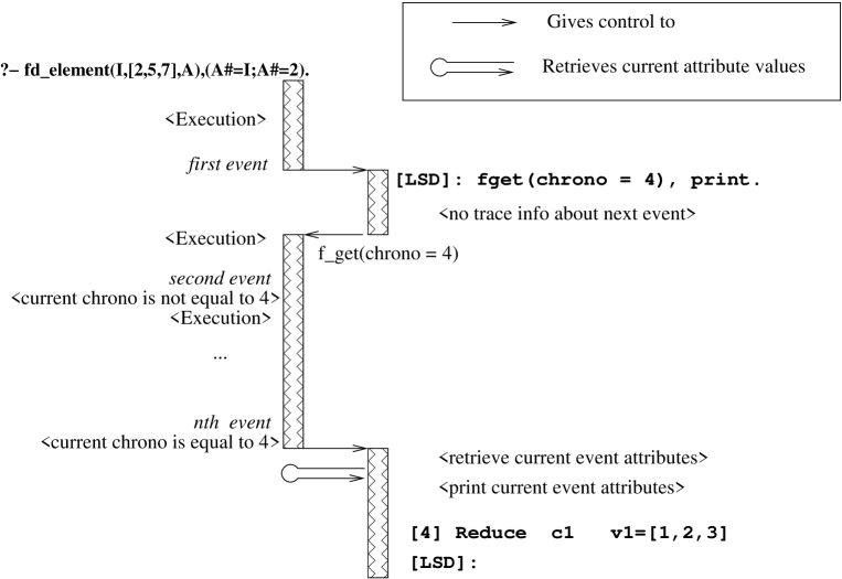
Figure 5: Illustration of the processing of a filtering query

Events are searched for as the traced program is executed. There are two execution processes, one for the traced execution, and one for the trace analysis (called LSD in the following). Figure 5 illustrates how the fget/1 primitive works. Let us assume that the programmer wants to query the execution trace of the program given in Figure 3. When the execution reaches the first event, it notifies LSD which prompts the programmer for a trace query. The programmer enters a goal in order to search forward until an event with chronological number equal to 4 is found (fget([chrono=4])). This event should then be displayed (print). At that moment, LSD can only get information about the current event. It therefore returns control to the traced execution. When the traced execution reaches the next event, it locally checks whether the current chrono is equal to 4. As the current chrono is not the requested one, the traced execution is resumed until the next event is reached. The chrono is again locally checked. Forward moves and checking are done in turn until the first event whose chrono is 4. LSD is notified and proceeds. The current event attributes are retrieved by the print command which displays the related information. The execution of the trace query is completed. The programmer is then prompted for another one.

The scheme previously described is a good compromise between efficiency and expressive power. On the one hand, the search for events is done in the traced process, and can be very efficient. On the other hand, as the whole power of Prolog is available in the analyzer process, sophisticated debugging programs can be written.

[1]1 :- fget([port = reduce, chrono>3]), get_attr([var, withdrawn], [X, Wx]).

:- setval(nb_reject, 0), fget(in(port, [reject, solution])), ( get_attr(port, reject) -> incval(nb_reject), fail ; true ), getval(nb_reject, NbFailures), writeln(NbFailures).

Figure 6: Two examples of trace queries

Two examples of composed queries are given in Figure 6. The first query asks to go to the first event whose port is reduce with a chronological number (chrono) greater than 3. The reduced variable and the withdrawn domain are then retrieved and stored in the variables X and Wx On the trace given in Figure 3, the query would find the fourth event and return X=v1 and Wx=[0,4-268435455].

The second query of Figure 6 is an example of sophisticated query which could be integrated into an analysis program. It counts the number of failures encountered before the first solution and prints it. First, the counter is initialized (line 4). The fget primitive is used to find the next event whose port is either reject or solution (line 5). Then the actual port is retrieved with get_attr (line 6). If it is reject, then the counter is incremented (line 7) and a failure is forced (line 8). If it is not a reject, it means that it is a solution; in that case the loop is stopped by simply executing true (line 9). In the case where the execution is made to fail, it will backtrack to the fget which will find the next event whose port is either reject or solution (line 5). If the execution does no longer contain such events, the overall query will simply fail. In the case where the loop terminates on a solution the value of the counter is retrieved (line 11) and printed (line 12).

4.2 A CLP(FD) visualization of variable updates

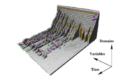
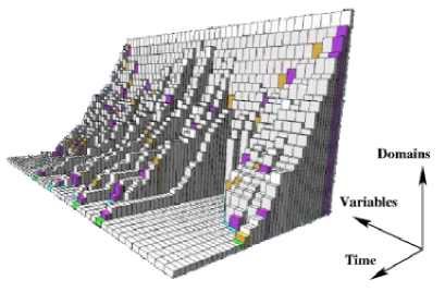
Figure 7: Comparing two search procedures for the 40-queens problem with VRML views computed by trace analysis.

One of our experiments is the generation of a 3D variable update view. The evolution of the domains of the variables during the computation is displayed in three dimensions. It gives a tool à la TRIFID [CH00]. The trace analyzer computes domain size each time a constraint is added to the store or rejected, as well as when a solution is found. The details of reduce events allow us to assign color to each kind of domain update (for example minimum or maximum value removed or domain emptied) as made by Simonis and Aggoun in the Cosytec Search-Tree Visualizer [SA00]. The trace analysis is implemented in about 125 lines of Prolog and generates an intermediate file. A program implemented in 240 lines of C converts this file into the VRML format.

Figure 7 shows the resolution of the 40-queens problem with two different enumeration strategies. There are three axes: variables, domain size and time. The first strategy is a first-fail selection of the enumerated variable and the first value tried is the minimum of its domain. The second strategy is also a first-fail strategy but variable list is sorted with the middle variable first and the middle of domain is preferred to its minimum. The two graphical views allow users to compare the efficiency of these two strategies by manipulating the 3D-model. With the first strategy, domain sizes on one side of the chess-board quickly decrease, and the domain size on the other side oscillate at length. With the second strategy, domain sizes decrease more regularly and more symmetrically, the solution is found faster. In fact, the second strategy, which consists in positioning the queens starting from the center of the chess-board, benefits more from the symmetrical nature of the problem.

4.3 Discussion

The list of all the variables attached to the problem is a relevant information because graphical views such as the 3D-model display all the domains at a glance whereas the solver handles only a small subset of variables at a time. The above experiments made clear that the tracer must be able, if requested, to provide the whole state at each event, namely the domains and the constraints of the problem. Furthermore, the list of variables involved in a given constraint is not straightforward to get from the implementation. However, this kind of information is also crucial to build some graphical views which are helpful to users. Even if producing these types of information requires some implementation efforts and may have a cost in terms of performance, it is worth producing them. This was not possible to decide by just looking at the formal semantics.

5 Efficient implementation

When the trace designer knows what in the expected trace model is important for which debugging functions. The actual implementation can start. The events of interest have to be located in the compiler or compiled code. It is also necessary to specify how to get the information related to each event. At this stage, the tracer implementors can decide that a piece of information is too tricky or too costly to produce. This happens all the time in tracers produced without this methodology. The essential difference here is that the tracer implementors know what is kept or not and why. This is important for users. For example, if a particular graphical view requires some information which cannot be generated in a particular implementation, users will know straightforwardly and will not discover it the hard way.

5.1 The Gnu-Prolog tracer implementation

Encoding a trace model that is not derived from the actual implementation of the solver is a delicate task. The correspondence between a formalized event and the code of the solver is not obvious: some events can be almost simultaneous, or a single event can be performed in several points of the code. For example, the trace model provides a unified view of the domain reduction with the reduce rule whereas there are several places to instrument in the code. Domain reduction is a crucial point in a constraint solver and the corresponding code is highly optimized. In Gnu-Prolog, there are four different cases for the domain reduction, depending on the way the values to withdraw have been computed. The tracer handles each case with its peculiarities in order to get a single reduction event. Whatever domain reduction routine is used, the trace event will be a reduce with standard attributes.

Another issue is the ability to proceed through the whole sets of constraints and variables, as well as to allocate them unique identifiers. The solver only handles pointers on data structures. During the execution, a given pointer can be used for several constraints and variables. Moreover, at a given moment, the solver focuses on a small subset of entities. Therefore the tracer has to maintain its own data structures to reference all the pointers the solver handles. When the solver creates a new variable or a new constraint, the tracer references the pointer on this new entity in a specific table. This table associates to this pointer a new integer identifier and some debugging data that can be useful in the sequel. When the solver deletes some constraints and variables, the corresponding entries are removed from the tracer table. This table can be used to search for an identifier knowing the pointer on an entity or to search for a pointer knowing the identifier of an entity. Both of these uses are made in logarithmic time. Another possible use is retrieving the list of all the variables or the list of all the constraints.

The methodology has led to a trace model that is far from the implementation of Gnu-Prolog. The trace has needed the instrumentation of critical points in the solver. Nevertheless, the implementation has been possible and the final model has a clear semantics that is easy to understand for a constraint programmer. Moreover, the resulting tracer is efficient: the time overhead while executing a program without any trace output is between 5 and 30 percents (less than 10% in most of our benchmarks). While producing a very detailed trace (with almost all the attributes the model provides), the time ratio against an untraced execution is between 3 and 7.4. These performances are comparable to other debuggers known to be efficient enough, for example the Mercury tracer of Somogyi and Henderson [SH99] or the ML tracer of Tolmach and Appel [TA95].

It is worth noticing that the tracer has been implemented in such a way that only the part of the trace which is required by a specific analysis is constructed: users pay only for what they need.

5.2 Discussion

Two other tracers exist for constraint programming. The first one is the trace mechanism of the Ilog Solver platform. Ilog Solver is a C++ library for constraint solving. Some virtual trace functions are called at some specific points of the solver. By default, those functions do nothing. The developer can redefine them to produce his own trace. The parameters of the trace functions are the attributes of the corresponding trace events. Taking the critical example of domain reduction, we see that trace events are guided by the implementation: there are two events by special case Ilog Solver handles: an event before and an event after. Their attributes depend on the case that is active. At the opposite, our model and implementation provide a single unified event with all the data at a glance.

The second existing tracer is an experimental tracer for Sicstus Prolog. Its trace model is dedicated to Sicstus implementation. The tracer is based on a complete storage of the trace and postmortem investigation. When a specific data on an event is asked for, the tracer has to traverse the trace backwards until the data is found or is able to be recomputed. Most of our trace model could be produced this way but it is not realistic for real-life executions.

6 Validation

Another important problem when building a tracer is to validate the result. In particular, it is important to be sure that the produced trace is indeed the expected one. As opposed to the prototype, the efficient implementation has no obvious relation to the formal specification.

Our methodology proposes to further take benefits of the prototype implementation in order to compare the traces produced by the actual tracer with the trace produced by the prototype. This comparison is not expected to be a bijection in the general case. Indeed, some events may not be implemented (see the discussion above), some information may not be available. In addition, the actual tracer may also produce larger traces for example for the parts of the language and libraries that were not taken into account in the prototype. As a consequence, at present, the comparison between the two types of traces has to be done by hand.

6.1 Validation of the Gnu-Prolog tracer implementation

Prototype trace: [1]1 newVariable v1 =[1,2,3] newVariable v2 =[2,5,7]

Gnu-Prolog trace: [1]3 newVariable v1 =[0-268435455] newVariable v2 =[0-268435455] newConstraint c1 fd_element([v1,[2,5,7],v2]) reduce c1 v1 =[1,2,3] W=[0,4-268435455] reduce c1 v2 =[2,5,7] W=[0-1,3-4,6,8-268435455] suspend c1

Figure 8: Portions of traces, with some attributes produced by the prototype tracer and Gnu-Prolog tracer for the introduction of new variables

For our experiment we compared the traces of the executions of some small programs produced by the prototype tracer and the Gnu-prolog tracer. Figure 8 shows portions of trace related to the introduction of a new variable. In the prototype tracer, the variables are directly introduced with their specified domain. In the Gnu-Prolog solver, every time a new variable is introduced, its domain initially contains all the possible values and the following execution steps use the regular reduction mechanism to reduce the domain to the one which was declared. In our example, the two events of lines 1 and 2 produced by the prototype tracer correspond to the events of lines 3 to 8 produced by the Gnu-Prolog tracer. These events appear in Figure 3 and have already been explained in section 2.5.

6.2 Discussion

Besides the identification of some minor implementation problems, this analysis led us to refine the constraint identifiers to take into account the fact that in Gnu-Prolog some built-in constraints are split into several simpler constraints. The need for this refinement could probably have been detected by other means, the systematic comparison of the two types of traces, however, was a good support to find problems in the low-level implementation, and this quite early in the life time of the software.

7 Conclusion

In this article we have presented a methodology to rigorously design and implement tracers in 5 steps: 1) design a formal specification of the trace model, 2) derive a prototype tracer, 3) analyze the produced traces, 4) implement an efficient tracer, 5) compare the traces produced by the efficient implementation and the prototype.

The methodology has been used within the context of logic programming where there is a strong background on semantics. We, however, believe that the state transition approach can be applied to specify formal trace models for other programming paradigms.

Even if we advocate to follow the complete methodology, some of the steps can be useful without the others. For example, even without a formal specification, starting with an easy to build and understand prototype tracer is already a major improvement over starting directly by the implementation of a low-level tracer.

We have shown how this methodology has been used to design and implement a real tracer for CLP(FD) which is able to efficiently generate information required to build interesting graphical views of executions. The trace model has been designed following mainly user’s concerns whereas usual tracers are designed following mainly implementation concerns. The resulting tracer has performances comparable to efficient tracers, therefore the methodology improves the quality of the produced trace, and does not prevent efficiency.

References

- [Apt99] K. Apt. The essence of constraint propagation. Theoretical Computer Science, 221(1-2):179–210, 1999.
- [ASBC02] M. Agren, T. Szeredi, N. Beldiceanu, and M. Carlsson. Tracing and explaining execution of CLP(FD) programs. In A. Tessier, editor, Proc. of the Workshop on Logic Proramming Environmement. CoRR repository cs.SE/0207047, July 2002.
- [CH00] M. Carro and M. Hermenegildo. The VIFID/TRIFID tool. In Deransart et al. [DHM00], chapter 10.
- [DHM00] P. Deransart, M. Hermenegildo, and J. Maluszynski, editors. Analysis and visualization tools for constraint programming, volume 1870 of Lecture Notes in Computer Science. Springer-Verlag, 2000.
- [DN00] M. Ducassé and J. Noyé. Tracing Prolog programs by source instrumentation is efficient enough. Journal of Logic Programming, 43(2):157–172, May 2000.
- [Duc99a] M. Ducassé. Abstract views of Prolog executions with Opium. In P. Brna, B. du Boulay, and H. Pain, editors, Learning to Build and Comprehend Complex Information Structures: Prolog as a Case Study, Cognitive Science and Technology, chapter 10, pages 223–243. Ablex, 1999.
- [Duc99b] M. Ducassé. Opium: An extendable trace analyser for Prolog. The Journal of Logic programming, 39:177–223, 1999. Special issue on Synthesis, Transformation and Analysis of Logic Programs, A. Bossi and Y. Deville (eds), Also Rapport Technique INRIA 3257.
- [FLT00] G. Ferrand, W. Lesaint, and A. Tessier. Value withdrawal explanation in CSP. In M. Ducassé, editor, AADEBUG’00 (Fourth International Workshop on Automated Debugging), pages 188–201, 2000. The COmputer Research Repository (CORR) cs.SE/0012005.
- [GP01] GNU-Prolog. A clp(fd) system based on Standard Prolog (ISO) developed by D. Diaz, 2001. http://gprolog.sourceforge.net/ Distributed under the GNU license.
- [Ilo01] Ilog. Solver 5.1 reference manual, 2001.
- [Jah00] E. Jahier. Collecting graphical abstract views of Mercury program executions. In M. Ducassé, editor, Proceedings of the International Workshop on Automated Debugging (AADEBUG2000), Munich, August 2000. Refereed proceedings, the COmputer Research Repository (CORR) cs.SE/0010038.
- [JB00] N. Jussien and V. Barichard. The palm system: explanation-based constraint programming. In Proceedings of TRICS: Techniques foR Implementing Constraint programming Systems, a post-conference workshop of CP 2000, pages 118–133, Singapore, September 2000.
- [JDR01] E. Jahier, M. Ducassé, and O. Ridoux. Specifying Prolog trace models with a continuation semantics. In K.-K. Lau, editor, Logic Based Program Synthesis and Transformation. Springer-Verlag, Lecture Notes in Computer Science 2042, 2001.
- [LDD03] L. Langevine, M. Ducassé, and P. Deransart. A propagation tracer for Gnu-Prolog: from formal definition to efficient implementation. In C. Palamidessi, editor, Proceedings of the 19th Int. Conf. in Logic Programming. Springer-Verlag, Lecture Notes in Computer Science, December 2003.
- [LDDJ01] L. Langevine, P. Deransart, M. Ducassé, and E. Jahier. Tracing executions of clp(fd) programs: a trace model and an experimental validation environment. Rapport de Recherche RR 4342, INRIA, Novembre 2001.
- [Lrg01] F. Laburthe and the OCRE research group. CHOCO, a Constraint Programming kernel for solving combinatorial optimization problems, September 2001. Available at http://www.choco-constraints.net.
- [NF89] T. Nicholson and N. Foo. A denotational semantics for Prolog. ACM Transactions on Programming Languages and Systems, 11(4):650–665, 1989.
- [SA00] H. Simonis and A. Aggoun. Search-tree visualisation. In Deransart et al. [DHM00], chapter 7.
- [SH99] Z. Somogyi and F. Henderson. The implementation technology of the Mercury debugger. In Proceedings of the Tenth Workshop on Logic Programming Environments, volume 30(4). Elevier, Electronic Notes in Theoretical Computer Science, 1999. http://www.elsevier.nl/cas/tree/store/tcs/free/entcs/store/tcs30/cover.sub.sht.
- [SS94] L. Sterling and E. Shapiro. The Art of Prolog, second edition. MIT Press, Cambridge, Massachusetts, 1994. ISBN 0-262-19338-8.
- [TA95] A. Tolmach and A.W. Appel. A debugger for Standard ML. Journal of Functional Programming, 5(2):155–200, April 1995.