A Combinatorial Characterization of Higher-Dimensional Orthogonal Packing

Abstract

Higher-dimensional orthogonal packing problems have a wide range of practical applications, including packing, cutting, and scheduling. Previous efforts for exact algorithms have been unable to avoid structural problems that appear for instances in two- or higher-dimensional space. We present a new approach for modeling packings, using a graph-theoretical characterization of feasible packings. Our characterization allows it to deal with classes of packings that share a certain combinatorial structure, instead of having to consider one packing at a time. In addition, we can make use of elegant algorithmic properties of certain classes of graphs. This allows our characterization to be the basis for a successful branch-and-bound framework.

This is the first in a series of papers describing new approaches to higher-dimensional packing.

Keywords: higher-dimensional packing and cutting, orthogonal structures, geometric optimization, discrete structures, interval graphs, comparability graphs, cocomparability graphs, branch-and-bound, exact algorithms

AMS classification: 90C28, 68R99

1 Introduction

The problem of cutting a rectangle into smaller rectangular pieces of given sizes is known as the two–dimensional cutting stock problem. It arises in many industries, where steel, glass, wood, or textile materials are cut, but it also occurs in less obvious contexts, such as machine scheduling or optimizing the layout of advertisements in newspapers. The three-dimensional problem is important for practical applications such as container loading or scheduling with partitionable resources. It can be thought of as packing boxes into a container. When arranging these boxes in a container $C$, we have to preserve the orientations of the boxes; this constraint usually arises from considerations for stability in packings (“this side up”), from asymmetric texture of material in cutting-stock problems, or from different types of coordinates in scheduling problems. In the context of technical computer science, ?) consider an application of three-dimensional packing to dynamic reconfiguration of hardware; one of the axes corresponds to time, the two others to different spatial dimensions.

We refer to the generalized problem in $d\geq 2$ dimensions as the $d$-dimensional orthogonal knapsack problem (OKP-$d$). Being a generalization of the bin packing problem (BPP), the OKP-$d$ is ${\cal NP}$-complete in the strict sense – see ?). The vast majority of work done in this field refers to a restricted problem, where only so–called guillotine patterns are permitted. This constraint arises from certain industrial cutting applications: guillotine patterns are those packings that can be generated by applying a sequence of edge-to-edge cuts; see ?) and ?). The recursive structure of these patterns makes this variant much easier to solve than general or non–guillotine problems.

Relatively few authors have dealt with the exact solution of non–guillotine problems. All of them focus on the problem in two dimensions. ?) gave a characterization of non–guillotine patterns using network flows but derived no algorithm. ?) proposed an exact algorithm for the case that all boxes have equal size. ?) extended an approach for guillotine problems to cover a certain type of non–guillotine patterns. So far, only two exact algorithms have been proposed and tested for the general case of knapsack problems. ?) and ?) have given different 0–1 integer programming formulations for this problem. Even for small problem instances, they have to consider very large 0–1 programs, because the number of variables depends on the size of the container that is to be packed. The largest instance that was solved in either article has 9 out of 22 boxes packed into a 30 $\times$ 30 container. (See the “OR-Library” by ?) for a number of test instances.) After an initial reduction phase, ?) gets a 0-1 program with over 8000 variables and more than 800 constraints; the program by Hadjiconstantinou and Christofides still contains more than 1400 0–1 variables and over 5000 constraints. From Lagrangian relaxations, they derive upper bounds for a branch–and–bound algorithm that are improved using subgradient optimization. The process of traversing the search tree corresponds to the iterative generation of an optimal packing.

We should note that more recently, two papers on the related problem of two- and three-dimensional bin packing have been presented: ?) consider the two-dimensional case, while ?) deal with three-dimensional bin packing. We discuss aspects of those papers in [Fekete and Schepers 1997c], when considering bounds for higher-dimensional packing problems. Even more recently, ?) gave a mixed integer programming formulation for three-dimensional packing problems, similar to the one anticipated by the second author in his thesis [Schepers 1997]. Padberg expressed the hope that using a number of techniques from branch-and-cut will be useful; however, he did not provide any practical results to support this hope.

In this paper we describe a different approach to characterizing feasible packings and constructing optimal solutions. We use a graph-theoretic characterization of the relative position of the boxes in a feasible packing. This allows a much more efficient way to construct an optimal solution for a problem instance: combined with good heuristics for dismissing infeasible subsets of boxes, we develop a two-level tree search. This exact algorithm has been implemented; it outperforms previous methods by a wide margin.

The rest of this paper is organized as follows: after a formal problem description in Section 2, we introduce the novel concept of packing classes in Section 3 and show that it suffices to deal with the existence of feasible packings. In Section 4, we describe algorithmically useful properties of packing classes, and highlight algorithmic difficulties in Section 5. In [Fekete and Schepers 1997d], we give a detailed description of how packing classes can be combined with other algorithmic ideas for obtaining powerful exact algorithms for orthogonal packing problems.

2 Preliminaries

Why are two- and higher-dimensional packing problems harder to solve than their one-dimensional counterparts?

In order to decide whether another item can be packed into a partially filled container, in the one-dimensional case, we only need to know the total size of the items that have already been placed. When dealing with a two- or higher-dimensional problem, we also need to know the arrangement of boxes, i.e., their packing. Thus, the performance of an algorithm for higher-dimensional packing hinges on the use of an appropriate representation of packings.

A main difficulty is highlighted by the following easy observation: In general, the feasible space for packing further objects into a container is not convex. This means that we cannot simply formulate a higher-dimensional orthogonal packing problem as a straightforward integer linear program. Nevertheless, ?) and ?) have used such a formulation, where the free space is controlled with the help of a large number of 0,1-variables, describing a partition of the feasible space into convex pieces. They only consider the two-dimensional case. These formulations lead to very large 0,1-programs, even for packing problems of moderate size. It seems hopeless to try this approach for three-dimensional instances of relevant size.

We present an alternative approach to these 0,1-formulations. Our new way of modeling packings is based on a graph-theoretic characterization of packings. It can be used for any number of dimensions and leads to the central term of packing class, which describes a whole family of combinatorially equivalent feasible packings. The implementation of the resulting algorithms is described in detail in [Fekete and Schepers 1997d].

We start by introducing some basic notation and definitions.

2.1 Problem Description and Notation

In the following, we consider a set of items that need to be packed into a container. We concentrate on $d$-dimensional boxes, and the items are also called boxes.

The input data for a $d$-dimensional orthogonal packing problem is a finite set of boxes $V$, and a (vector-valued) size function $w:V\rightarrow{{\rm{\sf I}\kern-4.19998ptQ}^{\scriptstyle+}_{\scriptstyle 0}}^{d}$ that describes the size of each box in any dimension $x_{1},\ldots,x_{n}$. For the orthogonal knapsack problem (OKP), we also have a value function $v:V\rightarrow{{\rm{\sf I}\kern-4.19998ptQ}^{\scriptstyle+}}$ that describes the objective function value for each box.

The size of the container is given by a vector $W\in{{\rm{\sf I}\kern-4.19998ptQ}^{+}}^{d}$. Without loss of generality, we assume that each individual box fits into the container, i. e., $w(b)\leq W$ holds for each box.

For the volumes of boxes and container we use the following notation. If $b\in V$, and $w$ is a size function defined on $V$, then

$${\mbox{\it vol}}_{w}(b):=\prod_{i=1}^{d}w_{i}(b)$$

denotes the volume of box $b$ with respect to $w$. Similarly, the volume of the container is denoted by

$${\mbox{\it vol}}_{W}:=\prod_{i=1}^{d}W_{i}.$$

If $S$ is a finite set and $f$ a real-valued function on $S$, then we use the abbreviation

$$f(S):=\sum_{x\in S}f(x).$$

Finally, we use the notation $\{v,w\}$ for an edge in an undirected graph; we write $(v,w)$ when referring to a directed edge. For a given set of vertices $S\subseteq V$ in a graph $G=(V,E)$, an induced subgraph is given by $G[S]=(S,E[S])$, with $E[S]$ being the set of edges in $G$ that connect vertices in $S$. For a vertex $v\in V$ in a directed graph $G=(V,E)$, $\delta^{-}(v)$ denotes the indegree of $v$. More graph-theoretic terms will be introduced when needed. In all cases, see the book by ?) for more background.

2.2 Orthogonal Packings

We consider arrangements of boxes that satisfy the following constraints:

1. Orthogonality: Each face of a box is parallel to a face of the container.

2. Closedness: No box may exceed the boundaries of the container.

3. Disjointness: No two boxes may overlap.

4. Fixed Orientations: The boxes must not be rotated.

In the following, we imply these conditions when “packing boxes into a container”, “considering a set of boxes that fits into a container”, and speak of packings.

In order to formalize the notion of a packing, we introduce a Cartesian coordinate system with axes parallel to the edges of the container. The origin is one corner of the container, which is fully contained in the positive orthant. Thus, a packing is a function that maps each box to the coordinates of the one of its corners that is closest to the origin.

Definition 1 (Packing)

 
Given a set of boxes $V$, a size function $w$, and a container size $W$.

A function $p:V\rightarrow{{\rm{\sf I}\kern-4.19998ptQ}^{\scriptstyle+}_{\scriptstyle 0}}^{d}$ is called a packing of $(V,w,W)$, iff

$$\forall b\in V: p(b)+w(b)\leq W$$ (1)

$$\forall b,c\in V,b\neq c,\exists i\in\{1,\dots,d\}: I^{p}_{i}(b)\cap I^{p}_{i}(c)=\emptyset.$$ (2)

Here, $I^{p}_{i}(b)$ denotes the interval $[\,p_{i}(b),p_{i}(b)+w_{i}(b)\,)$, for a box $b\in V$, and a direction $i\in\{1,\dots,d\}$.

Condition (1) implies closedness, while (2) implies disjointness of the boxes. Because components of the size function are fixed, we pack with fixed orientations.

Remark 1

The condition “p is a packing for $(V,w,W)$” can be expressed by linear constraints. For this purpose, condition (2) has to be replaced by

$$\forall b,c\in V,b\neq c\bigvee_{i=1}^{d}\,p_{i}(b)+w_{i}(b)\leq p_{i}(c)\,\vee\,p_{i}(c)+w_{i}(c)\leq p_{i}(b).$$

In ?), p. 12f., it is described how the disjunction can be transformed into $2d+1$ linear inequalities by using $2d$ additional 0,1-variables. The resulting mixed integer programs seem to be beyond practical size. Our own experience with a mixed integer approach has been far from promising, see ?); it remains to be seen whether the more recent revival by ?) will lead to any computational results.

2.3 Objective Functions

Depending on the objective function, we distinguish three types of orthogonal packing problems:

Definition 2 (Optimization Problems)

• The Strip Packing Problem (SPP) asks for the minimal height $W_{d}$ of a container that can hold all boxes, where the size in the other $d-1$ dimensions $W_{1},\ldots,W_{d-1}$ are fixed.

• For the Orthogonal Bin Packing Problem (OBPP), we have to determine the minimal number of identical containers that are required to pack all the boxes.

• In the Orthogonal Knapsack Problem (OKP), each box has an objective value. A container has to be packed such that the total value of the packed boxes is maximized.

This classification follows the scheme introduced by ?). (He introduces a fourth class called Pallet Loading, where all boxes have identical size and value $1$; this is a special case of the knapsack problem.) To clarify the dimension of a problem, we may speak of OKP-$2$, OKP-$3$, OKP-$d$, etc.

Problems SPP and OBPP are closely related. For $d\in{\rm I\kern-1.79993ptN}$, an OBPP-$d$ instance can be transformed into a special type of SPP-$(d+1)$ instance, by assigning the same $x_{d+1}$-size to all boxes. This is of some importance for deriving relaxations and lower bounds.

For all orthogonal packing problems we have to satisfy the constraint that a given set of boxes fits into the container. This subproblem is of crucial importance for our approach.

Definition 3 (Orthogonal Packing Problem  (OPP-$d$))

For a set of boxes $V$, a size function $w$, and the container size $W$, is there a packing for $(V,w,W)$?

Clearly, the OPP is the decision problem for the above optimization problems.

3 Problem formulation and mathematical approach

3.1 Modeling the Problem

In the following, we describe a new way of modeling feasible packings. The basic idea is to use the combinatorial information induced by relative box positions. For this purpose, we consider projections along the different coordinate axes; overlap in these projections defines an interval graph for each coordinate. Using properties of interval graphs and additional conditions, we can tackle two fundamental problems of exact enumeration algorithms:

1. How can we prove in reasonable time that a particular subset of boxes is infeasible for packing?

2. How do we avoid treating equivalent cases more than once?

3.2 Packing classes

Instead of dealing with single packings we handle classes of packings that share a certain combinatorial structure. This structure arises from the way different boxes in a packing can “see” each other orthogonal to one of the coordinate axes. (So-called box visibility graphs have been considered as means for representing graphs, e.g., see the references in ?).) We will see that transitive orientations of certain classes of graphs correspond to possible packings if and only if specific additional conditions are satisfied. This allows us to make use of a number of powerful theorems [Ghouilà-Houri 1962, Gilmore and Hoffmann 1964, Golumbic 1980, Korte and Möhring 1989] to perform pruning of our branch-and-bound tree.

For a $d$-dimensional packing, consider the projections of the boxes onto the $d$ coordinate axes $x_{i}$. Each of these projections induces a graph $G_{i}=(V,E_{i})$:

$$\{b,c\}\in E_{i}\Leftrightarrow I_{i}^{p}(b)\cap I_{i}^{p}(c)\neq\emptyset.$$

In other words, two boxes are adjacent in $G_{i}$, if and only if their $x_{i}$ projections overlap. (See Figure 1 for a two-dimensional example.) By definition, the $G_{i}$ are interval graphs, thus they have algorithmically useful properties that are described in Section 4.

Figure 1: A two-dimensional packing and the interval graphs $G_{1}$, $G_{2}$ induced by the axis-parallel projections.

A set of boxes $S\subseteq V$ is called $x_{i}$–feasible, if $\sum_{b\in S}w_{i}(b)\leq W_{i}$, i.e., if the boxes in $S$ can be lined up along the $x_{i}$–axis without exceeding the $x_{i}$–width of the container. Finally, it follows from the disjointness condition (2) that no two boxes may overlap in all coordinate projections. Thus, we get the following necessary conditions:

Observation 1

For any feasible packing, the graphs $G_{i}=(V,E_{i}),i=1,\ldots,d$ have the following properties:

$$P1: G_{i}:=(V,E_{i})$$ Each is an interval graph.

$$P2: \mbox{Each stable set }S\mbox{ of }G_{i}\mbox{ is $x_{i}$--feasible}.$$

$$P3: \bigcap_{i=1}^{d}E_{i}=\emptyset.$$

The main result of this paper is the converse: These three conditions are also sufficient.

A family of $E=(E_{1},\ldots,E_{d})$ of edges sets for a vertex set $V$ representing a set of boxes is called a packing class for $(V,w)$, if and only if it satisfies the conditions $P1$, $P2$, $P3$. For any given $G_{i}=(V,E_{i})$, we denote by $\overline{G_{i}}$ the complement graph $(V,\overline{E_{i}})$ for $G_{i}$. See Figure 2. If $G_{i}$ arises from a packing, any edge in $\overline{G_{i}}$ corresponds to two boxes with non-overlapping $x_{i}$-projection, hence we can think of $\overline{G_{i}}$ as the comparability graph of the boxes in direction $x_{i}$: Two boxes are comparable (and hence there is an edge in $\overline{G_{i}}$), if their $x_{i}$-projections do not overlap, and one projection lies strictly to the left of the other projection.

Next we consider directed graphs arising from some of these undirected graphs, indicating the partial order of the $x_{i}$-projections. A directed graph $D=(V,A)$ is called a transitive orientation of a graph $G=(V,E)$, iff there is a bijection ${\cal O}:E\rightarrow A$ with the property

$$(a,b)\in A\wedge(b,c)\in A\Rightarrow(a,c)\in A.$$

Note that this implies that the undirected edge $\{a,c\}$ must also be contained in $E$. For more background on transitive orientations, see the book by ?).

For any packing class $E$, we consider transitive orientations $F_{i}$ of the comparability graph $\overline{G_{i}}$, and call $F=(F_{1},\dots,F_{d})$ a transitive orientation of the packing class $E$. In the following, we show that for any transitive orientation $F$ of a packing class, there is a packing. For this purpose, define a mapping $p_{i}^{F}:V\rightarrow{{\rm I\!R}^{+}_{0}}^{d}$ by

$$p^{F}_{i}(v):=\max\{p^{F}_{i}(u)+w_{i}(u)|(u,v)\in F_{i}\}$$ (3)

for $v\in V,\,i\in\{1,\dots,d\}$.

3.3 Sufficiency of Packing Classes

Without loss of generality, it is sufficient to consider packings that are generalized “bottom-left” justified, such that any lower bounding coordinate of a box is at zero or at the upper bounding coordinate of another box (without requiring the two boxes to touch). More formally, we say that a packing is gapless, if

$$\quad\forall i\in\{1,\dots,d\}\ \forall v\in V:\quad p_{i}(v)=0\quad\vee\quad\exists u\in V:\,p_{i}(v)=p_{i}(u)+w_{i}(u).$$

In the following, we show that the above three conditions on the graphs forming a packing class are not only necessary for the existence of a packing, but they are also sufficient, even for the subclass of gapless packings. This implies that a packing class is not just a set of graphs, but can also be interpreted as a whole equivalence class of feasible packings.

Lemma 1

Any packing class $E$ represents a feasible packing. More precisely, for a transitive orientation $F$ of $E$, the function $p^{F}:V\rightarrow{{\rm I\!R}^{+}_{0}}^{d}$ describes a gapless packing.

Proof:  Consider a packing class $E$. As each $G_{i}=(V,E_{i})$ is an interval graph, the complement $\overline{G_{i}}$ is a comparability graph, hence it has a transitive orientation $F_{i}$. Let $F=(F_{1},\ldots,F_{d})$ be any such set of transitive orientations. As defined above, this induces a mapping $p^{F}$. We place all boxes $v$ at the positions given by $p^{F}(v)$. To show that $p^{F}$ is a packing, we have to show that

1. All boxes are within the boundaries of the container.

2. No two boxes overlap.

To establish 1., we show that at any stage there must be a set of boxes that determines the overall $x_{i}$-width of the partial packing, so by $P2$, the partial packing must fit in all directions. For this purpose, let $v\in V,i\in\{1,\ldots,d\}$. By construction of $p^{F}$, the acyclic digraph $(V,F_{i})$ contains a directed path $(v^{(0)},\ldots,v^{(r)})$ with $\delta^{-}(v^{(0)})=0$ and $v^{(r)}=v$, such that

$$p^{F}_{i}(v)=\sum_{k=0}^{r-1}w_{i}(v^{(k)}).$$

Because $F_{i}$ is transitive, $S:=\{v^{(0)},\ldots,v^{(r)}\}$ induces a clique in $\overline{G_{i}}$, implying that $S$ is a stable set in $G_{i}$. Hence by condition $P2$,

$$p_{i}^{F}(v)+w_{i}(v)=\sum_{k=0}^{r}w_{i}(v^{(k)})\leq W_{i},\mbox{ implying 1.}$$

To see 2., consider $u,v\in V$, $u\neq v$. By $P3$, there is an $i\in\{1,\dots,d\}$ with the (undirected) edge $\{u,v\}\notin E_{i}$, hence $\{u,v\}\in\overline{E_{i}}$. Because $F_{i}$ is an orientation of $\overline{E_{i}}$, either $(u,v)\in F_{i}$ or $(v,u)\in F_{i}$. By construction of $p^{F}$, we get

$$p^{F}_{i}(v)\geq p^{F}_{i}(u)+w_{i}(u)\quad\lor\quad p^{F}_{i}(u)\geq p^{F}_{i}(v)+w_{i}(v).$$

In both cases, $u$ and $v$ can be separated by an $x_{i}$-orthogonal hyperplane. Hence, the boxes $u$ and $v$ are disjoint and $p^{F}$ describes a packing. By construction of $p^{F}$, the packing is gapless. $\quad\Box$

From Observation 1 and Lemma 1, the main theorem of this paper follows:

Theorem 1

A set of $d$-dimensional boxes $V$ can be packed into a container, iff there is a packing class $E$ for $(V,w)$, i.e., a set of $d$ graphs $G_{1},\ldots,G_{d}$ with the properties P1, P2, P3.

The proof of Lemma 1 shows constructively that any orientation of a packing class corresponds to a packing; basically, an orientation $(v_{1},v_{2})$ of an edge $\{v_{1},v_{2}\}\in E_{i}$ means that $v_{1}$ can “see” $v_{2}$ along the positive $x_{i}$-axis. To illustrate the structure, we give the following example:

Example 1

Consider the OPP-$2$ $P=(V,w)$, defined by

$$V:=\{b_{1},b_{2},b_{3},b_{4},b_{5}\}$$

$$w(b_{1}):=\left(4,1\right),\quad w(b_{2}):=\left(5,1\right),\quad w(b_{3}):=\left(1,3\right),$$

$$w(b_{4}):=\left(2,2\right),\quad w(b_{5}):=\left(1,2\right),\quad W:=\left(5,5\right).$$

and the packing class $E$ for $P$ as shown in Figure 1. (Note that box $i$ is darker than box $j$ whenever $i<j$.)

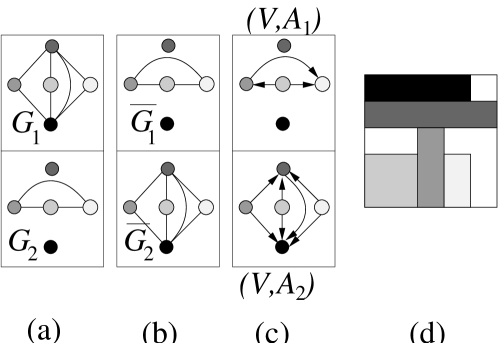
Figure 2: Constructing a packing for a two-dimensional packing class $E$: (a) A pair of interval graphs. (b) The corresponding complement, i.e., comparability graphs. (c) Transitive orientations of the comparability graphs. (d) A packing built from the transitive orientations. It is feasible by properties $P2$ and $P3$.

The complements of the component graphs $E_{1}$ and $E_{2}$ from the example in Figure 2 each have six transitive orientations. Hence there are 36 transitive orientations of $E$. Figure 3 shows the corresponding packings, constructed by virtue of (3).

Figure 3: All feasible packings of the packing class $E$ from Figure 2 (a).

Remark 2

Independent from our work, an approach with some similarity to our packing classes can be found in an unpublished report by ?). In that report, two-dimensional packings are described as pairs of complements of partial orders. However, Jerrum does not observe that there is a purely combinatorial characterization that allows it to map graphs to packings, as described in our Lemma 1. The latter is the main result of this paper.

We conclude this section by a graph-theoretic formulation of a useful geometric property.

If a set of boxes $S$ has a total sum of $x_{i}$-widths exceeding $k$ times the $x_{i}$-width of the container, then any feasible packing must have an $x_{i}$–orthogonal cut that intersects at least $k+1$ boxes. Using the terminology of packing classes, we get an algorithmically useful formulation of this condition:

Theorem 2

Let $E$ be a packing class for $(V,w)$, $i\in\{1,\dots,d\}$, $G_{i}:=(V,E_{i})$ and $S\subseteq V$. Then $G_{i}[S]$ contains a clique of size $\left\lceil\frac{\sum_{s\in S}w_{i}(s)}{W_{i}}\right\rceil$.

Proof:  As an interval graph, $G_{i}$ is perfect. Thus, the induced subgraph $G_{i}[S]$ has maximum clique size $\omega:=\omega(G_{i}[S])$ equal to the chromatic number $\chi(G_{i}[S])$. Hence, $S$ can be partitioned into $\omega$ disjoint stable sets: $S=\dot{\cup}_{k=1}^{\omega}S_{k}$. All stable sets from $G_{i}[S]$ are also stable in $G_{i}$. Then $P2$ implies for all $k\in\{1,\dots,\omega\}$ that $w_{i}(S_{k})\leq 1$. Altogether, we get

$$w_{i}(S)=w_{i}\left(\bigcup_{k=1}^{\omega}S_{k}\right)=\sum_{k=1}^{\omega}w_{d}(S_{k})\leq\omega.$$

Because $\omega$ is integer, the claim follows. $\quad\Box$

A more elaborate discussion on bounds for higher-dimensional packing and their applications can be found in ?).

4 Algorithmic Implications

When trying to solve a packing problem to optimality, a crucial step is deciding the orthogonal packing problem (OPP) whether a particular set of boxes can be packed in a feasible way. In a practical context, one will typically use three different tools:

(1) In order to see whether there is a fast positive answer we can try to find a packing by means of a heuristic.

(2) A fast way to get a negative answer is described in ?), where we discuss lower bounds for packing problems.

However, for hard instances, both of these approaches will fail to provide an answer, meaning that a third tool has to be applied:

(3) If all else fails, we need to resort to an appropriate enumeration method to solve the OPP.

In this section, we describe how packing classes can be used to provide (3) if both of the easy approaches fail. (Because the OPP is NP-hard in the strong sense (?)), it is reasonable to use enumerative methods.)

As we saw above, the existence of a packing is equivalent to the existence of a packing class. Furthermore, we have shown that a feasible packing can be constructed from a packing class in time that is linear in the number of edges. This allows us to search for a packing class, instead of a packing. As we describe in the following, the advantage of this approach lies not only in exploiting the symmetries arising from different transitive orientations of the same packing class, but also in the fact that the structural properties of packing classes give rise to very efficient rules for identifying irrelevant portions of the search tree.

Some of the technical implementation details of the enumeration scheme are rather involved; they are described in [Fekete and Schepers 1997d]. Here we give an overview over the underlying mathematical ideas.

4.1 Building Packing Classes

When trying to build a packing class $E_{1},\ldots,E_{d}$ for a set of boxes, we use a branch-and-bound approach. The algorithm branches by fixing any edge $\{b,c\}\in E_{i}$ or by excluding it via $\{b,c\}\notin E_{i}$. The set of edges that are “positively fixed” to be in some $E_{i}$ is called $E_{+}$, while the set of “negatively fixed” edges that are excluded are called $E_{-}$. Fixing an edge to be in $E_{+}$ is called augmenting $E_{+}$, while excluding it means augmenting $E_{-}$. When referring to a particular $E_{i}$, the respective sets of included and excluded edges are denoted by $E_{+,i}$ and $E_{-,i}$.

The branching has two possible objectives:

1. Augment $E_{+}$ until it is a packing class.

2. Prove that no augmentation of $E_{+}$ to a packing class is possible, as it would have to use “excluded ” edges from $E_{-}$.

In the first case, our tree search has been successful. In the second case, the search on the current subtree may be terminated, because the search space is empty. Otherwise, we have to continue branching until one of the two objectives is reached.

In the following we show how graph-theoretic properties can be exploited to help with these objectives.

4.2 Excluded Induced Subgraphs

Following the idea described in the previous paragraph, we need three components for our enumeration scheme:

(1) A test “Is the current set of fixed edges $E_{+}$ a packing class?”

(2) A sufficient criterion that $E_{+}$ has no feasible augmentation.

(3) A construction method for feasible augmentations.

All three of these components can be reduced to identifying or avoiding particular induced subgraphs.

First of all, it is easy to determine all edges that are excluded by condition $P3$. By performing these augmentations of $E_{-}$ immediately, we can guarantee that $P3$ is satisfied. Thus we can assume that $P3$ is satisfied, and will remain satisfied by further augmentations.

$P2$ explicitly excludes certain induced subgraphs: $i$-infeasible stable sets, i. e., $i$-infeasible cliques in the complement of each component graph.

In order to formulate $P1$ in terms of excluded induced subgraphs, we use the following powerful Propositions 1 and 2 – the reader is referred to the book by ?). In this context, we use a couple of technical terms:

Definition 4 (Chords, Cocomparability Graphs)

For a cycle $C:=[b_{0},\dots,b_{k-1},b_{k}=b_{0}]$ of length $k$, the edges $b_{i}b_{j},i,j\in\{0,\dots,k-1\}$ with $(|i-j|\mbox{ mod }k)>1$ are called chords; the chords $b_{i}b_{j},i,j\in\{0,\dots,k-1\}$ with $(|i-j|\mbox{ mod }k)=2$ are called $2$-chords of $C$. A cycle is ($2$-) chordless, iff it does not have any ($2$-) chords.

A graph is called triangulated, if it does not contain any chordless cycle of length $k\geq 4$.

A graph $G=(V,E)$ is a cocomparability graph, if the complement graph $G=(V,\overline{E})$ is a comparability graph.

In a graph $G=(V,E)$, $\{v_{1},v_{2},v_{3}\}\subseteq V$ is called an asteroidal triple, if any two of the vertices can be connected by a path that contains no vertex adjacent to the third vertex.

Proposition 1 (Gilmore and Hoffman 1964)

A cocomparability graph is an interval graph, iff it does not contain the chordless cycle $C_{4}$ of length 4 as an induced subgraph.

Proposition 2 (Ghouilà-Houri 1962, Gilmore and Hoffman 1964)

A graph is a comparability graph, iff it does not contain a $2$-chordless cycle of odd length.

In the proof of Theorem 3, we will make use of yet another characterization of interval graphs.

Proposition 3 (Lekkerkerker and Boland 1962)

A graph is an interval graph, iff it is a triangulated graph that does not contain any asteroidal triple.

Thus, $E_{+}$ is a packing class, if for all $i\in\{1,\dots,d\}$ the following holds (recall that $P3$ is assumed to be satisfied):

1. $(V,E_{+,i})$ does not contain a $C_{4}$ as an induced subgraph.

2. $(V,{E_{-,i}})$ does not contain an odd $2$-chordless cycle.

3. $(V,{{E}_{-,i}})$ does not contain an $i$-infeasible clique.

For illustration, we provide the following example:

Example 2

See Figure 4. Consider $V=\{v_{1},v_{2},v_{3},v_{4}\}$ and suppose that at some stage, we have

$$E_{+,i}=\{\{v_{1},v_{2}\},\{v_{3},v_{4}\},\{v_{4},v_{1}\}\}$$

and

$$E_{-,i}=\{\{v_{2},v_{4}\},\{v_{1},v_{3}\}\}.$$

This leaves the decision for the edge $\{v_{2},v_{3}\}$. Adding $\{v_{2},v_{3}\}$ to $E_{+,i}$ would create an induced $C_{4}$ in $(V,E_{+,i})$; by Theorem 1, this is not admissible, forcing $\{v_{2},v_{3}\}$ to be in $E_{-,i}$.

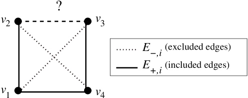
Figure 4: Making use of Proposition 1: The edge $\{v_{2},v_{3}\}$ must be added to $E_{-,i}$ to avoid an induced $C_{4}$.

In [Fekete and Schepers 1997d], we describe the technical details how these properties can be implemented for achieving a fast algorithm. The computational results described there show that the overall code outperforms previous approaches by a wide margin.

5 A Complexity Result

Tackling the OPP by building a packing class resolves some of the difficulties, but of course there is little hope of solving the problem in polynomial time by any method. We conclude this paper by pointing out the exact nature of the remaining difficulty.

Because properties $P1$ and $P3$ appear easy to deal with, it is natural to suspect that this difficulty lies in property $P2$. Thus, it seems reasonable to hope for an efficient method that preserves properties $P1$ and $P3$ when augmenting a “partial packing class”: Given a $d$-tuple of edge sets that satisfies $P3$, can it be augmented such that properties $P1$ and $P3$ are satisfied? (Note that $P2$ would be inherited to all augmentations, because any stable set after an augmentation must have been a stable set before.) A polynomial algorithm for this task would reduce the computational difficulty of solving the OPP by means of enumeration.

Formally, we have the following problem:

Definition 5 (Disjoint $d$-Interval Graph Completion Problem (DIGCP-$d$)

GIVEN:	graphs ${\cal G}_{1}=(V,{\cal E}_{+,1}),\dots,{\cal G}_{d}=(V,{\cal E}_{+,d})$ with $\bigcap_{i=1}^{d}{\cal E}_{+,i}=\emptyset$.
QUESTION:	For $i\in\{1,\dots,d\}$, is there a superset $E_{i}$ for each ${\cal E}_{+,i}$, such that
	$\bigcap_{i=1}^{d}E_{i}=\emptyset$, and the graphs $G_{1}=(V,E_{1}),\dots,G_{d}=(V,E_{d})$ are interval
	graphs?

In the dissertation of the second author [Schepers 1997] it is shown that the existence of a polynomial algorithm for this problem is highly unlikely: The OPP remains NP-hard, even if we have a $d$-tuple of edge sets that satisfies $P2$ and $P3$. This indicates that it is indeed $P1$ that makes life difficult.

Theorem 3

For $d\geq 2$, the Disjoint $d$-Interval Graph Completion Problem is NP-complete.

Proof:  Recognizing interval graphs can be done in linear time [Korte and Möhring 1989], so the problem is in NP.

For showing that the problem is NP-hard, we give a reduction of 3SAT. In the following, all notation is consistent with [Garey and Johnson 1979].

Constructing a DIGCP-2 instance from a 3SAT instance:

Consider a Boolean expression $\Phi$ in conjunctive normal form with variables $u_{1},\dots,u_{n}$ and clauses $c_{1},\dots,c_{m}$. The following DIGCP-2 instance can be constructed in polynomial time:

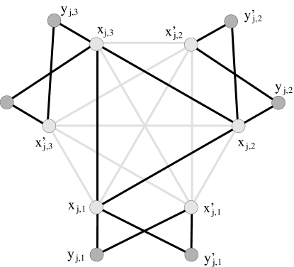
Figure 5: The edges used for representing clauses.

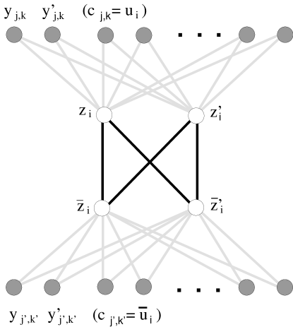
Figure 6: The edges used for representing variables.

1. For each clause $c_{j}$ define six interior vertices $x_{j,k},x_{j,k}^{\prime},\,k\in\{1,\dots,3\}$ and six exterior vertices $y_{j,k},y_{j,k}^{\prime},\,k\in\{1,\dots,3,\}$. Connect these vertices according to Figure 5. The black edges form the set $C_{j}^{(1)}$, and the gray edges form the set $C_{j}^{(2)}$. Thus we have

   $$C_{j}^{(1)} = \{\{x_{j,1}x_{j,2}\},\{x_{j,1}x_{j,3}\},\{x_{j,2}x_{j,3}\}\}\cup\bigcup_{k=1}^{3}\{x_{j,k}y_{j,k},x_{j,k}y_{j,k}^{\prime},x_{j,k}^{\prime}y_{j,k},x_{j,k}^{\prime}y_{j,k}^{\prime}\},$$

   $$C_{j}^{(2)} = \{x_{j,1}^{\prime}x_{j,2}^{\prime},x_{j,1}^{\prime}x_{j,3}^{\prime},x_{j,2}^{\prime}x_{j,3}^{\prime}\}\cup\bigcup_{k=1}^{3}\bigcup_{\scriptstyle l=1\atop\scriptstyle l\neq k}^{3}\{x_{j,k}x_{j,l}^{\prime}\}.$$

2. For each variable $u_{i}$ define the four vertices $z_{i},z_{i}^{\prime},\bar{z}_{i},\bar{z}_{i}^{\prime}$. If $u_{i}$ is the $k$th literal in clause $c_{j}$, then $z_{i},z_{i}^{\prime}$ are connected with the exterior vertices $y_{j,k}$ and $y^{\prime}_{j,k}$ of $c_{j}$. If $\bar{u}_{i}$ is the $k$th literal of clause $c_{j}$, $\bar{z}_{i},\bar{z}_{i}^{\prime}$ are connected with $y_{j,k}$ and $y^{\prime}_{j,k}$. Thus, we get the two edge sets

   $$U_{i}^{(2)}:=\{z_{i}y_{j,k},z_{i}^{\prime}y_{j,k},z_{i}y_{j,k}^{\prime},z_{i}^{\prime}y_{j,k}^{\prime}|\quad\mbox{ $u_{i}$ is the $k$-th literal of $c_{j}$}\}$$

   and

   $$\bar{U}_{i}^{(2)}=\{\bar{z}_{i}y_{j,k},\bar{z}_{i}^{\prime}y_{j,k},\bar{z}_{i}y_{j,k}^{\prime},\bar{z}_{i}^{\prime}y_{j,k}^{\prime}\quad|\quad\mbox{ $\bar{u}_{i}$ is the $k$-th literal of $c_{j}$}\}$$

   These edges are shown gray in Figure 6. The black edges form the set

   $$U_{i}^{(1)}=\{z_{i}\bar{z}_{i},z_{i}\bar{z}_{i}^{\prime},z_{i}^{\prime}\bar{z}_{i},z_{i}^{\prime}\bar{z}_{i}^{\prime}\}.$$

Now the DIGCP-$2$ instance $I$ is given by

$$V := \bigcup_{j=1}^{m}\bigcup_{k=1}^{3}\left\{x_{j,k},x_{j,k}^{\prime},y_{j,k},y_{j,k}^{\prime}\right\}\,\cup\,\bigcup_{i=1}^{n}\left\{z_{i},z_{i}^{\prime},\bar{z}_{i},\bar{z}_{i}^{\prime}\right\}$$

$${\cal E}_{+,1} := \bigcup_{j=1}^{m}C_{j}^{(1)}\,\cup\,\bigcup_{i=1}^{n}U_{i}^{(1)}$$

$${\cal E}_{+,2} := \bigcup_{j=1}^{m}C_{j}^{(2)}\,\cup\,\bigcup_{i=1}^{n}U_{i}^{(2)}\,\cup\,\bigcup_{i=1}^{n}\bar{U}_{i}^{(2)}.$$

Constructing a solution for 3SAT from a solution of DIGCP-2:

Let now $(E_{1},E_{2})$ be a solution of $I$. For $i\in\{1,\dots,n\}$ let

$$u_{i}:=\left\{\begin{array}[]{ll}\mbox{\tt TRUE},&z_{i}z_{i}^{\prime}\notin E_{1}\\ \mbox{\tt FALSE},&z_{i}z_{i}^{\prime}\in E_{1}\end{array}\right.$$

In order to show that this assignment of variables satisfies $\Phi$, we will repeatedly use Proposition 3. In particular, the proposition implies that an interval graph cannot contain an asteroidal triple or a $C_{4}$ as an induced subgraph.

If $u_{i}=\mbox{\tt TRUE}$, hence $z_{i},z_{i}^{\prime}\notin E_{1}$, then $\bar{z}_{i}\bar{z}_{i}^{\prime}\in E_{1}$ must hold; Otherwise the edge set $\{z_{i},\bar{z}_{i},z_{i}^{\prime},\bar{z}_{i}^{\prime}\}$ would induce a $C_{4}$ in $(V,E_{1})$.

Let $c_{j}$ be a clause in $\Phi$. In Figure 5 consider the subgraph induced in ${\cal E}_{+,2}$ by the interior vertices of $c_{j}$ that has the edge set $C_{j}^{(2)}$. We note the following.

1. No vertex of the path $(x_{j,1},x_{j,3}^{\prime},x_{j,2})$ is adjacent to $x_{j,3}$ by an edge in $C_{j}^{(2)}$

2. No vertex of the path $(x_{j,1},x_{j,2}^{\prime},x_{j,3})$ is adjacent to $x_{j,2}$ by an edge in $C_{j}^{(2)}$

3. No vertex of the path $(x_{j,2},x_{j,1}^{\prime},x_{j,1})$ is adjacent to $x_{j,1}$ by an edge in $C_{j}^{(2)}$

Thus, the vertices $x_{j,1}$, $x_{j,2}$, $x_{j,3}$ form an asteroidal triple, unless one or several edges prevent this by introducing adjacencies. More precisely, $E_{2}$ must contain at least one of the edges $x_{j,1}x_{j,1}^{\prime}$, $x_{j,2}x_{j,2}^{\prime}$, $x_{j,3}x_{j,3}^{\prime}$ in addition to $C_{j}^{(2)}$, because all other edges that could destroy the asteroidal triple are in ${\cal E}_{+,1}$.

Without loss of generality let $x_{j,1}x_{j,1}^{\prime}\in E_{2}$ and hence $x_{j,1}x_{j,1}^{\prime}\notin E_{1}$. In order to prevent the four vertices $\{x_{j,1},y_{j,1},x_{j,1}^{\prime},y_{j,1}^{\prime}\}$ from inducing a $C_{4}$ in $(V,E_{1})$, $y_{j,1}y_{j,1}^{\prime}\in E_{1}$ must hold. Using the same argument on $E_{2}$, $y_{j,1}y_{j,1}^{\prime}\notin E_{2}$ implies that the edge $z_{i}z_{i}^{\prime}$ (or $\bar{z}_{i}\bar{z}_{i}^{\prime}$, resp.) belonging to the first literal $u_{i}$ (or $\bar{u}_{i}$, resp.) must be in $E_{2}$, hence not in $E_{1}$. Corresponding to our chosen truth assignment, we get $u_{i}=\mbox{\tt TRUE}$ (or $u_{i}=\mbox{\tt FALSE}$, resp.) Therefore, clause $c_{j}$ is satisfied for any $j$, and hence $\Phi$.

Constructing a solution for DIGCP-2 from a solution of 3SAT.

Consider a truth assignment of the $u_{i}$ that satisfies $\Phi$. Without loss of generality, let the first literal in each clause be TRUE, and let $i\in\{1,\dots,n\}$.

If $u_{i}={\tt TRUE}$, let

$$\hat{U_{i}}^{(1)} := U_{i}^{(1)}\cup\{\bar{z}_{i}\bar{z}_{i}^{\prime}\},$$

$$\hat{U_{i}}^{(2)} := U_{i}^{(2)}\cup\{z_{i}z_{i}^{\prime}\},$$

$$\hat{\overline{U_{i}}}^{(2)} := \bar{U_{i}}^{(2)}\cup\mbox{$E_{A}$}\mbox{ with }A:=\{y_{j,k},y_{j,k}^{\prime}|\mbox{ $\bar{u}_{i}$ is the $k$-th literal of $c_{j}$}\}.$$

If $u_{i}={\tt FALSE}$, let

$$\hat{U_{i}}^{(1)} := U_{i}^{(1)}\cup\{z_{i}z_{i}^{\prime}\},$$

$$\hat{U_{i}}^{(2)} := U_{i}^{(2)}\cup\{\bar{z}_{i}\bar{z}_{i}^{\prime}\},$$

$$\hat{\overline{U_{i}}}^{(2)} := \bar{U_{i}}^{(2)}\cup\mbox{$E_{B}$}\mbox{ with }B:=\{y_{j,k},y_{j,k}^{\prime}|\mbox{ $u_{i}$ is the $k$-th literal of $c_{j}$}\}.$$

It is easy to see that the corresponding subgraphs are interval graphs:

For $j\in\{1,\dots,m\}$, let

$$\hat{C_{j}}^{(1)} := C_{j}^{(1)}\cup\{y_{j,1}y_{j,1}^{\prime},x_{j,2}x_{j,2}^{\prime},x_{j,3}x_{j,3}^{\prime}\}\,\cup\,\{y_{j,1},y_{j,1}^{\prime}\}\times\{x_{j,2},x_{j,2}^{\prime},y_{j,2},y_{j,2}^{\prime}\}$$

$$\hat{C_{j}}^{(2)} := C_{j}^{(2)}\cup\{(x_{j,1}x_{j,1}^{\prime})\}$$

The representations shown in Figures 7 and 8 show that $(V,\hat{C_{j}}^{(1)})$ and $(V,\hat{C_{j}}^{(2)})$ are also interval graphs.

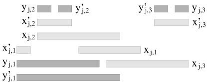
Figure 7: Representing $(V,\hat{C_{j}}^{(1)})$ by intervals.

Figure 8: Representing $(V,\hat{C_{j}}^{(2)})$ by intervals.

Let now

$$E_{1} := \bigcup_{i=1}^{n}\hat{U_{i}}^{(1)}\cup\bigcup_{j=1}^{m}\hat{C_{j}}^{(1)},$$

$$E_{2} := \bigcup_{i=1}^{n}\hat{U_{i}}^{(2)}\cup\bigcup_{i=1}^{n}\hat{\overline{U_{i}}}^{(2)}\cup\bigcup_{j=1}^{m}\hat{C_{j}}^{(1)}.$$

$(V,E_{1})$ and $(V,E_{2})$ are interval graphs, because all their connected components are. ${\cal E}_{+,1}\subseteq E_{1}$ and ${\cal E}_{+,2}\subseteq E_{2}$ follows immediately from the construction.

For $j\in\{1,\dots,m\}$, let $u_{i}$ be the first literal from clause $c_{j}$. By assumption, this literal has the value TRUE, implying that the edge $y_{j,1}y_{j,1}^{\prime}$ does not belong to $\hat{U}_{i}$ or $\hat{\overline{U}}_{i}$, resp. Therefore, $\hat{C}_{i}$ is disjoint from these edge sets. This excludes the only possible overlap of $E_{1}$ and $E_{2}$, implying $E_{1}\cap E_{2}=\emptyset$. Therefore, $(E_{1},E_{2})$ is a solution of the DIGCP-2 instance $I$. $\quad\Box$

6 Conclusions

In this paper, we have introduced a new way of characterizing higher-dimensional packings of a set of boxes into a container. Using graph-theoretic structures, this characterization has a number of nice algorithmic properties. We describe in [Fekete and Schepers 1997d] how these properties can be used for implementing an exact algorithm that is able to solve two- and three-dimensional packing problems of relevant size. Our implementation makes extensive use of new classes of lower bounds for higher-dimensional packing problem; the mathematical background is described in ?). The overall algorithm appears to have convincing performance; this should make the mathematical structures and properties described in this paper interesting to a wide audience.

Our graph-theoretic characterization has also turned out to be useful in practical applications in which there are additional spatial constraints in some of the dimensions. See ?) for an application arising from dynamic reconfiguration of hardware. Making further use of order-theoretic structures, we have been able to extend this approach to handle order constraints. Details are described in ?).

References

- Arenales and Morábito 1995 Arenales, M. N. and R. Morábito (1995). An AND/OR graph approach to the solution of two–dimensional non–guillotine cutting problems. Eur. J. Oper. Res. 84, 599–617.
- Beasley 1985 Beasley, J. E. (1985). An exact two–dimensional non–guillotine cutting tree search procedure. Oper. Res. 33, 49–64.
- Beasley 1990 Beasley, J. E. (1990). OR-library: distributing test problems by electronic mail. J. Oper. Res. Soc. 41, 1069–1072.
- Biró and Boros 1984 Biró, M. and E. Boros (1984). Network flows and non–guillotine cutting patterns. Eur. J. Oper. Res. 16, 217–221.
- Christofides and Whitlock 1977 Christofides, N. and C. Whitlock (1977). An algorithm for two–dimensional cutting problems. Oper. Res. 25, 31–44.
- Dowsland 1987 Dowsland, K. A. (1987). An exact algorithm for the pallet loading problem. Eur. J. Oper. Res. 31, 78–84.
- Fekete, Köhler, and Teich 2001 Fekete, S. P., E. Köhler, and J. Teich (2001). Higher-dimensional packing with order constraints. In Algorithms and Data Structures (WADS 2001), Volume 2125 of Lecture Notes in Computer Science, pp. 192–204. Springer-Verlag.
- Fekete and Meijer 1999 Fekete, S. P. and H. Meijer (1999). Rectangle and box visibility graphs in 3d. Int. J. Comput. Geom. Appl. 9, 1–27.
- Fekete and Schepers 1997a Fekete, S. P. and J. Schepers (1997a). A new exact algorithm for general orthogonal d-dimensional knapsack problems. In Algorithms – ESA ’97, Volume 1284 of Lecture Notes in Computer Science, pp. 144–156. Springer-Verlag.
- Fekete and Schepers 1997b Fekete, S. P. and J. Schepers (1997b). On higher-dimensional packing I: Modeling. Technical report, Univ. of Cologne, Center for Parallel Computing, Available at http://www.math.tu-bs.de/~fekete/publications.html.
- Fekete and Schepers 1997c Fekete, S. P. and J. Schepers (1997c). On higher-dimensional packing II: Bounds. Technical report, Univ. of Cologne, Center for Parallel Computing, Available at http://www.math.tu-bs.de/~fekete/publications.html.
- Fekete and Schepers 1997d Fekete, S. P. and J. Schepers (1997d). On higher-dimensional packing III: Exact algorithms. Technical report, Univ. of Cologne, Center for Parallel Computing, Available at http://www.math.tu-bs.de/~fekete/publications.html; to appear in Oper. Res.
- Garey and Johnson 1979 Garey, M. R. and D. S. Johnson (1979). Computers and Intractability: A Guide to the Theory of -Completeness. San Francisco: Freeman.
- Ghouilà-Houri 1962 Ghouilà-Houri, A. (1962). Caractérization des graphes non orientés dont on peut orienter les arrêtes de manière à obtenir le graphe d’une relation d’ordre. C.R. Acad. Sci. Paris 254, 1370–1371.
- Gilmore and Hoffmann 1964 Gilmore, P. C. and A. J. Hoffmann (1964). A characterization of comparability graphs and of interval graphs. Can. J. Math. 16, 539–548.
- Golumbic 1980 Golumbic, M. (1980). Algorithmic graph theory and perfect graphs. New York: Academic Press.
- Hadjiconstantinou and Christofides 1995 Hadjiconstantinou, E. and N. Christofides (1995). An exact algorithm for general, orthogonal, two–dimensional knapsack problems. Eur. J. Oper. Res. 83, 39–56.
- Jerrum 1987 Jerrum, M. R. (1987). A data structure for systems of orthogonal, non-overlapping rectangles. Internal Report CSR-239-87, Dept. Comput. Sci., Univ. Edinburgh, Edinburgh, Scotland.
- Korte and Möhring 1989 Korte, N. and R. H. Möhring (1989). An incremental linear–time algorithm for recognizing interval graphs. SIAM J. Comput. 18, 68–81.
- Martello, Pisinger, and Vigo 2000 Martello, S., D. Pisinger, and D. Vigo (2000). The three-dimensional bin packing problem. Oper. Res. 48, 256–267.
- Martello and Vigo 1998 Martello, S. and D. Vigo (1998). Exact solution of the two-dimensional finite bin packing problem. Managem. Sci. 44, 388–399.
- Nemhauser and Wolsey 1988 Nemhauser, G. and L. Wolsey (1988). Integer and Combinatorial Optimization. Chichester: Wiley.
- Padberg 2000 Padberg, M. (2000). Packing small boxes into a big box. Math. Methods Oper. Res. 52, 1–21.
- Schepers 1997 Schepers, J. (1997). Exakte Algorithmen für orthogonale Packungsprobleme. Ph. D. thesis, Universität zu Köln.
- Teich, Fekete, and Schepers 2001 Teich, J., S. P. Fekete, and J. Schepers (2001). Optimal hardware reconfigurations techniques. J. Supercomp. 19, 57–75.
- Wang 1983 Wang, P. Y. (1983). Two algorithms for constrained two–dimensional cutting stock problems. Oper. Res. 31, 573–586.
- Wottawa 1996 Wottawa, M. (1996). Struktur und algorithmische Behandlung von praxisorientierten dreidimensionalen Packungsproblemen. Ph. D. thesis, Universität zu Köln.