Abstract

Blending schemes based on circles provide smooth ‘fair’ interpolations between series of points. Here we demonstrate a simple, robust set of algorithms for performing circle blends for a range of cases. An arbitrary level of $G$-continuity can be achieved by simple alterations to the underlying parameterisation. Our method exploits the computational framework provided by conformal geometric algebra. This employs a five-dimensional representation of points in space, in contrast to the four-dimensional representation typically used in projective geometry. The advantage of the conformal scheme is that straight lines and circles are treated in a single, unified framework. As a further illustration of the power of the conformal framework, the basic idea is extended to the case of sphere blending to interpolate over a surface.

Keywords: spline, geometry, geometric algebra, conformal

1 Introduction

In a range of applications we often seek curves and surfaces that have an aesthetically pleasing ‘roundedness’ to them. One way to make this concept concrete is through looking for globally-optimised ‘minimum variation curves’ [1]. The philosophy behind this idea is straightforward. We usually prefer curves that are close to circular over curves with sharp turns. This is particularly true when designing camera trajectories, where sudden changes in curvature can have a very disorienting effect. Circular paths are characterised by having constant curvature, so a natural idea in forming interpolations between control points is to find a curve that minimises the total change in curvature. The problem with such a strategy is that these curves can be extremely hard to compute. If one adopted a variational strategy, with endpoint conditions, the equations for the curve can be as high as fifth order and are even more difficult to treat than those of elasticity. Such equations can only be solved numerically and do not have straightforward, controllable, analytic solutions. The problem is even more acute if multiple control points are involved, as even numerical computation can be extremely difficult.

A more straightforward, local scheme that provides smooth interpolations was introduced by Wenz [2] and later extended by Szilvási-Nagy & Vendel [3]. The idea explored by these authors is to generate curves that are as close as possible to circles. Given four points $X_{0},\ldots,X_{3}$ we construct the circles $C_{1}$ through $X_{0}$, $X_{1}$ and $X_{2}$, and $C_{2}$ through $X_{1}$, $X_{2}$ and $X_{3}$. The curve between $X_{1}$ and $X_{2}$ is then formed by smoothly interpolating between the two circles. This idea was further extended by Séquin & Yen [4] and Séquin & Lee [5], who introduced an angle-based circle blending scheme. The angle-based scheme gives better results than the earlier, midpoint scheme, and we argue here that it is geometrically the ‘correct’ one. Séquin & Lee also showed how to achieve $G_{2}$-continuity (and higher order continuity, if desired), and demonstrated the value of angle-based blending for interpolating over the surface of a sphere.

In this paper we further explore the geometry associated with circle blending, following the methods developed by Séquin and his coworkers. The essential idea is that the natural way to transform between two circles is via a conformal transformation. Conformal transformations leave angles invariant, but can alter distances. Euclidean transformations are the subset of conformal transformations that also leave distances invariant. Conformal transformations in a plane can take any three chosen points to any three image points. As such, they can transform a line or circle into any other circle. In this geometry, straight lines are examples of circles that pass through the point at infinity. By exploiting the features of conformal geometry, we can write robust code that treats (straight) lines and circles in a single, unified manner. This eliminates the need to check for special cases. Similarly, in three dimensions, planes and spheres are treated as examples of the same object. So a single routine can interpolate between points on a sphere, and will reduce to the planar case when four points happen to lie in a plane.

To fully exploit the advantages of conformal geometry we work in the mathematical framework of geometric algebra [6, 7]. This algebra treats points, lines, circles, planes and spheres, and the transformations acting on them, in a unified algebraic framework. A number of authors have argued for the advantages of the conformal geometric algebra framework for computer graphics applications [7, 8, 9, 10, 11]. The present work should be viewed in this context. We show how complex problems such as finding the conformal transformation between a line and a circle reduce to simple, robust expressions in the geometric algebra framework. As a further application we show how the same framework naturally extends to sphere-blending over a surface. This suggests a new method of characterising surfaces that does not require the concept of swept curves.

This paper starts with an introduction to conformal geometric algebra. This introduction is self-contained, but to keep its length down a number of concepts are introduced with a minimum of explanation. We then turn to the question of how to mathematically encode transformations between circles. We find the conformal transformation that achieves this and explore its properties. Some subtleties involving the orientation of the transformation are explained, and we demonstrate how they are easily resolved in the conformal framework. We then provide a series of examples of blended curves, and illustrate the effects of demanding higher-order $G$-continuity. We finish by introducing a method of sphere blending and discuss the potential of this idea for encoding surfaces.

2 Conformal geometry and Euclidean space

The starting point for our description of geometry is the conformal group. This marks a radical departure from conventional descriptions of Euclidean space based on projective geometry and homogeneous coordinates. The main advantage of basing the description in a conformal setting is that distance is encoded simply, making the geometry well suited to describing the real three-dimensional world.

Suppose we start with an $n$-dimensional Euclidean vector space $\mathbb{R}^{n}$. The conformal group consists of the set of all transformations of $\mathbb{R}^{n}$ that leave angles invariant. These include translations and rotations, so the conformal group includes the set of Euclidean transformations as a subgroup. The conformal group on $\mathbb{R}^{n}$ has a natural representation in terms of rotations in a space two dimensions higher, with signature $(n+1,1)$. So, in the same way that projective transformations are linearised by working in a space one dimension higher than the Euclidean base space, conformal transformations are linearised in a space two dimensions higher. The conformal representation of points in Euclidean three-space consists of vectors in a 5-dimensional space. While this may appear to be an unnecessary abstraction, working in this five-dimensional space does bring a number of advantages.

To exploit the conformal representation we need a standard representation for a Euclidean point in the five-dimensional conformal space. Given that we are occupying a space two dimensions higher, two constraints are required to specify a unique point. The first of these is that our underlying representation is homogeneous, so $X$ and $\lambda X$ represent the same point in Euclidean space. The second constraint is that the vector $X$ is null,

$$X^{2}=0.$$ (1)

(The existence of null vectors is guaranteed by the fact that the conformal vector space has mixed signature.) This is essentially the only further constraint that can be enforced which is consistent with homogeneity and invariant under orthogonal transformations in conformal space. Now suppose that $e_{1}$, $e_{2}$ and $e_{3}$ represent three vectors in the three-dimensional base space, and we add to these the vectors $e_{0}$ and $e_{4}$. These satisfy

$$e_{0}^{2}=-1,\qquad e_{4}^{2}=+1,$$ (2)

and all 5 vectors $\{e_{0},\ldots,e_{4}\}$ are orthogonal. From the two extra vectors we define the two null vectors $n$ and $\bar{n}$ by

$$n=e_{4}+e_{0},\qquad\bar{n}=e_{4}-e_{0},\qquad n\!\cdot\!\bar{n}=2.$$ (3)

(It is a straightforward exercise to confirm that these two vectors both have zero magnitude.) From these we need to chose a vector to represent the origin. This is conventionally taken as $-{\textstyle\frac{1}{2}}\bar{n}$. The vector $X$ can therefore be written as

$$X=2x-\bar{n}+\alpha n$$ (4)

where $x$ is the equivalent three-vector representation of the point in Euclidean space. The variable $\alpha$ must be chosen so that $X$ is null, which fixes $\alpha=x^{2}$. We therefore arrive at the following representation of a point in conformal space:

$$X=2x+x^{2}n-\bar{n}.$$ (5)

This representation can be arrived at using more geometrical reasoning by considering a stereographic projection [6, 7]. It is immediately clear from equation (5) that $n$ represents the point at infinity.

The Euclidean coordinates of the point $x$ are recovered from $X$ via the homogeneous relation

$$x_{i}=-\frac{X\!\cdot\!e_{i}}{X\!\cdot\!n},\quad i=1,2,3.$$ (6)

This relation confirms that $X$ and $\lambda X$ define the same Euclidean point. In principle, one could allow for $\lambda$ to be negative, but in practice this should be avoided. Restricting to positive $\lambda$ is is equivalent to stating that $X$ must always have a positive $e_{0}$ component. The reason for this restriction can be seen in figure 1. The equation $X^{2}=0$ generates a cone structure, and we only want to employ one half of this to represent points. Maintaining a positive $e_{0}$ component throughout all algorithms enables us to keep track of orientations consistently.

Given a point $a$, represented by the unnormalised vector $A$, we can place $A$ in the standard form of equation (5) with the map

$$A\mapsto-2\frac{A}{A\!\cdot\!n}.$$ (7)

One should be wary of employing this map when writing code, as the right-hand side is singular if $A$ happens to be the point at infinity. As is the case for projective geometry, it is better practice to let the normalisation run free, and only use equation (6) in the final stage to recover the coordinates.

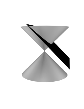
Figure 1: The null cone. In a three dimensional space of signature $(2,1)$ the set of null vectors form a cone. To ensure a unique representation of points that maintains orientation, we restrict to the subsection with positive $e_{0}$ component. The set of vectors satisfying $X\cdot n=-2$ defines the ‘standard’ representation of points, in this case defining the conformal representation of a one-dimensional space.

The power of the conformal representation starts to become clear when we consider the inner product of points. Suppose that $X$ and $Y$ are the conformal representations of the points $x$ and $y$ respectively, both in the standard form of equation (5). Their inner product is

$$X\!\cdot\!Y =\bigl{(}x^{2}n+2x-\bar{n}\bigr{)}\!\cdot\!\bigl{(}y^{2}n+2y-\bar{n}\bigr{)}$$

$$=-2x^{2}-2y^{2}+4x\!\cdot\!y$$

$$=-2(x-y)^{2}.$$ (8)

This is the essential result that underpins the conformal approach to Euclidean geometry. The inner product in conformal space encodes the distance between points in Euclidean space. This is the reason why points are represented with null vectors — the distance between a point and itself is zero.

Generalising equation (8) to unnormalised vectors, the distance between points can be written

$$|x-y|^{2}=-2\frac{X\!\cdot\!Y}{X\!\cdot\!n\,Y\!\cdot\!n}.$$ (9)

Any transformation of $X$ and $Y$ that leaves this product invariant must represent a symmetry of Euclidean space. Because such a transformation must leave the inner product invariant, it must be an orthogonal transformation in conformal space. Such a transformation ensures that null vectors remain null vectors, and so continue to represent points. The transformation must also leave $n$ invariant if the distance is to remain unchanged. We can now see that the Euclidean group is the subgroup of conformal transformations that leaves invariant the point at infinity. In what follows we will find applications for both Euclidean and more general conformal transformations.

3 Conformal Geometric Algebra

Geometric algebra was introduced by the nineteenth century mathematician W.K. Clifford, and has found many applications in physics [6, 12]. Often in this work the name Clifford algebra is used, but for applications in geometry it is becoming increasingly common to see Clifford’s original name of geometric algebra to describe the field. A geometric algebra is constructed over a vector space with a given inner product. The geometric product of two vectors $a$ and $b$ is defined to be associative and distributive over addition, with the additional rule that the square of any vector is a scalar,

$$aa=a^{2}\in\mathbb{R}.$$ (10)

If we write

$$ab+ba=(a+b)^{2}-a^{2}-b^{2}$$ (11)

we see that the symmetric part of the geometric product of any two vectors is also a scalar. This defines the inner product, and we write

$$a\!\cdot\!b={\textstyle\frac{1}{2}}(ab+ba).$$ (12)

The remaining, antisymmetric part of the geometric product returns the outer or exterior product familiar from projective geometry. We write this as

$$a\!\wedge\!b={\textstyle\frac{1}{2}}(ab-ba).$$ (13)

The totally antisymmetrised sum of geometric products of vectors defines the exterior product in the algebra.

The geometric product of two vectors can now be written

$$ab=a\!\cdot\!b+a\!\wedge\!b.$$ (14)

Under the geometric product, orthogonal vectors anticommute and parallel vectors commute. The product therefore encodes the basic geometric relationships between vectors. Now that we know how to multiply vectors together, it is straightforward to construct the entire geometric algebra of a given vector space. This is facilitated by introducing an orthonormal frame of vectors $\{e_{i}\}$. These satisfy

$$e_{i}\!\cdot\!e_{j}=\eta_{ij},$$ (15)

where $\eta_{ij}$ is the metric tensor. For a space of signature $(p,q)$, $\eta_{ij}$ is a diagonal matrix consisting of $p$ $+1$s and $q$ $-1$s. The space of interest to us here is the conformal space of signature $(4,1)$. A basis for this is provided by the vectors $e_{0},\ldots,e_{4}$, with $e_{0}$ having negative square. The algebra generated by these vectors has 32 terms in total, and is spanned by

$$\begin{array}[]{rcccccc}&1&\{e_{i}\}&\{e_{i}\!\wedge\!e_{j}\}&\{e_{i}\!\wedge\!e_{j}\!\wedge\!e_{k}\}&\{Ie_{i}\}&I\\ \mbox{grade}&0&1&2&3&4&5\\ \mbox{dimension}&1&5&10&10&5&1.\end{array}$$

We refer to this algebra as ${\mathcal{G}}(4,1)$. The term ‘grade’ is used to refer to the number of vectors in any exterior product. The dimensions of each graded subspace are given by the binomial coefficients.

The highest grade term in ${\mathcal{G}}(4,1)$ is called the pseudoscalar and is given the symbol $I$. This is defined by

$$I=e_{0}e_{1}e_{2}e_{3}e_{4}.$$ (16)

The pseudoscalar commutes with all elements in the algebra, a feature of odd-dimensional algebras, and the $(4,1)$ signature of the space implies that the pseudoscalar satisfies

$$I^{2}=-1.$$ (17)

So, algebraically, $I$ has the properties of a unit imaginary. But it also plays a definite geometric role, as multiplication by the pseudoscalar performs a duality transformation in conformal space. A matrix representation of ${\mathcal{G}}(4,1)$ can be constructed in terms of $4\times 4$ complex matrices. These can be found in the physics literature in the guise of the Dirac matrices [13]. For practical applications this matrix representation has little value and one is better off coding up the algebraic rules explicitly.

A general element of ${\mathcal{G}}(4,1)$ is called a multivector and can consist of a sum of terms all grades in the algebra. Arbitrary elements of ${\mathcal{G}}(4,1)$ can be added and multiplied together. A multivector that consists only of terms of a single grade is said to be homogeneous. The geometric product of a pair of homogeneous multivectors decomposes as follows:

$$A_{r}B_{s}=\langle A_{r}B_{s}\rangle_{|r-s|}+\langle A_{r}B_{s}\rangle_{|r-s|+2}+\cdots+\langle A_{r}B_{s}\rangle_{r+s}.$$ (18)

The angle brackets $\langle M\rangle_{r}$ are used to denote the projection onto the grade-$r$ terms in $M$. The dot and wedge symbols are used to generalise the inner and outer products to the lowest and highest grade terms in a general product:

$$A_{r}\!\cdot\!B_{s} =\langle A_{r}B_{s}\rangle_{|r-s|}$$

$$A_{r}\!\wedge\!B_{s} =\langle A_{r}B_{s}\rangle_{r+s},$$ (19)

where $A_{r}$ and $B_{s}$ are homogeneous multivectors of grade $r$ and $s$ respectively. One only ever uses the dot and wedge symbols when applied to homogeneous multivectors. Of particular importance are the inner and outer products with a vector. These satisfy

$$a\!\cdot\!A_{r} ={\textstyle\frac{1}{2}}(aA_{r}-(-1)^{r}A_{r}a)$$

$$a\!\wedge\!A_{r} ={\textstyle\frac{1}{2}}(aA_{r}+(-1)^{r}A_{r}a).$$ (20)

Some straightforward algebra confirms that the outer product is associative [6].

An important algebraic operation applied to multivectors is reversion. This plays an analogous role to transposition in matrix algebra. The reverse of a multivector $M$ is denoted by $\tilde{M}$ and is defined by reversing the order of all geometric products of vectors in $M$. An arbitrary multivector in ${\mathcal{G}}(4,1)$ can be written as

$$M=\alpha+a+B+T+Ib+I\beta$$ (21)

where $\alpha$ and $\beta$ are scalars, $a$ and $b$ are vectors, $B$ is a bivector and $T$ is a trivector. The reverse of $M$ is then given by

$$\tilde{M}=\alpha+a-B-T+Ib+I\beta.$$ (22)

A conformal transformation in the Euclidean space $\mathbb{R}^{3}$ is represented by an orthogonal transformation in ${\mathcal{G}}(4,1)$. Of particular relevance here are special conformal transformations. These have determinant $+1$, and correspond to orientation-preserving transformations on $\mathbb{R}^{3}$. In geometric algebra a special conformal transformation, applied to an arbitrary multivector $A$, can be written in the compact form

$$A\mapsto RA\tilde{R}.$$ (23)

Here $R$ is an even-grade element (grades 0, 2 and 4) satisfying

$$R\tilde{R}=1.$$ (24)

Because our representation is homogeneous, this normalisation constraint can usually be relaxed to allow for $R\tilde{R}$ to be an arbitrary positive scalar. The element $R$ is called a rotor. As an example, the (unnormalised) rotor for the Euclidean translation between $x$ and $y$ can be written

$$T_{xy}=(n\!\cdot\!Y)nX+(n\!\cdot\!X)Yn,$$ (25)

where $X$ and $Y$ are the conformal equivalents of $x$ and $y$ respectively. Every rotor can be written in term of the exponential of a bivector as

$$R=\pm\exp(-B/2).$$ (26)

The bivector $B$ is the generator of the rotation, and is an element of the Lie algebra of the conformal group.

4 Geometric primitives in conformal algebra

We have now established how points in $\mathbb{R}^{3}$ are represented by null vectors in the conformal algebra ${\mathcal{G}}(4,1)$. We now need to establish how higher dimensional objects are represented. Given a null vector $Y$, one view of the point this represents is as the solution space of the equation

$$Y\!\wedge\!X=0,\qquad X^{2}=0.$$ (27)

where here $X$ is treated as a vector variable. This is a similar idea to projective geometry, and generalises immediately to higher-grade objects. Given a multivector $A_{r}$, the outer product of $r$ distinct vectors, the geometric object that this represents is the solution space of

$$A_{r}\!\wedge\!X=0,\qquad X^{2}=0.$$ (28)

This pair of equations is clearly homogeneous in $X$. If a conformal transformation is applied to $A_{r}$, taking it to $RA_{r}\tilde{R}$, then the solution space transforms in exactly the same way (that is, $X\mapsto RX\tilde{R}$). In this manner conformal transformations are easily applied to higher-grade objects.

After vectors, the next objects to consider are bivectors. Given a bivector $B$ (formed from the outer product of two vectors), the solution space of equation (28) depends on the sign of $B^{2}$. If $B^{2}$ is negative there are no solutions, if $B^{2}=0$ there is one solution, and if $B^{2}$ is positive there are two solutions. This final case corresponds to the situation where $B=X\!\wedge\!Y$, where $X$ and $Y$ are a pair of null vectors. Given a bivector of this form it is straightforward to recover $X$ and $Y$ [6], so a bivector can encode a pair of points.

Next consider a trivector $L$. The main example of relevance is the trivector formed from the outer product of three points $X_{1}$, $X_{2}$ and $X_{3}$, so

$$L=X_{1}\!\wedge\!X_{2}\!\wedge\!X_{3}.$$ (29)

Any vector $X$ that is a solution of $L\!\wedge\!X=0$ must be a linear combination of $X_{1}$, $X_{2}$ and $X_{3}$. The fact that $X$ is null and has arbitrary scale implies that in $\mathbb{R}^{3}$ the solution space is one-dimensional. To see what this space is, consider the null vector $C$, where

$$C=LnL.$$ (30)

If $X$ satisfies $X\!\wedge\!L=0$, then $X$ commutes with $L$. It follows that

$$\frac{X\!\cdot\!C}{X\!\cdot\!n\,C\!\cdot\!n}=\frac{L^{2}}{C\!\cdot\!n}=\mbox{constant}.$$ (31)

The solution set $X$ therefore consists of points at an equal distance from some point $C$. It follows that the trivector $L$ represents the circle through $X_{1}$, $X_{2}$ and $X_{3}$. If this circle also passes through the point at infinity, the line is straight. That is, the test that a line $L$ is straight is that

$$L\!\wedge\!n=0.$$ (32)

Similarly, the straight line through $X_{1}$ and $X_{2}$ is given by

$$L=X_{1}\!\wedge\!X_{2}\!\wedge\!n.$$ (33)

Conformal algebra therefore treats lines and circles in a unified manner as trivectors in ${\mathcal{G}}(4,1)$. This is to be expected, as a conformal transformation can always transform a line into a circle.

The radius $\rho$ of the circle $L$ is found from

$$\rho^{2}=-\frac{L^{2}}{(L\!\wedge\!n)^{2}}.$$ (34)

So again we see how a metric object (the radius) is recovered from a homogeneous representation of a geometric entity (the circle $L$). The angle $\theta$ between two circles (or lines) is found from

$$\cos\theta=\frac{L_{1}\!\cdot\!L_{2}}{|L1|\,|L2|}.$$ (35)

As expected, this is invariant under the full conformal group.

Similar considerations apply to the 4-vector $S$ defined by the four points $X_{1},\ldots,X_{4}$,

$$S=X_{1}\!\wedge\!X_{2}\!\wedge\!X_{3}\!\wedge\!X_{4}.$$ (36)

The object defined by $S$ is the unique sphere through the four points (which cannot all lie on a line or circle if $S\neq 0$). The centre of the sphere is given by $SnS$, and if the centre lies at infinity the sphere reduces to a plane. As with the case of a straight line, the plane defined by the three points $X_{1}$, $X_{2}$ and $X_{3}$ is

$$P=X_{1}\!\wedge\!X_{2}\!\wedge\!X_{3}\!\wedge\!n.$$ (37)

Lines, circles, planes and spheres can all be intersected in a straightforward manner in conformal geometric algebra. The two cases of greatest significance are those of a circle and a sphere, and of two spheres. Treating the latter first, any two spheres intersect in a circle (provided they touch). This reduces to a line if both spheres are in fact planar. The intersection $L$ is found simply by

$$L=(IS_{1})\!\cdot\!S_{2},$$ (38)

which is a trivector, as required. Similarly, the intersection of a circle $C$ and a sphere $S$ is given by

$$B=(IC)\!\cdot\!S.$$ (39)

This is a bivector, as a circle can intersect a sphere or plane in zero, one, or two points. In the case where $C$ is a straight line and $S$ is a flat plane, one of the points of intersection is at infinity. As we proceed we will see how the orientations implicit in lines and surfaces are neatly encoded in these intersection formulae.

5 Circle blending

Suppose we are given a series of $n+1$ points $x_{0},\ldots,x_{n}$ and we seek a smooth curve through all of these points. The idea behind the circle blending scheme is to find a curve that is as close as possible to a circle and which passes through all of the points. A typical setup is illustrated in figure 2. Consider the four points $x_{i-1}\ldots x_{i+2}$. We form the circle $C_{i}$ through $x_{i-1}$, $x_{i}$ and $x_{i+1}$, and the circle $C_{i+1}$ through $x_{i}$, $x_{i+1}$ and $x_{i+2}$. In the region between $x_{i}$ and $x_{i+1}$ we need a curve that blends smoothly between the circles $C_{i}$ and $C_{i+1}$.

Figure 2: Circles splines in the plane. The curve through each intermediate point is generated by blending between the two circles at each end, producing a smooth curve with limited change in its curvature from point to point. The curve shown has $G_{2}$ continuity, using the scheme described in section 7.

A range of schemes exist for interpolating between circles, but one is naturally picked out from the viewpoint of conformal geometry. We are presented with two circles $C_{1}$ and $C_{2}$, both of which share two points in common:

$$C_{1} =X_{0}\!\wedge\!X_{1}\!\wedge\!X_{2}$$

$$C_{2} =X_{1}\!\wedge\!X_{2}\!\wedge\!X_{3}.$$ (40)

Given the (conformal) points $X_{1}$, $X_{2}$, and the circles $C_{1}$ and $C_{2}$, there are no further objects to specify. First we need to define family of circles between $C_{1}$ and $C_{2}$. This is easily achieved by finding the transformation between them. The transformation must map between two circles, so is a conformal transformation. The only bivector generator for such a transformation is the antisymmetrised product between $C_{1}$ and $C_{2}$. A transformation governed by this generator is simply a rotation in ${\mathcal{G}}(4,1)$. If we normalise the circles by defining

$$\hat{C_{i}}=\frac{C_{i}}{|C_{i}|}$$ (41)

then the interpolated circle is simply

$$\hat{C}_{12}(\lambda)=\frac{1}{\sin(\theta)}\left(\sin\bigl{(}(1-\lambda)\theta\bigr{)}\hat{C}_{1}+\sin(\lambda\theta)\hat{C}_{2}\right).$$ (42)

Here $\theta$ is the angle between the circles, defined by

$$\cos(\theta)=\hat{C}_{1}\!\cdot\!\hat{C}_{2}.$$ (43)

(The case of $\theta>\pi$ will be addressed shortly.) This method of interpolating between circles recovers the angle-blending scheme of Séquin & Yen [4], thus providing a firm geometric reason for preferring that scheme. At this point there is no reason for $C_{1}$ and $C_{2}$ to lie in the same plane. If they lie on different planes then the four points $X_{0},\ldots,X_{3}$ define a sphere. Since the interpolated circles can be written

$$\hat{C}_{12}(\lambda)=\frac{1}{\sin(\theta)}X_{1}\!\wedge\!X_{2}\!\wedge\!\left(\sin\bigl{(}(1-\lambda)\theta\bigr{)}\frac{X_{0}}{|C_{1}|}+\sin(\lambda\theta)\frac{X_{2}}{|C_{2}|}\right),$$ (44)

we see that all points on these circles are combinations of $X_{0}\ldots X_{3}$. It follows that all of the intermediate circles also lie of the sphere defined by $X_{0},\ldots,X_{3}$, which is a desirable property for a range of applications [5]. The basic interpolation scheme is illustrated in figure 3

Figure 3: Interpolating between a pair of circles. The two outer circles share two points in common, and between them specify a sphere. All of the intermediate circles also lie on this sphere.

Now that we have a straightforward means of encoding the circle blends, we need to parameterise the actual trajectory between the points. A simple means for achieving this is to start with the straight line between $X_{1}$ and $X_{2}$. This path is parameterised by

$$Y_{12}(\lambda)=-(1-\lambda)X_{2}\!\cdot\!n\,X_{1}-\lambda X_{1}\!\cdot\!n\,X_{2}+\lambda(1-\lambda)X_{1}\!\cdot\!X_{2}\,n,$$ (45)

and the line itself is described by

$$L_{12}=X_{1}\!\wedge\!X_{2}\!\wedge\!n.$$ (46)

The rotor that transforms between the line $L_{12}$ and the circle $C_{12}(\lambda)$ is simply

$$R_{12}(\lambda)=1+\hat{C}_{12}(\lambda)\hat{L}_{12}.$$ (47)

So once the (normalised) blended circle $\hat{C}_{12}(\lambda)$ is found, the path itself is given by transforming from the straight line to the circle. The path between $X_{1}$ and $X_{2}$ is therefore simply

$$X_{12}(\lambda)=R_{12}(\lambda)Y_{12}(\lambda)\tilde{R}_{12}(\lambda).$$ (48)

This is extremely simple to code up. We never have to calculate the centre of a circle, and the algorithm deals equally easily with straight lines or circles. The algorithm keeps all intermediate points on the sphere defined by each group of four points. If all of the base points lie on the same sphere, then we compute smooth curves over this sphere. An example of this is shown in figure 4.

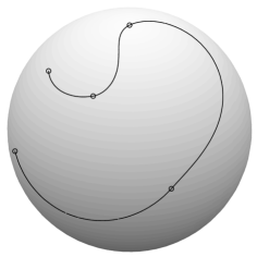
Figure 4: Circles splines on a sphere. The curve is generated using the same algorithm as for the planar case. The algorithm ensures that all intermediate points in the middle section lie on the sphere specified by the four control points. In the example, all five control points lie on the same sphere, so the curve sits smoothly on the sphere.

6 Problems and special cases

Provided the sequence of any four points are unique, the circles to be blended and the intermediate straight line are all well defined. The only aspects of the algorithm that can be problematic are concerned with the definition of the angle $\theta$ in equation (42). There are two cases over which care must be taken, both of which can be treated fairly easily. The first obvious problem is that the definition of the blended segment breaks down if $\sin(\theta)=0$, which occurs when $\cos(\theta)=+1$ and when $\cos(\theta)=-1$. The former case corresponds to $\theta=0$ and implies that the two curves are the same. This is easily caught by setting a threshold value for $\theta$ below which eqn (42) is replaced by the small-$\theta$ limit of

$$C_{12}(\lambda)=(1-\lambda)\hat{C}_{1}+\lambda\hat{C}_{2}.$$ (49)

The case of $\theta=\pi$ is more complicated, and corresponds to a somewhat pathological example. This occurs when the two circles only differ in their orientation, so $\hat{C}_{2}=-\hat{C}_{1}$. A sample configuration is shown in figure 5. All four points lie in a plane, so the interpolated curve must also lie in this plane. It is possible to define an interpolation scheme for this case. If we let $P$ denote the plane containing the circles, then the generator of the transformation must act in the $P$ plane, leaving $X_{1}$ and $X_{2}$ invariant. The bivector generator for the transformation is therefore

$$B_{12}=(X_{1}\!\wedge\!X_{2})P.$$ (50)

This produces the type of interpolated curve shown in figure 5. The problem here is that this case is not smoothly connected to the general case. Imagine moving one of the control points in figure 5 slightly out of the page. The four points then define a sphere, and the interpolated curve will lie on this sphere. This is a totally different curve to the planar case. If we are only interested in planar plots, then everything is well-behaved and the above case can be easily dealt with. But if we are interested in curves in three-dimensional space, this case is best avoided altogether with the addition of further control points.

Figure 5: Four points on a circle. The four points lie on a circle, but the two circles we interpolate between are equal and opposite. An interpolation scheme in the plane is quite possible, but the case is pathological. If one point moves slightly off the plane, the interpolated curve will jump to a spherical case.

The case of oppositely oriented circles relates to the second key issue, which is what happens if the circles are greater than $180^{\circ}$ apart? The arccos function will not return the correct angle, and the interpolation scheme will effectively blend the wrong way. This problem has an elegant solution within the conformal framework. The question reduces to finding the correct midpoint circle $C_{1,2}$. This is given by

$$C_{1,2}=\begin{cases}\hat{C}_{1}+\hat{C}_{2},\quad&\theta<\pi\\ -(\hat{C}_{1}+\hat{C}_{2}),\quad&\theta>\pi\end{cases}.$$ (51)

The case of $\theta=\pi$ corresponds to equal and opposite circles, which is the one awkward case we have to avoid. All we need is a test to decide which is the correct mid-circle for the geometry, and the arccos function can be used to determine $\theta/2$ unambiguously from

$$\cos(\theta/2)=\hat{C}_{1}\!\cdot\!\hat{C}_{1,2}.$$ (52)

To find a suitable test we consider the plane of points equidistant from $X_{1}$ and $X_{2}$. This plane is defined by

$$\Pi=I(X_{1}\!\wedge\!X_{2})\!\cdot\!n.$$ (53)

All planes are oriented, so the sign here is important. This choice corresponds to the normal to the plane (defined by the right-hand rule) pointing in the direction from $X_{1}$ to $X_{2}$. Now suppose that we intersect a circle $C$ with the plane $\Pi$. The result is two points encoded in the bivector $B$, where

$$B=I(C\Pi+\Pi C).$$ (54)

The bivector $B$ contains the points in the order

$$B=X_{f}\!\wedge\!X_{i},$$ (55)

where $X_{f}$ is the point where the circle intersects the plane from the negative to positive side, and $X_{i}$ is the opposite point (see figure 6).

Figure 6: Intersection of a plane and a circle. Both the plane and the circle are oriented objects, and the intersection bivector defined by equation (54) returns $X_{f}\!\wedge\!X_{i}$.

Now suppose that $M_{1}$ and $M_{2}$ are the midpoints of the circle segments $C_{1}$ and $C_{2}$ respectively. Both lie in the plane $\Pi$. The correct mid-circle should have its $X_{f}$ intersection point closer to the midpoint of $M_{1}$ and $M_{2}$ than its $X_{i}$ point. If this is not the case, then the circle has the wrong orientation. We therefore only need form the quantity

$$\alpha=\bigl{(}(M_{1}\!\cdot\!n\,M_{2}+M_{2}\!\cdot\!n\,M_{1})\!\wedge\!n\bigr{)}\!\cdot\!B$$ (56)

where $B$ is given by equation (54) with $C$ defined by

$$C=\hat{C}_{1}+\hat{C}_{2}.$$ (57)

The test is now

$$C_{1,2}=\begin{cases}\hat{C}_{1}+\hat{C}_{2},\quad&\alpha<0\\ -(\hat{C}_{1}+\hat{C}_{2}),\quad&\alpha>0\end{cases}.$$ (58)

This conditional statement covers all special cases (where various circles are degenerate or reduce to straight lines) and the border cases of $\alpha=0$ is the single degenerate case mentioned above. With the mid-circle found, the angle $\theta$ is computed, and the interpolation scheme of equation (42) can be followed.

A further problem with the blending scheme is highlighted in figure 7. The geometry of the control points ensures that an unwanted inversion arises in the middle of the plot. This is because the gradient at each control point is fixed entirely by the two points on either side (see section 7), and so in this case is forced to be flat, as illustrated. The problem can be removed in a number of ways. One of the simplest is to define a series of midpoints, and then repeat the blending algorithm. The result of a single iteration of this type is also shown in figure 7. Of course, one can go further and continue to recursively define midpoints, which will also generate a smooth blend. This latter approach has the attractive feature that it removes the need for any trigonometric evaluations, as the mid-circle is found easily using the method described above.

Figure 7: An unwanted inversion. The blending scheme does not always minimise curvature, and can lead to additional inversions in certain cases, as shown on the left-hand side. This is because the gradient at any point is determined entirely by the two points directly next to it. The problem can be resolved by introducing additional midpoints in the problem area and re-blending, producing the smooth curve shown on the right.

7 Continuity

An important issue in any interpolation scheme is the order of continuity at the control points. In this section we will only consider $G$-continuity. To achieve $C$-continuity some reparameterisation will have to occur on each spline. For the case of a camera fly-by, this can be achieved by specifying the desired velocity along the curve.

Our blending scheme is defined by equation (48), and before we can differentiate this we need a result for the derivative of a rotor. The definition of a (normalised) rotor is sufficient to prove that we can always write

$$\frac{\partial R}{\partial\lambda}=-{\textstyle\frac{1}{2}}RB$$ (59)

where $B$ is a bivector, which in general will also be a function of $\lambda$. (The factor of $-1/2$ is a useful convention). To find the tangent vector to the (conformal) curve $X(\lambda)$ we form the line

$$T=X\!\wedge\!X^{\prime}\!\wedge\!n$$ (60)

where the dash denotes the derivative with respect to $\lambda$. To see how this behaves we return to equation (48) and form the derivative at $\lambda=0$. For convenience we will assume that the rotor in equation (47) has been normalised, though this is unimportant when forming the tangent vector. In evaluating the derivatives we can use the results that

$$R(\lambda)X_{1}\tilde{R}(\lambda)=X_{1},\qquad R(\lambda)X_{2}\tilde{R}(\lambda)=X_{2}.$$ (61)

Differentiating these, we see that

$$X_{1}\!\cdot\!B(\lambda)=X_{2}\!\cdot\!B(\lambda)=0,$$ (62)

and these also hold for derivatives of $B$ with respect to $\lambda$.

On differentiating (47) we find that (dropping the subscripts on $R$ and $Y$)

$$X^{\prime}=R(Y\!\cdot\!B+X_{2}\!\cdot\!n\,X_{1}-X_{1}\!\cdot\!n\,X_{2}+(1-2\lambda)X_{1}\!\cdot\!X_{2}\,n)\tilde{R}.$$ (63)

It follows that

$$\left.X^{\prime}\right|_{\lambda=0}=X_{2}\!\cdot\!n\,X_{1}-X_{1}\!\cdot\!n\,X_{2}+X_{1}\!\cdot\!X_{2}\,R_{0}n\tilde{R}_{0},$$ (64)

where $R_{0}=R(\lambda=0)$. The tangent vector at $X_{1}$ is therefore given by (up to a scale factor)

$$T_{1} =X_{1}\!\cdot\!n\,X_{2}\!\wedge\!X_{1}\!\wedge\!n-X_{1}\!\cdot\!X_{2}\,(R_{0}n\tilde{R}_{0})\!\wedge\!X_{1}\!\wedge\!n$$

$$=-\Bigl{(}R_{0}\bigl{(}(X_{1}\!\wedge\!X_{2}\!\wedge\!n)\!\cdot\!X_{1}\bigr{)}\tilde{R}_{0}\Bigr{)}\!\wedge\!n$$

$$=-(C_{1}\!\cdot\!X_{1})\!\wedge\!n.$$ (65)

But this is precisely the tangent vector to the circle $C_{1}$ at that point $X_{1}$. So the tangent at each of the control points is defined by the circle through the control point and its two adjoining points. The tangent vectors at a connection are therefore continuous, which ensures $G_{1}$ continuity.

Next we need to consider $G_{2}$ continuity. For this we need the circle

$$C_{v} =X\!\wedge\!X^{\prime}\!\wedge\!X^{\prime\prime}$$

$$=R\Bigl{(}Y\!\wedge\!\bigl{(}Y^{\prime}+Y\!\cdot\!B)\!\wedge\!\bigl{(}Y^{\prime\prime}+2Y^{\prime}\!\cdot\!B+Y\!\cdot\!B^{\prime})\Bigr{)}\tilde{R}.$$ (66)

Evaluating this at $\lambda=0$ we obtain

$$C_{v} =R_{0}\,(-X_{2}\!\cdot\!n\,X_{1})\!\wedge\!(X_{2}\!\cdot\!n\,X_{1}-X_{1}\!\cdot\!n\,X_{2}+X_{1}\!\cdot\!X_{2}\,n)\wedge$$

$$\quad(-2X_{1}\!\cdot\!X_{2}\,n+2X_{1}\!\cdot\!X_{2}\,n\!\cdot\!B(0))\,\tilde{R}_{0}$$

$$=-2(X_{1}\!\cdot\!n\,X_{2}\!\cdot\!n\,X_{1}\!\cdot\!X_{2})C_{1}$$

$$\quad-2(X_{2}\!\cdot\!n\,X_{1}\!\cdot\!X_{2})\,R_{0}\,X_{1}\!\wedge\!(-X_{1}\!\cdot\!n\,X_{2}+X_{1}\!\cdot\!X_{2}\,n)\!\wedge\!(n\!\cdot\!B(0))\,\tilde{R}_{0}.$$ (67)

This contains a term in $C_{1}$, and an additional term controlled by the bivector $B$ (evaluated at $\lambda=0$). The first term is the desired one, as it ensures that the radius of curvature at the control point is defined by the circle through it. The second term is not wanted, and implies that the simple scheme defined by equation (42) does not guarantee $G_{2}$ continuity. This was first pointed out by Séquin & Lee [5]. To provide $G_{2}$ continuity we need only ensure that the derivative of the interpolating rotor $R$ vanishes at the endpoints. This is simply achieved by replacing equation (42) with

$$\hat{C}_{12}(\lambda)=\frac{1}{\sin(\theta)}\left(\sin\bigl{(}(1-3\lambda^{2}+2\lambda^{3})\theta\bigr{)}\hat{C}_{1}+\sin((3\lambda^{2}-2\lambda^{3})\theta)\hat{C}_{2}\right).$$ (68)

This blending scheme does now have $G_{2}$ continuity, and is the scheme use to produce the figures in section 5. In figure 8 we show a comparison between the two schemes. As expected, the $G_{2}$ scheme smoothes out some of the curvature around the control points. One can extend this idea to obtain any desired order of continuity. This is achieved by replacing the polynomial in equation (68) by a higher-order blend.

Figure 8: Comparison between $G_{1}$ and $G_{2}$ continuity. The $G_{1}$ blend is shown on the left, and the $G_{2}$ blend on the right. The $G_{2}$ blend hugs the control points more closely than the $G_{1}$ case, and for most cases the $G_{2}$ curves are the more aesthetically satisfying.

8 Sphere blending

One can straightforwardly apply the ideas developed here to swept surfaces using a version of the scheme described by Szilvási-Nagy & Vendel [3]. But in this section we aim to explore an alternative idea, based on sphere blending. A sphere is described as a 4-vector in the conformal geometric algebra, and these can be transformed and interpolated in a similar manner to circles.

As a simple example, suppose that the points $X_{1}$, $X_{2}$ and $X_{3}$ define the vertices of a triangle. To each corner we attach a sphere, $S_{1}$, $S_{2}$ and $S_{3}$. Each sphere passes through the three vertices of the triangle, and a fourth point which can be viewed as a control point. That is, we can write

$$S_{1} =A_{1}\!\wedge\!X_{1}\!\wedge\!X_{2}\!\wedge\!X_{3}$$

$$S_{2} =A_{2}\!\wedge\!X_{1}\!\wedge\!X_{2}\!\wedge\!X_{3}$$

$$S_{3} =A_{3}\!\wedge\!X_{1}\!\wedge\!X_{2}\!\wedge\!X_{3}.$$ (69)

These assume that none of $A_{1}$, $A_{2}$ and $A_{3}$ lie on the circle defined by $X_{1}$, $X_{2}$ and $X_{3}$. We next need to define a blend over the surface. For this we introduce the barycentric coordinates $(\lambda,\mu,\nu)$, subject to

$$0\leq\lambda,\mu,\nu\leq 1,\quad\lambda+\mu+\nu=1.$$ (70)

We let $Y(\lambda,\mu)$ denote the conformal representation of the point in the triangle corresponding to the barycentric coordinates $(\lambda,\mu,1-\lambda-\mu)$. Similarly, we define a (linear) sphere blend by

$$S(\lambda,\mu)=\lambda\hat{S}_{1}+\mu\hat{S}_{2}+\nu\hat{S}_{3}.$$ (71)

We could employ a trigonometric blending scheme over the (abstract) sphere defined by the unit 4-vectors $\hat{S}_{1}$, $\hat{S}_{2}$ and $\hat{S}_{1}$, but this raises a number of complications. There is no single straightforward generalisation of barycentric coordinates over a spherical triangle, and each alternative scheme has its own merits and drawbacks [14]. Here we have adopted the simplest, linear blending scheme, which generates interesting surfaces.

Now that we have the sphere and the point on the triangle defined, all that remains is to define the conformal transformation from the point to the blended surface. First we define the plane $P$ through the three base points,

$$P=X_{1}\!\wedge\!X_{2}\!\wedge\!X_{3}\!\wedge\!n.$$ (72)

Next we define the rotor $R$ for the conformal transformation between the plane and the blended sphere,

$$R(\lambda,\mu)=1-\hat{S}(\lambda,\mu)\hat{P}.$$ (73)

Finally, the surface itself is defined by the points $X(\lambda,\mu)$, where

$$X(\lambda,\mu)=R(\lambda,\mu)Y(\lambda,\mu)\tilde{R}(\lambda,\mu).$$ (74)

A typical surface defined in this manner is shown in figure 9. The result is aesthetically quite pleasing, yielding a smooth blend free of sudden changes in curvature.

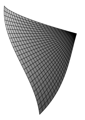
Figure 9: A blended surface. A sphere is attached to each of the vertices of a triangle. The surface is defined by a linear blend of the spheres.

Much work remains to extend this idea to a complete framework for defining blends over surfaces. The control points need to be chosen so as to reflect the geometry around the triangle, and continuity between blended spheres may be hard to achieve. Here we hope to have demonstrated that such an approach may be feasible.

9 Summary

Smooth splines between control points can be defined in terms of blended circles. The splines pass through all points, and have no extra control points. The natural geometric framework for handling circles is conformal geometry. This geometry is encapsulated in a simple, unified manner by employing the geometric algebra of a five-dimensional space. All transformations are easily defined, and algorithms can be written in such a way as to minimise problems with special cases. Similar ideas can be applied to sphere blends over a surface, and in future work we will explore the potential of this idea for design and for encoding surface data.

References

- [1] H.P. Moreton and C.H. Séquin. Functional optimisation for fair surface design. Proc. ACM SIGGRAPH, pages 167–176, 1992.
- [2] H. Wenz. Interpolation of curve data by blended generalized circles. Computer Aided Geometric Design, 13:673–680, 1996.
- [3] M. Szivási-Nagy and T.P. Vendel. Generating curves and swept surfaces by blended circles. Computer Aided Geometric Design, 17:197–206, 2000.
- [4] C.H. Séquin and J.A. Yen. Fair and robust curve interpolation on the sphere, 2001. SIGGRAPH’01, Sketches and Applications.
- [5] C.H. Séquin and K. Lee. Fair and robust circle splines, 2003. SIGGRAPH’03, Sketches and Applications.
- [6] C.J.L Doran and A.N. Lasenby. Geometric Algebra for Physicists. Cambridge University Press, 2003.
- [7] C. Doran, A. Lasenby, and J. Lasenby. Conformal geometry, Euclidean space and geometric algebra. In J. Winkler and M. Niranjan, editors, Uncertainty in Geometric Computations, pages 41–58. Kluwer Academic Publishers, Boston, 2002.
- [8] A.N. Lasenby and J. Lasenby. Surface evolution and representation using geometric algebra. In R. Cippola, editor, The Mathematics of Surfaces IX: Proceedings of the Ninth IMA Conference on the Mathematics of Surfaces, pages 144–168. London, 2000.
- [9] L. Dorst, C. Doran, and J. Lasenby. Applications of Geometric Algebra in Computer Science and Engineering 2001. Birkhäuser, New York, 2001.
- [10] A. Rockwood, et al. Geometric algebra: New foundations, new insights, 2000. SIGGRAPH’00, Course 31.
- [11] A. Naeve, et al. Geometric algebra, 2001. SIGGRAPH’01, Course 53.
- [12] D. Hestenes. New Foundations for Classical Mechanics (Second Edition). Kluwer Academic Publishers, Dordrecht, 1999.
- [13] C. Itzykson and J-B. Zuber. Quantum Field Theory. McGraw–Hill, New York, 1980.
- [14] E. Praun and H. Hoppe. Spherical parametrization and remeshing. ACM Transactions on Graphics, 22(3):340–349, 2003.