TR IDSIA-19-03, Version 5
December 2006, arXiv:cs.LO/0309048 v5
(v1: 25 September 2003)

Gödel Machines: Self-Referential
Universal Problem Solvers Making
Provably Optimal Self-Improvements

Jürgen Schmidhuber

IDSIA, Galleria 2, 6928 Manno-Lugano, Switzerland &
TU München, Boltzmannstr. 3, 85748 Garching, München, Germany

juergen@idsia.ch - http://www.idsia.ch/~juergen

We present the first class of mathematically rigorous, general, fully self-referential, self-improving, optimally efficient problem solvers. Inspired by Kurt Gödel’s celebrated self-referential formulas (1931), such a problem solver rewrites any part of its own code as soon as it has found a proof that the rewrite is useful, where the problem-dependent utility function and the hardware and the entire initial code are described by axioms encoded in an initial proof searcher which is also part of the initial code. The searcher systematically and in an asymptotically optimally efficient way tests computable proof techniques (programs whose outputs are proofs) until it finds a provably useful, computable self-rewrite. We show that such a self-rewrite is globally optimal—no local maxima!—since the code first had to prove that it is not useful to continue the proof search for alternative self-rewrites. Unlike Hutter’s previous non-self-referential methods based on hardwired proof searchers, ours not only boasts an optimal order of complexity but can optimally reduce any slowdowns hidden by the $O()$-notation, provided the utility of such speed-ups is provable at all.

Keywords: self-reference, reinforcement learning, problem solving, proof techniques, optimal universal search, self-improvement

Gödel machine publications up to 2006 (100 years after Kurt Gödel’s birth, and 75 years after his landmark paper [11] laying the foundations of theoretical computer science): [45, 47, 48, 49, 50, 51].

1 Introduction and Outline

All traditional algorithms for problem solving / machine learning / reinforcement learning [20] are hardwired. Some are designed to improve some limited type of policy through experience, but are not part of the modifiable policy, and cannot improve themselves in a theoretically sound way. Humans are needed to create new / better problem solving algorithms and to prove their usefulness under appropriate assumptions.

Here we will eliminate the restrictive need for human effort in the most general way possible, leaving all the work including the proof search to a system that can rewrite and improve itself in arbitrary computable ways and in a most efficient fashion. To attack this “Grand Problem of Artificial Intelligence” [46], we introduce a novel class of optimal, fully self-referential [11] general problem solvers called Gödel machines [45, 47, 49, 51, 50]. They are universal problem solving systems that interact with some (partially observable) environment and can in principle modify themselves without essential limits apart from the limits of computability. Their initial algorithm is not hardwired; it can completely rewrite itself, but only if a proof searcher embedded within the initial algorithm can first prove that the rewrite is useful, given a formalized utility function reflecting computation time and expected future success (e.g., rewards). We will see that self-rewrites due to this approach are actually globally optimal (Theorem 4.1, Section 4), relative to Gödel’s well-known fundamental restrictions of provability [11]. These restrictions should not worry us; if there is no proof of some self-rewrite’s utility, then humans cannot do much either.

The initial proof searcher is $O()$-optimal (has an optimal order of complexity) in the sense of Theorem 5.1, Section 5. Unlike hardwired systems such as Hutter’s [16, 17] and Levin’s [24, 26] (Section 6.4), however, a Gödel machine can in principle speed up any part of its initial software, including its proof searcher, to meet arbitrary formalizable notions of optimality beyond those expressible in the $O()$-notation. Our approach yields the first theoretically sound, fully self-referential, optimal, general problem solvers.

Outline. Section 2 presents basic concepts and fundamental limitations, Section 3 the essential details of a self-referential axiomatic system, Section 4 the Global Optimality Theorem 4.1, and Section 5 the $O()$-optimal (Theorem 5.1) initial proof searcher. Section 6 provides examples and relations to previous work, briefly discusses issues such as a technical justification of consciousness, and lists answers to several frequently asked questions about Gödel machines.

2 Overview / Basic Ideas / Limitations

Many traditional problems of computer science require just one problem-defining input at the beginning of the problem solving process. For example, the initial input may be a large integer, and the goal may be to factorize it. In what follows, however, we will also consider the more general case where the problem solution requires interaction with a dynamic, initially unknown environment that produces a continual stream of inputs and feedback signals, such as in autonomous robot control tasks, where the goal may be to maximize expected cumulative future reward [20]. This may require the solution of essentially arbitrary problems (examples in Section 6.2 formulate traditional problems as special cases).

2.1 Set-up and Formal Goal

Our hardware (e.g., a universal or space-bounded Turing machine [61] or the abstract model of a personal computer) has a single life which consists of discrete cycles or time steps $t=1,2,\ldots$. Its total lifetime $T$ may or may not be known in advance. In what follows, the value of any time-varying variable $Q$ at time $t$ will be denoted by $Q(t)$.

During each cycle our hardware executes an elementary operation which affects its variable state $s\in\cal S\subset B^{*}$ (without loss of generality, $B^{*}$ is the set of possible bitstrings over the binary alphabet $B=\{0,1\}$) and possibly also the variable environmental state $Env\in\cal E$ (here we need not yet specify the problem-dependent set $\cal E$). There is a hardwired state transition function $F:\cal S\times\cal E\rightarrow\cal S$. For $t>1$, $s(t)=F(s(t-1),Env(t-1))$ is the state at a point where the hardware operation of cycle $t-1$ is finished, but the one of $t$ has not started yet. $Env(t)$ may depend on past output actions encoded in $s(t-1)$ and is simultaneously updated or (probabilistically) computed by the possibly reactive environment.

In order to talk conveniently about programs and data, we will often attach names to certain string variables encoded as components or substrings of $s$. Of particular interest are the three variables called time, x, y, and p:

1. At time $t$, variable $time$ holds a unique binary representation of $t$. We initialize $time(1)=`1\textrm{'}$, the bitstring consisting only of a one. The hardware increments $time$ from one cycle to the next. This requires at most $O(log~{}t)$ and on average only $O(1)$ computational steps.

2. Variable x holds the inputs from the environment to the Gödel machine. For $t>1$, $x(t)$ may differ from $x(t-1)$ only if a program running on the Gödel machine has executed a special input-requesting instruction at time $t-1$. Generally speaking, the delays between successive inputs should be sufficiently large so that programs can perform certain elementary computations on an input, such as copying it into internal storage (a reserved part of $s$) before the next input arrives.

3. Variable y holds the outputs of the Gödel machine. $y(t)$ is an output bitstring which may subsequently influence the environment, where $y(1)=`0\textrm{'}$ by default. For example, $y(t)$ could be interpreted as a control signal for an environment-manipulating robot whose actions may have an effect on future inputs.

4. $p(1)$ is the initial software: a program implementing the original (sub-optimal) policy for interacting with the environment, represented as a substring $e(1)$ of $p(1)$, plus the original policy for searching proofs. Details will be discussed below.

At any given time $t$ ($1\leq t\leq T$) the goal is to maximize future success or utility. A typical “value to go” utility function is of the form $u(s,Env):\cal S\times\cal E\rightarrow R$, where $\cal R$ is the set of real numbers:

$$u(s,Env)=E_{\mu}\left[\sum_{\tau=time}^{T}r(\tau)~{}~{}\Bigg{|}~{}~{}s,Env\right],$$ (1)

where $r(t)$ is a real-valued reward input (encoded within $s(t)$) at time $t$, $E_{\mu}(\cdot\mid\cdot)$ denotes the conditional expectation operator with respect to some possibly unknown distribution $\mu$ from a set $M$ of possible distributions ($M$ reflects whatever is known about the possibly probabilistic reactions of the environment), and the above-mentioned $time=time(s)$ is a function of state $s$ which uniquely identifies the current cycle. Note that we take into account the possibility of extending the expected lifespan through appropriate actions.

Alternative formalizable utility functions could favor improvement of worst case instead of expected future performance, or higher reward intake per time interval etc. Clearly, most classic problems of computer science can be formulated in this framework—see examples in Section 6.2.

2.2 Basic Idea of Gödel Machine

Our machine becomes a self-referential [11] Gödel machine by loading it with a particular form of machine-dependent, self-modifying code $p$. The initial code $p(1)$ at time step 1 includes a (typically sub-optimal) problem solving subroutine $e(1)$ for interacting with the environment, such as any traditional reinforcement learning algorithm [20], and a general proof searcher subroutine (Section 5) that systematically makes pairs (switchprog, proof) (variable substrings of $s$) until it finds a proof of a target theorem which essentially states: ‘the immediate rewrite of p through current program switchprog on the given machine implies higher utility than leaving p as is’. Then it executes switchprog, which may completely rewrite $p$, including the proof searcher. Section 3 will explain details of the necessary initial axiomatic system $\cal A$ encoded in $p(1)$. Compare Fig. 1.

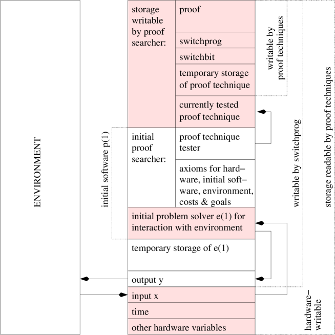
Figure 1: Storage snapshot of a not yet self-improved example Gödel machine, with the initial software still intact. See text for details.

The Global Optimality Theorem (Theorem 4.1, Section 4) shows this self-improvement strategy is not greedy: since the utility of ‘leaving $p$ as is’ implicitly evaluates all possible alternative switchprogs which an unmodified $p$ might find later, we obtain a globally optimal self-change—the current switchprog represents the best of all possible relevant self-changes, relative to the given resource limitations and initial proof search strategy.

2.3 Proof Techniques and an $O()$-Optimal Initial Proof Searcher

Section 5 will present an $O()$-optimal initialization of the proof searcher, that is, one with an optimal order of complexity (Theorem 5.1). Still, there will remain a lot of room for self-improvement hidden by the $O()$-notation. The searcher uses an online extension of Universal Search [24, 26] to systematically test online proof techniques, which are proof-generating programs that may read parts of state $s$ (similarly, mathematicians are often more interested in proof techniques than in theorems). To prove target theorems as above, proof techniques may invoke special instructions for generating axioms and applying inference rules to prolong the current proof by theorems. Here an axiomatic system $\cal A$ encoded in $p(1)$ includes axioms describing (a) how any instruction invoked by a program running on the given hardware will change the machine’s state $s$ (including instruction pointers etc.) from one step to the next (such that proof techniques can reason about the effects of any program including the proof searcher), (b) the initial program $p(1)$ itself (Section 3 will show that this is possible without introducing circularity), (c) stochastic environmental properties, (d) the formal utility function $u$, e.g., equation (1), which takes into account computational costs of all actions including proof search.

2.4 Limitations of Gödel Machines

The fundamental limitations are closely related to those first identified by Gödel’s celebrated paper on self-referential formulae [11]. Any formal system that encompasses arithmetics (or ZFC etc) is either flawed or allows for unprovable but true statements. Hence even a Gödel machine with unlimited computational resources must ignore those self-improvements whose effectiveness it cannot prove, e.g., for lack of sufficiently powerful axioms in $\cal A$. In particular, one can construct pathological examples of environments and utility functions that make it impossible for the machine to ever prove a target theorem. Compare Blum’s speed-up theorem [3, 4] based on certain incomputable predicates. Similarly, a realistic Gödel machine with limited resources cannot profit from self-improvements whose usefulness it cannot prove within its time and space constraints.

Nevertheless, unlike previous methods, it can in principle exploit at least the provably good speed-ups of any part of its initial software, including those parts responsible for huge (but problem class-independent) slowdowns ignored by the earlier approaches [16, 17] (Section 6.4).

3 Essential Details of One Representative Gödel Machine

Notation. Unless stated otherwise or obvious, throughout the paper newly introduced variables and functions are assumed to cover the range implicit in the context. $l(q)$ denotes the number of bits in a bitstring $q$; $q_{n}$ the $n$-th bit of $q$; $\lambda$ the empty string (where $l(\lambda)=0$); $q_{m:n}=\lambda$ if $m>n$ and $q_{m}q_{m+1}\ldots q_{n}$ otherwise (where $q_{0}:=q_{0:0}:=\lambda$).

Theorem proving requires an axiom scheme yielding an enumerable set of axioms of a formal logic system $\cal A$ whose formulas and theorems are symbol strings over some finite alphabet that may include traditional symbols of logic (such as $\rightarrow,\wedge,=,(,),\forall,\exists,\ldots$, $c_{1},c_{2},\ldots,$ $f_{1},f_{2},\ldots$), probability theory (such as $E(\cdot)$, the expectation operator), arithmetics ($+,-,/,=,\sum,<,\ldots$), string manipulation (in particular, symbols for representing any part of state $s$ at any time, such as $s_{7:88}(5555)$). A proof is a sequence of theorems, each either an axiom or inferred from previous theorems by applying one of the inference rules such as modus ponens combined with unification, e.g., [10].

The remainder of this paper will omit standard knowledge to be found in any proof theory textbook. Instead of listing all axioms of a particular $\cal A$ in a tedious fashion, we will focus on the novel and critical details: how to overcome potential problems with self-reference and how to deal with the potentially delicate online generation of proofs that talk about and affect the currently running proof generator itself.

3.1 Proof Techniques

Brute force proof searchers (used in Hutter’s work [16, 17]; see Section 6.4 for a review) systematically generate all proofs in order of their sizes. To produce a certain proof, this takes time exponential in proof size. Instead our $O()$-optimal $p(1)$ will produce many proofs with low algorithmic complexity [57, 22, 27] much more quickly. It systematically tests (see Section 5) programs called proof techniques written in universal language $\cal L$ implemented within $p(1)$. For example, $\cal L$ may be a variant of PROLOG [7] or the universal Forth[29]-inspired programming language used in recent work on optimal search [48]. A proof technique is composed of instructions that allow any part of $s$ to be read, such as inputs encoded in variable $x$ (a substring of $s$) or the code of $p(1)$. It may write on $s^{p}$, a part of $s$ reserved for temporary results. It also may rewrite switchprog, and produce an incrementally growing proof placed in the string variable proof stored somewhere in $s$. proof and $s^{p}$ are reset to the empty string at the beginning of each new proof technique test. Apart from standard arithmetic and function-defining instructions [48] that modify $s^{p}$, the programming language $\cal L$ includes special instructions (details in Section 3.2) for prolonging the current proof by correct theorems, for setting switchprog, and for checking whether a provably optimal $p$-modifying program was found and should be executed now. Certain long proofs can be produced by short proof techniques.

3.2 Important Instructions Used by Proof Techniques

The nature of the six proof-modifying instructions below (there are no others) makes it impossible to insert an incorrect theorem into proof, thus trivializing proof verification. Let us first provide a brief overview of the most important instructions: get-axiom(n) appends the $n$-th possible axiom to the current proof, apply-rule(k, m, n) applies the $k$-th inference rule to the $m$-th and $n$-th theorem in the current proof (appending the result), set-switchprog(m,n) sets $switchprog:=s^{p}_{m:n}$, and check() tests whether the last theorem in proof is a target theorem showing that a self-rewrite through switchprog would be useful. The details are as follows.

1. get-axiom(n) takes as argument an integer $n$ computed by a prefix of the currently tested proof technique with the help of arithmetic instructions such as those used in previous work [48]. Then it appends the $n$-th axiom (if it exists, according to the axiom scheme below) as a theorem to the current theorem sequence in proof. The initial axiom scheme encodes:

   1. Hardware axioms describing the hardware, formally specifying how certain components of $s$ (other than environmental inputs $x$) may change from one cycle to the next.

      For example, if the hardware is a Turing machine (TM) [61], then $s(t)$ is a bitstring that encodes the current contents of all tapes of the TM, the positions of its scanning heads, and the current internal state of the TM’s finite state automaton, while $F$ specifies the TM’s look-up table which maps any possible combination of internal state and bits above scanning heads to a new internal state and an action such as: replace some head’s current bit by 1/0, increment (right shift) or decrement (left shift) some scanning head, read and copy next input bit to cell above input tape’s scanning head, etc.

      Alternatively, if the hardware is given by the abstract model of a modern microprocessor with limited storage, $s(t)$ will encode the current storage contents, register values, instruction pointers etc.

      For instance, the following axiom could describe how some 64-bit hardware’s instruction pointer stored in $s_{1:64}$ is continually incremented as long as there is no overflow and the value of $s_{65}$ does not indicate that a jump to some other address should take place:

      $$(\forall t\forall n:[(n<2^{64}-1)\wedge(n>0)\wedge(t>1)\wedge(t<T)$$

      $$\wedge(string2num(s_{1:64}(t))=n)\wedge(s_{65}(t)=`0\textrm{'})]$$

      $$\rightarrow(string2num(s_{1:64}(t+1))=n+1))$$

      Here the semantics of used symbols such as ‘(’ and ‘$>$’ and ‘$\rightarrow$’ (implies) are the traditional ones, while ‘$string2num$’ symbolizes a function translating bitstrings into numbers. It is clear that any abstract hardware model can be fully axiomatized in a similar way.

   2. Reward axioms defining the computational costs of any hardware instruction, and physical costs of output actions, such as control signals $y(t)$ encoded in $s(t)$. Related axioms assign values to certain input events (encoded in variable $x$, a substring of $s$) representing reward or punishment (e.g., when a Gödel machine-controlled robot bumps into an obstacle). Additional axioms define the total value of the Gödel machine’s life as a scalar-valued function of all rewards (e.g., their sum) and costs experienced between cycles $1$ and $T$, etc. For example, assume that $s_{17:18}$ can be changed only through external inputs; the following example axiom says that the total reward increases by 3 whenever such an input equals ‘11’ (unexplained symbols carry the obvious meaning):

      $$(\forall t_{1}\forall t_{2}:[(t_{1}<t_{2})\wedge(t_{1}\geq 1)\wedge(t_{2}\leq T)\wedge(s_{17:18}(t_{2})=`11\textrm{'})]$$

      $$\rightarrow[R(t_{1},t_{2})=R(t_{1},t_{2}-1)+3]),$$

      where $R(t_{1},t_{2})$ is interpreted as the cumulative reward between times $t_{1}$ and $t_{2}$. It is clear that any formal scheme for producing rewards can be fully axiomatized in a similar way.

   3. Environment axioms restricting the way the environment will produce new inputs (encoded within certain substrings of $s$) in reaction to sequences of outputs $y$ encoded in $s$. For example, it may be known in advance that the environment is sampled from an unknown probability distribution $\mu$ contained in a given set $M$ of possible distributions (compare equation 1). E.g., $M$ may contain all distributions that are computable, given the previous history [57, 58, 16], or at least limit-computable [41, 42]. Or, more restrictively, the environment may be some unknown but deterministic computer program [63, 39] sampled from the Speed Prior [43] which assigns low probability to environments that are hard to compute by any method. Or the interface to the environment is Markovian [35], that is, the current input always uniquely identifies the environmental state—a lot of work has already been done on this special case [33, 2, 60]. Even more restrictively, the environment may evolve in completely predictable fashion known in advance. All such prior assumptions are perfectly formalizable in an appropriate $\cal A$ (otherwise we could not write scientific papers about them).

   4. Uncertainty axioms; string manipulation axioms: Standard axioms for arithmetics and calculus and probability theory [21] and statistics and string manipulation that (in conjunction with the hardware axioms and environment axioms) allow for constructing proofs concerning (possibly uncertain) properties of future values of $s(t)$ as well as bounds on expected remaining lifetime / costs / rewards, given some time $\tau$ and certain hypothetical values for components of $s(\tau)$ etc. An example theorem saying something about expected properties of future inputs $x$ might look like this:

      $$(\forall t_{1}\forall\mu\in M:[(1\leq t_{1})\wedge(t_{1}+15597<T)\wedge(s_{5:9}(t_{1})=`01011\textrm{'})$$

      $$\wedge(x_{40:44}(t_{1})=`00000\textrm{'})]\rightarrow(\exists t:[(t_{1}<t<t_{1}+15597)$$

      $$\wedge(P_{\mu}(x_{17:22}(t)=`011011\textrm{'}\mid s(t_{1}))>\frac{998}{1000})])),$$

      where $P_{\mu}(.\mid.)$ represents a conditional probability with respect to an axiomatized prior distribution $\mu$ from a set of distributions $M$ described by the environment axioms (Item 1c).

      Given a particular formalizable hardware (Item 1a) and formalizable assumptions about the possibly probabilistic environment (Item 1c), obviously one can fully axiomatize everything that is needed for proof-based reasoning about past and future machine states.

   5. Initial state axioms: Information about how to reconstruct the initial state $s(1)$ or parts thereof, such that the proof searcher can build proofs including axioms of the type

      $$(s_{{\bf m}:{\bf n}}(1)={\bf z}),~{}e.g.:~{}(s_{7:9}(1)=`010\textrm{'}).$$

      Here and in the remainder of the paper we use bold font in formulas to indicate syntactic place holders (such as m,n,z) for symbol strings representing variables (such as m,n,z) whose semantics are explained in the text—in the present context $z$ is the bitstring $s_{m:n}(1)$.

      Note that it is no fundamental problem to fully encode both the hardware description and the initial hardware-describing $p$ within $p$ itself. To see this, observe that some software may include a program that can print the software.

   6. Utility axioms describing the overall goal in the form of utility function $u$; e.g., equation (1) in Section 2.1.

2. apply-rule(k, m, n) takes as arguments the index $k$ (if it exists) of an inference rule such as modus ponens (stored in a list of possible inference rules encoded within $p(1)$) and the indices $m,n$ of two previously proven theorems (numbered in order of their creation) in the current proof. If applicable, the corresponding inference rule is applied to the addressed theorems and the resulting theorem appended to proof. Otherwise the currently tested proof technique is interrupted. This ensures that proof is never fed with invalid proofs.

3. delete-theorem(m) deletes the $m$-th theorem in the currently stored proof, thus freeing storage such that proof-storing parts of $s$ can be reused and the maximal proof size is not necessarily limited by storage constraints. Theorems deleted from proof, however, cannot be addressed any more by apply-rule to produce further prolongations of proof.

4. set-switchprog(m,n) replaces $switchprog$ by $s^{p}_{m:n}$, provided that $s^{p}_{m:n}$ is indeed a non-empty substring of $s^{p}$, the storage writable by proof techniques.

5. check() verifies whether the goal of the proof search has been reached. First it tests whether the last theorem (if any) in proof has the form of a target theorem. A target theorem states that given the current axiomatized utility function $u$ (Item 1f), the utility of a switch from $p$ to the current switchprog would be higher than the utility of continuing the execution of $p$ (which would keep searching for alternative switchprogs). Target theorems are symbol strings (encoded in $s$) of the (decoded) form

   $$(u[s({\bf t_{1}})\oplus(switchbit({\bf t_{1}})=`1\textrm{'}),Env({\bf t_{1}})]>$$

   $$u[s({\bf t_{1}})\oplus(switchbit({\bf t_{1}})=`0\textrm{'}),Env({\bf t_{1}})])$$ (2)

   where the variable $t_{1}$ (represented by syntactic place holder ${\bf t_{1}}$) stands for a time step, while all other symbols belong to the alphabet of the theorem-proving calculus, that is, the set of possible target theorems is parameterized only by $t_{1}$. Here the calculus should permit the notation $s({\bf t_{1}})\oplus(switchbit({\bf t_{1}})=`b\textrm{'})$ as a shortcut for the state obtained when we replace switchbit($t_{1}$), the true value of the variable bit $switchbit$ (encoded in $s$) at time $t_{1}$, by $b\in\{0,1\}$. This will facilitate the formulation of theorems that compare values conditioned on various alternative hypothetical properties of $s(t_{1})$. (Note that $s(t_{1})$ may be only partially known by the current proof technique even in environments where $s(t_{1})$ and switchbit($t_{1}$) are fully predetermined for all valid $t_{1}$.)

   The purpose of introducing $t_{1}$ is to deal with hardware-specific temporal delays that may be involved in checking and switching—it may take a significant amount of time to match abstract symbol strings found during proof search to the Gödel machine’s real current state. If a target theorem has been found, check() uses a simple prewired subroutine (also encoded in $p(1)$, of course) to check whether there is enough time left to set variable switchbit (originally 0) to 1 before the continually increasing $time$ will equal $t_{1}$. If this subroutine returns a negative result, check() exits. Otherwise it sets switchbit $:=1$ (there is no other way of changing switchbit). Then it repeatedly tests $time$ until $time>t_{1}$, to make sure the condition of formula (5) was fulfilled at $t_{1}$. Then it transfers control to switchprog (there is no other way of calling switchprog). The switchprog may subsequently rewrite all parts of $s$, excluding hardware-reserved parts such as $time$ and $x$, but including $p$.

6. state2theorem(m, n) takes two integer arguments $m,n$ and tries to transform the current contents of $s_{m:n}$ into a theorem of the form

   $$(s_{{\bf m}:{\bf n}}({\bf t_{1}})={\bf z}),~{}e.g.:~{}(s_{6:9}(7775555)=`1001\textrm{'}),$$

   where $t_{1}$ represents a time measured (by checking time) shortly after state2theorem was invoked, and $z$ the bistring $s_{m:n}(t_{1})$ (recall the special case $t_{1}=1$ of Item 1e). So we accept the time-labeled current observable contents of any part of $s$ as a theorem that does not have to be proven in an alternative way from, say, the initial state $s(1)$, because the computation so far has already demonstrated that the theorem is true. Thus we may exploit information conveyed by environmental inputs, and the fact that sometimes (but not always) the fastest way to determine the output of a program is to run it.

   This non-traditional online interface between syntax and semantics requires special care though. We must avoid inconsistent results through parts of $s$ that change while being read. For example, the present value of a quickly changing instruction pointer IP (continually updated by the hardware) may be essentially unreadable in the sense that the execution of the reading subroutine itself will already modify IP many times. For convenience, the (typically limited) hardware could be set up such that it stores the contents of fast hardware variables every $c$ cycles in a reserved part of $s$, such that an appropriate variant of state2theorem() could at least translate certain recent values of fast variables into theorems. This, however, will not abolish all problems associated with self-observations. For example, the $s_{m:n}$ to be read might also contain the reading procedure’s own, temporary, constantly changing string pointer variables, etc. To address such problems on computers with limited memory, state2theorem first uses some fixed protocol (encoded in $p(1)$, of course) to check whether the current $s_{m:n}$ is readable at all or whether it might change if it were read by the remaining code of state2theorem. If so, or if $m,n,$ are not in the proper range, then the instruction has no further effect. Otherwise it appends an observed theorem of the form $(s_{{\bf m}:{\bf n}}({\bf t_{1}})={\bf z})$ to proof. For example, if the current time is 7770000, then the invocation of state2theorem(6,9) might return the theorem $(s_{6:9}(7775555)=`1001\textrm{'})$, where $7775555-7770000=5555$ reflects the time needed by state2theorem to perform the initial check and to read leading bits off the continually increasing $time$ (reading $time$ also costs time) such that it can be sure that $7775555$ is a recent proper time label following the start of state2theorem.

The axiomatic system $\cal A$ is a defining parameter of a given Gödel machine. Clearly, $\cal A$ must be strong enough to permit proofs of target theorems. In particular, the theory of uncertainty axioms (Item 1d) must be sufficiently rich. This is no fundamental problem: we simply insert all traditional axioms of probability theory [21].

4 Global Optimality Theorem

Intuitively, at any given time $p$ should execute some self-modification algorithm (via instruction check()—Item 5 above) only if it is the ‘best’ of all possible self-modifications, given the utility function, which typically depends on available resources, such as storage size and remaining lifetime. At first glance, however, target theorem (5) seems to implicitly talk about just one single modification algorithm, namely, switchprog$(t_{1})$ as set by the systematic proof searcher at time $t_{1}$. Isn’t this type of local search greedy? Couldn’t it lead to a local optimum instead of a global one? No, it cannot, according to the following global optimality theorem.

4.1 Globally Optimal Self-Changes, Given $u$ and $\cal A$ Encoded in $p$

Theorem 4.1

Given any formalizable utility function $u$ (Item 1f), and assuming consistency of the underlying formal system $\cal A$, any self-change of $p$ obtained through execution of some program switchprog identified through the proof of a target theorem (5) is globally optimal in the following sense: the utility of starting the execution of the present switchprog is higher than the utility of waiting for the proof searcher to produce an alternative switchprog later.

Proof. Target theorem (5) implicitly talks about all the other switchprogs that the proof searcher could produce in the future. To see this, consider the two alternatives of the binary decision: (1) either execute the current switchprog (set switchbit $=1$), or (2) keep searching for proofs and switchprogs (set switchbit $=0$) until the systematic searcher comes up with an even better switchprog. Obviously the second alternative concerns all (possibly infinitely many) potential switchprogs to be considered later. That is, if the current switchprog were not the ‘best’, then the proof searcher would not be able to prove that setting switchbit and executing switchprog will cause higher expected reward than discarding switchprog, assuming consistency of $\cal A$. Q.E.D.

The initial proof searcher of Section 5 already generates all possible proofs and switchprogs in $O()$-optimal fashion. Nevertheless, since it is part of $p(1)$, its proofs can speak about the proof searcher itself, possibly triggering proof searcher rewrites resulting in better than merely $O()$-optimal performance.

4.2 Alternative Relaxed Target Theorem

We may replace the target theorem (5) (Item 5) by the following alternative target theorem:

$$(u[s({\bf t_{1}})\oplus(switchbit({\bf t_{1}})=`1\textrm{'}),Env({\bf t_{1}})]\geq$$

$$u[s({\bf t_{1}})\oplus(switchbit({\bf t_{1}})=`0\textrm{'}),Env({\bf t_{1}})])$$ (3)

The only difference to the original target theorem (5) is that the “$>$” sign became a “$\geq$” sign. That is, the Gödel machine will change itself as soon as it has found a proof that the change will not make things worse. A Global Optimality Theorem similar to Theorem 4.1 holds; simply replace the last phrase in Theorem 4.1 by: the utility of starting the execution of the present switchprog is at least as high as the utility of waiting for the proof searcher to produce an alternative switchprog later.

4.3 Global Optimality and Recursive Meta-Levels

One of the most important aspects of our fully self-referential set-up is the following. Any proof of a target theorem automatically proves that the corresponding self-modification is good for all further self-modifications affected by the present one, in recursive fashion. In that sense all possible “meta-levels” of the self-referential system are collapsed into one.

4.4 How Difficult is it to Prove Target Theorems?

This depends on the tasks and the initial axioms $\cal A$, of course. It is straight-forward to devise simple tasks and corresponding consistent $\cal A$ such that there are short and trivial proofs of target theorems.

Even when we initialize the initial problem solver $e(1)$ by an asymptotically optimal, rather general method such as Hutter’s Aixi(t,l) [16, 19], it may be straight-forward to prove that switching to another strategy is useful, especially when $\cal A$ contains additional prior knowledge in form of axiomatic assumptions beyond those made by Aixi(t,l). The latter needs a very time-consuming but constant set-up phase whose costs disappear in the $O()$-notation but not in a utility function such as the $u$ of equation (1). For example, simply construct an environment where maximal reward is achieved by performing a never-ending sequence of simple but rewarding actions, say, repeatedly pressing a lever, plus a very simple axiomatic system $\cal A$ that permits a short proof showing that it is useful to interrupt the non-rewarding set-up phase and start pressing the lever.

On the other hand, it is possible to construct situations where it is impossible to prove target theorems, for example, by using results of undecidability theory, e.g., [11, 32, 3, 4]. In particular, adopting the extreme notion of triviality embodied by Rice’s theorem [32] (any nontrivial property over general functions is undecidable), only trivial improvements of a given strategy may be provably useful. This notion of triviality, however, clearly does not reflect what is intuitively regarded as trivial by scientists. Although many theorems of the machine learning literature in particular, and the computer science literature in general, are limited to functional properties that are trivial in the sense of Rice, they are widely regarded as non-trivial in an intuitive sense. In fact, the infinite domains of function classes addressed by Rice’s theorem are irrelevant not only for most scientists dealing with real world problems but also for a typical Gödel machine dealing with a limited number of events that may occur within its limited life time. Generally speaking, in between the obviously trivial and the obviously non-trivial cases there are many less obvious ones. The point is: usually we do not know in advance whether it is possible or not to change a given initial problem solver in a provably good way. The traditional approach is to invest human research effort into finding out. A Gödel machine, however, can do this by itself, without essential limits apart from those of computability and provability.

Note that to prove a target theorem, a proof technique does not necessarily have to compute the true expected utilities of switching and not switching—it just needs to determine which is higher. For example, it may be easy to prove that speeding up a subroutine of the proof searcher by a factor of 2 will certainly be worth the negligible (compared to lifetime $T$) time needed to execute the subroutine-changing algorithm, no matter what is the precise utility of the switch.

5 Bias-Optimal Proof Search (BIOPS)

Here we construct an initial $p(1)$ that is $O()$-optimal in a certain limited sense to be described below, but still might be improved as it is not necessarily optimal in the sense of the given $u$ (for example, the $u$ of equation (1) neither mentions nor cares for $O()$-optimality). Our Bias-Optimal Proof Search (BIOPS) is essentially an application of Universal Search [24, 26] to proof search. One novelty, however, is this: Previous practical variants and extensions of Universal Search have been applied [38, 40, 55, 48] to offline program search tasks where the program inputs are fixed such that the same program always produces the same results. In our online setting, however, BIOPS has to take into account that the same proof technique started at different times may yield different proofs, as it may read parts of $s$ (e.g., inputs) that change as the machine’s life proceeds.

5.1 Online Universal Search in Proof Space

BIOPS starts with a probability distribution $P$ (the initial bias) on the proof techniques $w$ that one can write in $\cal L$, e.g., $P(w)=K^{-l(w)}$ for programs composed from $K$ possible instructions [26]. BIOPS is near-bias-optimal [48] in the sense that it will not spend much more time on any proof technique than it deserves, according to its probabilistic bias, namely, not much more than its probability times the total search time:

Definition 5.1 (Bias-Optimal Searchers [48])

Let $\cal R$ be a problem class, $\cal C$ be a search space of solution candidates (where any problem $r\in\cal R$ should have a solution in $\cal C$), $P(q\mid r)$ be a task-dependent bias in the form of conditional probability distributions on the candidates $q\in\cal C$. Suppose that we also have a predefined procedure that creates and tests any given $q$ on any $r\in\cal R$ within time $t(q,r)$ (typically unknown in advance). Then a searcher is $n$-bias-optimal ($n\geq 1$) if for any maximal total search time $T_{total}>0$ it is guaranteed to solve any problem $r\in\cal R$ if it has a solution $p\in\cal C$ satisfying $t(p,r)\leq P(p\mid r)~{}T_{total}/n$. It is bias-optimal if $n=1$.

Method 5.1 (BIOPS)

In phase $(i=1,2,3,\ldots)$ Do: For all self-delimiting [26] proof techniques $w\in\cal L$ satisfying $P(w)\geq 2^{-i}$ Do:

1. Run $w$ until halt or error (such as division by zero) or $2^{i}P(w)$ steps consumed.

2. Undo effects of $w$ on $s^{p}$ (does not cost significantly more time than executing $w$).

A proof technique $w$ can interrupt Method 5.1 only by invoking instruction check() (Item 5), which may transfer control to switchprog (which possibly even will delete or rewrite Method 5.1). Since the initial $p$ runs on the formalized hardware, and since proof techniques tested by $p$ can read $p$ and other parts of $s$, they can produce proofs concerning the (expected) performance of $p$ and BIOPS itself. Method 5.1 at least has the optimal order of computational complexity in the following sense.

Theorem 5.1

If independently of variable time(s) some unknown fast proof technique $w$ would require at most $f(k)$ steps to produce a proof of difficulty measure $k$ (an integer depending on the nature of the task to be solved), then Method 5.1 will need at most $O(f(k))$ steps.

Proof. It is easy to see that Method 5.1 will need at most $O(f(k)/P(w))=O(f(k))$ steps—the constant factor $1/P(w)$ does not depend on $k$. Q.E.D.

The initial proof search itself is merely $O()$-optimal. Note again, however, that the proofs themselves may concern quite different, arbitrary formalizable notions of optimality (stronger than those expressible in the $O()$-notation) embodied by the given, problem-specific, formalized utility function $u$, in particular, the maximum future reward in the sense of equation (1). This may provoke useful, constant-affecting rewrites of the initial proof searcher despite its limited (yet popular and widely used) notion of $O()$-optimality. Once a useful rewrite has been found and executed after some initial fraction of the Gödel machine’s total lifetime, the restrictions of $O()$-optimality need not be an issue any more.

5.2 How a Surviving Proof Searcher May Use the Optimal Ordered Problem Solver to Solve Remaining Proof Search Tasks

The following is not essential for this paper. Let us assume that the execution of the switchprog corresponding to the first found target theorem has not rewritten the code of $p$ itself—the current $p$ is still equal to $p(1)$—and has reset switchbit and returned control to $p$ such that it can continue where it was interrupted. In that case the Biops subroutine of $p(1)$ can use the Optimal Ordered Problem Solver Oops [48] to accelerate the search for the $n$-th target theorem ($n>1$) by reusing proof techniques for earlier found target theorems where possible. The basic ideas are as follows (details: [48]).

Whenever a target theorem has been proven, $p(1)$ freezes the corresponding proof technique: it becomes non-writable by proof techniques to be tested in later proof search tasks, but remains readable, such that it can be copy-edited and/or invoked as a subprogram by future proof techniques. We also allow prefixes of proof techniques to temporarily rewrite the probability distribution on their suffixes [48], thus essentially rewriting the probability-based search procedure (an incremental extension of Method 5.1) based on previous experience. As a side-effect we metasearch for faster search procedures, which can greatly accelerate the learning of new tasks [48].

Given a new proof search task, Biops performs Oops by spending half the total search time on a variant of Method 5.1 that searches only among self-delimiting [25, 6] proof techniques starting with the most recently frozen proof technique. The rest of the time is spent on fresh proof techniques with arbitrary prefixes (which may reuse previously frozen proof techniques though) [48]. (We could also search for a generalizing proof technique solving all proof search tasks so far. In the first half of the search we would not have to test proof techniques on tasks other than the most recent one, since we already know that their prefixes solve the previous tasks [48].)

It can be shown that Oops is essentially 8-bias-optimal (see Def. 5.1), given either the initial bias or intermediate biases due to frozen solutions to previous tasks [48]. This result immediately carries over to Biops. To summarize, Biops essentially allocates part of the total search time for a new task to proof techniques that exploit previous successful proof techniques in computable ways. If the new task can be solved faster by copy-editing / invoking previously frozen proof techniques than by solving the new proof search task from scratch, then Biops will discover this and profit thereof. If not, then at least it will not be significantly slowed down by the previous solutions—Biops will remain 8-bias-optimal.

Recall, however, that Biops is not the only possible way of initializing the Gödel machine’s proof searcher. The Global Optimality Theorem 4.1 (Section 4) expresses optimality with respect to whichever initial proof searcher we choose.

6 Discussion & Previous Work

Here we list a few examples of possible types of self-improvements (Section 6.1), Gödel machine applicability to various tasks defined by various utility functions and environments (Section 6.2), probabilistic hardware (Section 6.3), and relations to previous work (Section 6.4). We also briefly discuss self-reference and consciousness (Section 6.6), and provide a list of answers to frequently asked questions (Section 6.7).

6.1 Possible Types of Gödel Machine Self-Improvements

Which provably useful self-modifications are possible? There are few limits to what a Gödel machine might do.

1. In one of the simplest cases it might leave its basic proof searcher intact and just change the ratio of time-sharing between the proof searching subroutine and the subpolicy $e$—those parts of $p$ responsible for interaction with the environment.

2. Or the Gödel machine might modify $e$ only. For example, the initial $e(1)$ may be a program that regularly stores limited memories of past events somewhere in $s$; this might allow $p$ to derive that it would be useful to modify $e$ such that $e$ will conduct certain experiments to increase the knowledge about the environment, and use the resulting information to increase reward intake. In this sense the Gödel machine embodies a principled way of dealing with the exploration vs exploitation problem [20]. Note that the expected utility (equation (1)) of conducting some experiment may exceed the one of not conducting it, even when the experimental outcome later suggests to keep acting in line with the previous $e$.

3. The Gödel machine might also modify its very axioms to speed things up. For example, it might find a proof that the original axioms should be replaced or augmented by theorems derivable from the original axioms.

4. The Gödel machine might even change its own utility function and target theorem, but can do so only if their new values are provably better according to the old ones.

5. In many cases we do not expect the Gödel machine to replace its proof searcher by code that completely abandons the search for proofs. Instead we expect that only certain subroutines of the proof searcher will be sped up—compare the example in Section 4.4—or that perhaps just the order of generated proofs will be modified in problem-specific fashion. This could be done by modifying the probability distribution on the proof techniques of the initial bias-optimal proof searcher from Section 5.

6. Generally speaking, the utility of limited rewrites may often be easier to prove than the one of total rewrites. For example, suppose it is 8.00pm and our Gödel machine-controlled agent’s permanent goal is to maximize future expected reward, using the (alternative) target theorem (3). Part thereof is to avoid hunger. There is nothing in its fridge, and shops close down at 8.30pm. It does not have time to optimize its way to the supermarket in every little detail, but if it does not get going right now it will stay hungry tonight (in principle such near-future consequences of actions should be easily provable, possibly even in a way related to how humans prove advantages of potential actions to themselves). That is, if the agent’s previous policy did not already include, say, an automatic daily evening trip to the supermarket, the policy provably should be rewritten at least in a very limited and simple way right now, while there is still time, such that the agent will surely get some food tonight, without affecting less urgent future behavior that can be optimized / decided later, such as details of the route to the food, or of tomorrow’s actions.

7. In certain uninteresting environments reward is maximized by becoming dumb. For example, a given task may require to repeatedly and forever execute the same pleasure center-activating action, as quickly as possible. In such cases the Gödel machine may delete most of its more time-consuming initial software including the proof searcher.

8. Note that there is no reason why a Gödel machine should not augment its own hardware. Suppose its lifetime is known to be 100 years. Given a hard problem and axioms restricting the possible behaviors of the environment, the Gödel machine might find a proof that its expected cumulative reward will increase if it invests 10 years into building faster computational hardware, by exploiting the physical resources of its environment.

6.2 Example Applications

Traditional examples that do not involve significant interaction with a probabilistic environment are easily dealt with in our reward-based framework:

Example 6.1 (Time-limited NP-hard optimization)

The initial input to the Gödel machine is the representation of a connected graph with a large number of nodes linked by edges of various lengths. Within given time $T$ it should find a cyclic path connecting all nodes. The only real-valued reward will occur at time $T$. It equals 1 divided by the length of the best path found so far (0 if none was found). There are no other inputs. The by-product of maximizing expected reward is to find the shortest path findable within the limited time, given the initial bias.

Example 6.2 (Fast theorem proving)

Prove or disprove as quickly as possible that all even integers $>2$ are the sum of two primes (Goldbach’s conjecture). The reward is $1/t$, where $t$ is the time required to produce and verify the first such proof.

More general cases are:

Example 6.3 (Maximizing expected reward with bounded resources)

A robot that needs at least 1 liter of gasoline per hour interacts with a partially unknown environment, trying to find hidden, limited gasoline depots to occasionally refuel its tank. It is rewarded in proportion to its lifetime, and dies after at most 100 years or as soon as its tank is empty or it falls off a cliff etc. The probabilistic environmental reactions are initially unknown but assumed to be sampled from the axiomatized Speed Prior [43], according to which hard-to-compute environmental reactions are unlikely. This permits a computable strategy for making near-optimal predictions [43]. One by-product of maximizing expected reward is to maximize expected lifetime.

Example 6.4 (Optimize any suboptimal problem solver)

Given any formalizable problem, implement a suboptimal but known problem solver as software on the Gödel machine hardware, and let the proof searcher of Section 5 run in parallel.

6.3 Probabilistic Gödel Machine Hardware

Above we have focused on an example deterministic machine living in a possibly probabilistic environment. It is straight-forward to extend this to computers whose actions are computed in probabilistic fashion, given the current state. Then the expectation calculus used for probabilistic aspects of the environment simply has to be extended to the hardware itself, and the mechanism for verifying proofs has to take into account that there is no such thing as a certain theorem—at best there are formal statements which are true with such and such probability. In fact, this may be the most realistic approach as any physical hardware is error-prone, which should be taken into account by realistic probabilistic Gödel machines.

Probabilistic settings also automatically avoid certain issues of axiomatic consistency. For example, predictions proven to come true with probability less than 1.0 do not necessarily cause contradictions even when they do not match the observations.

6.4 Relations to Previous Work

Despite (or maybe because of) the ambitiousness and potential power of self-improving machines, there has been little work in this vein outside our own labs at IDSIA and TU München. Here we will list essential differences between the Gödel machine and our previous approaches to ‘learning to learn,’ ‘metalearning,’ self-improvement, self-optimization, etc.

The most closely related approaches are Hutter’s Hsearch and Aixi(t,l) (Item 3 below). For historical reasons, however, we will first discuss Levin’s Universal Search and Hutter’s Aixi.

1. Gödel Machine vs Universal Search

   Unlike the fully self-referential Gödel machine, Levin’s Universal Search [24, 26] has a hardwired, unmodifiable meta-algorithm that cannot improve itself. It is asymptotically optimal for inversion problems whose solutions can be quickly verified in $O(n)$ time (where $n$ is the solution size), but it will always suffer from the same huge constant slowdown factors (typically $>>10^{1000}$) buried in the $O()$-notation. The self-improvements of a Gödel machine, however, can be more than merely $O()$-optimal, since its utility function may formalize a stonger type of optimality that does not ignore huge constants just because they are constant—compare the utility function of equation (1).

   Furthermore, the Gödel machine is applicable to general lifelong reinforcement learning (RL) tasks [20] where Universal Search is not asymptotically optimal, and not even applicable, since in RL the evaluation of some behavior’s value in principle consumes the learner’s entire life! So the naive test of whether a program is good or not would consume the entire life. That is, we could test only one program; afterwards life would be over.

   Therefore, to achieve their objective, general RL machines must do things that Universal Search does not do, such as predicting future tasks and rewards. This partly motivates Hutter’s universal RL machine AIXI, to be discussed next.
   

2. Gödel Machine vs Aixi

   Unlike Gödel machines, Hutter’s recent Aixi model [16, 19] generally needs unlimited computational resources per input update. It combines Solomonoff’s universal prediction scheme [57, 58] with an expectimax computation. In discrete cycle $k=1,2,3,\ldots$, action $y(k)$ results in perception $x(k)$ and reward $r(k)$, both sampled from the unknown (reactive) environmental probability distribution $\mu$. Aixi defines a mixture distribution $\xi$ as a weighted sum of distributions $\nu\in\cal M$, where $\cal M$ is any class of distributions that includes the true environment $\mu$. For example, $\cal M$ may be a sum of all computable distributions [57, 58], where the sum of the weights does not exceed 1. In cycle $k+1$, Aixi selects as next action the first in an action sequence maximizing $\xi$-predicted reward up to some given horizon. Recent work [18] demonstrated Aixi ’s optimal use of observations as follows. The Bayes-optimal policy $p^{\xi}$ based on the mixture $\xi$ is self-optimizing in the sense that its average utility value converges asymptotically for all $\mu\in\cal M$ to the optimal value achieved by the (infeasible) Bayes-optimal policy $p^{\mu}$ which knows $\mu$ in advance. The necessary condition that $\cal M$ admits self-optimizing policies is also sufficient. Furthermore, $p^{\xi}$ is Pareto-optimal in the sense that there is no other policy yielding higher or equal value in all environments $\nu\in\cal M$ and a strictly higher value in at least one [18].

   While Aixi clarifies certain theoretical limits of machine learning, it is computationally intractable, especially when $\cal M$ includes all computable distributions. This drawback motivated work on the time-bounded, asymptotically optimal Aixi(t,l) system [16] and the related Hsearch [17], both to be discussed next.
   

3. Gödel Machine vs Hsearch and Aixi(t,l)

   Now we come to the most closely related previous work; so we will go an extra length to point out the main novelties of the Gödel machine.

   Hutter’s non-self-referential but still $O()$-optimal ‘fastest’ algorithm for all well-defined problems Hsearch [17] uses a hardwired brute force proof searcher and ignores the costs of proof search. Assume discrete input/output domains $X/Y$, a formal problem specification $f:X\rightarrow Y$ (say, a functional description of how integers are decomposed into their prime factors), and a particular $x\in X$ (say, an integer to be factorized). Hsearch orders all proofs of an appropriate axiomatic system by size to find programs $q$ that for all $z\in X$ provably compute $f(z)$ within time bound $t_{q}(z)$. Simultaneously it spends most of its time on executing the $q$ with the best currently proven time bound $t_{q}(x)$. It turns out that Hsearch is as fast as the fastest algorithm that provably computes $f(z)$ for all $z\in X$, save for a constant factor smaller than $1+\epsilon$ (arbitrary $\epsilon>0$) and an $f$-specific but $x$-independent additive constant [17]. This constant may be enormous though.

   Hutter’s Aixi(t,l) [16] is related. In discrete cycle $k=1,2,3,\ldots$ of Aixi(t,l)’s lifetime, action $y(k)$ results in perception $x(k)$ and reward $r(k)$, where all quantities may depend on the complete history. Using a universal computer such as a Turing machine, Aixi(t,l) needs an initial offline setup phase (prior to interaction with the environment) where it uses a hardwired brute force proof searcher to examine all proofs of length at most $L$, filtering out those that identify programs (of maximal size $l$ and maximal runtime $t$ per cycle) which not only could interact with the environment but which for all possible interaction histories also correctly predict a lower bound of their own expected future reward. In cycle $k$, Aixi(t,l) then runs all programs identified in the setup phase (at most $2^{l}$), finds the one with highest self-rating, and executes its corresponding action. The problem-independent setup time (where almost all of the work is done) is $O(L\cdot 2^{L})$. The online time per cycle is $O(t\cdot 2^{l})$. Both are constant but typically huge.

   Advantages and Novelty of the Gödel Machine. There are major differences between the Gödel machine and Hutter’s Hsearch [17] and Aixi(t,l) [16], including:

   1. The theorem provers of Hsearch and Aixi(t,l) are hardwired, non-self-referential, unmodifiable meta-algorithms that cannot improve themselves. That is, they will always suffer from the same huge constant slowdowns (typically $\gg 10^{1000}$) buried in the $O()$-notation. But there is nothing in principle that prevents the truly self-referential code of a Gödel machine from proving and exploiting drastic reductions of such constants, in the best possible way that provably constitutes an improvement, if there is any.

   2. The demonstration of the $O()$-optimality of Hsearch and Aixi(t,l) depends on a clever allocation of computation time to some of their unmodifiable meta-algorithms. Our Global Optimality Theorem (Theorem 4.1, Section 4), however, is justified through a quite different type of reasoning which indeed exploits and crucially depends on the fact that there is no unmodifiable software at all, and that the proof searcher itself is readable, modifiable, and can be improved. This is also the reason why its self-improvements can be more than merely $O()$-optimal.

   3. Hsearch uses a “trick” of proving more than is necessary which also disappears in the sometimes quite misleading $O()$-notation: it wastes time on finding programs that provably compute $f(z)$ for all $z\in X$ even when the current $f(x)(x\in X)$ is the only object of interest. A Gödel machine, however, needs to prove only what is relevant to its goal formalized by $u$. For example, the general $u$ of eq. (1) completely ignores the limited concept of $O()$-optimality, but instead formalizes a stronger type of optimality that does not ignore huge constants just because they are constant.

   4. Both the Gödel machine and Aixi(t,l) can maximize expected reward (Hsearch cannot). But the Gödel machine is more flexible as we may plug in any type of formalizable utility function (e.g., worst case reward), and unlike Aixi(t,l) it does not require an enumerable environmental distribution.

   Nevertheless, we may use Aixi(t,l) or Hsearch or other less general methods to initialize the substring $e$ of $p$ which is responsible for interaction with the environment. The Gödel machine will replace $e(1)$ as soon as it finds a provably better strategy.

   It is the self-referential aspects of the Gödel machine that relieve us of much of the burden of careful algorithm design required for Aixi(t,l) and Hsearch. They make the Gödel machine both conceptually simpler and more general.
   

4. Gödel Machine vs Oops

   The Optimal Ordered Problem Solver Oops [48, 44] (used by Biops in Section 5.2) extends Universal Search (Item 1). It is a bias-optimal (see Def. 5.1) way of searching for a program that solves each problem in an ordered sequence of problems of a rather general type, continually organizing and managing and reusing earlier acquired knowledge. Solomonoff recently also proposed related ideas for a scientist’s assistant [59] that modifies the probability distribution of Universal Search [24] based on experience.

   Like Universal Search (Item 1), Oops is not directly applicable to RL problems. A provably optimal RL machine must somehow prove properties of otherwise un-testable behaviors (such as: what is the expected reward of this behavior which one cannot naively test as there is not enough time). That is part of what the Gödel machine does: it tries to greatly cut testing time, replacing naive time-consuming tests by much faster proofs of predictable test outcomes whenever this is possible.

   Proof verification itself can be performed very quickly. In particular, verifying the correctness of a found proof typically does not consume the remaining life. Hence the Gödel machine may use Oops as a bias-optimal proof-searching submodule (Section 5.2). Since the proofs themselves may concern quite different, arbitrary notions of optimality (not just bias-optimality), the Gödel machine is more general than plain Oops. But it is not just an extension of Oops. Instead of Oops it may as well use non-bias-optimal alternative methods to initialize its proof searcher. On the other hand, Oops is not just a precursor of the Gödel machine. It is a stand-alone, incremental, bias-optimal way of allocating runtime to programs that reuse previously successful programs, and is applicable to many traditional problems, including but not limited to proof search.
   

5. Gödel Machine vs Success-Story Algorithm and Other Metalearners

   A learner’s modifiable components are called its policy. An algorithm that modifies the policy is a learning algorithm. If the learning algorithm has modifiable components represented as part of the policy, then we speak of a self-modifying policy (SMP) [53]. SMPs can modify the way they modify themselves etc. The Gödel machine has an SMP.

   In previous practical work we used the success-story algorithm (SSA) to force some (stochastic) SMP to trigger better and better self-modifications [37, 54, 53, 55]. During the learner’s life-time, SSA is occasionally called at times computed according to SMP itself. SSA uses backtracking to undo those SMP-generated SMP-modifications that have not been empirically observed to trigger lifelong reward accelerations (measured up until the current SSA call—this evaluates the long-term effects of SMP-modifications setting the stage for later SMP-modifications). SMP-modifications that survive SSA represent a lifelong success history. Until the next SSA call, they build the basis for additional SMP-modifications. Solely by self-modifications our SMP/SSA-based learners solved a complex task in a partially observable environment whose state space is far bigger than most found in the literature [53].

   The Gödel machine’s training algorithm is theoretically much more powerful than SSA though. SSA empirically measures the usefulness of previous self-modifications, and does not necessarily encourage provably optimal ones. Similar drawbacks hold for Lenat’s human-assisted, non-autonomous, self-modifying learner [23], our Meta-Genetic Programming [34] extending Cramer’s Genetic Programming [8, 1], our metalearning economies [34] extending Holland’s machine learning economies [15], and gradient-based metalearners for continuous program spaces of differentiable recurrent neural networks [36, 13]. All these methods, however, could be used to seed $p(1)$ with an initial policy.
   

6.5 Are Humans Probabilistic Gödel Machines?

We do not know. We think they better be. Their initial underlying formal system for dealing with uncertainty seems to differ substantially from those of traditional expectation calculus and logic though—compare Items 1c and 1d in Section 3.2 as well as the supermarket example (Item 6 in Section 6.1).

6.6 Gödel Machines and Consciousness

In recent years the topic of consciousness has gained some credibility as a serious research issue, at least in philosophy and neuroscience, e.g., [9]. However, there is a lack of technical justifications of consciousness: so far nobody has shown that consciousness is really useful for solving problems, although problem solving is considered of central importance in philosophy [31].

The fully self-referential Gödel machine may be viewed as providing just such a technical justification [50]. It is “conscious” or “self-aware” in the sense that its entire behavior is open to self-introspection, and modifiable. It may ‘step outside of itself’ [14] by executing self-changes that are provably good, where the proof searcher itself is subject to analysis and change through the proof techniques it tests. And this type of total self-reference is precisely the reason for its optimality as a problem solver, in the sense of Theorem 4.1.

6.7 Frequently Asked Questions

In the past year the author frequently fielded questions about the Gödel machine. Here a list of answers to typical ones.

1. Q: Does the exact business of formal proof search really make sense in the uncertain real world?

   A: Yes, it does. We just need to insert into $p(1)$ the standard axioms for representing uncertainty and for dealing with probabilistic settings and expected rewards etc. Compare items 1d and 1c in Section 3.2, and the definition of utility as an expected value in equation (1). Also note that the machine learning literature is full of human-generated proofs of properties of methods for dealing with stochastic environments.

2. Q: The target theorem (5) seems to refer only to the very first self-change, which may completely rewrite the proof-search subroutine—doesn’t this make the proof of Theorem 4.1 invalid? What prevents later self-changes from being destructive?

   A: This is fully taken care of. Please have a look once more at the proof of Theorem 4.1, and note that the first self-change will be executed only if it is provably useful (in the sense of the present untility function $u$) for all future self-changes (for which the present self-change is setting the stage). This is actually one of the main points of the whole self-referential set-up.

3. Q (related to the previous item): The Gödel machine implements a meta-learning behavior: what about a meta-meta, and a meta-meta-meta level?

   A: The beautiful thing is that all meta-levels are automatically collapsed into one: any proof of a target theorem automatically proves that the corresponding self-modification is good for all further self-modifications affected by the present one, in recursive fashion. Recall Section 4.3.

4. Q: The Gödel machine software can produce only computable mappings from input sequences to output sequences. What if the environment is non-computable?

   A: Many physicists and other scientists (exceptions: [63, 39]) actually seem to assume the real world makes use of all the real numbers, most of which are incomputable. Nevertheless, theorems and proofs are just finite symbol strings, and all treatises of physics contain only computable axioms and theorems, even when some of the theorems can be interpreted as making statements about uncountably many objects, such as all the real numbers. (Note though that the Löwenheim-Skolem Theorem [28, 56] implies that any first order theory with an uncountable model such as the real numbers also has a countable model.) Generally speaking, formal descriptions of non-computable objects do not at all present a fundamental problem—they may still allow for finding a strategy that provably maximizes utility. If so, a Gödel machine can exploit this. If not, then humans will not have a fundamental advantage over Gödel machines.

5. Q: Isn’t automated theorem-proving very hard? Current AI systems cannot prove nontrivial theorems without human intervention at crucial decision points.

   A: More and more important mathematical proofs (four color theorem etc) heavily depend on automated proof search. And traditional theorem provers do not even make use of our novel notions of proof techniques and $O()$-optimal proof search. Of course, some proofs are indeed hard to find, but here humans and Gödel machines face the same fundamental limitations.

6. Q: Don’t the “no free lunch theorems” [62] say that it is impossible to construct universal problem solvers?

   A: No, they do not. They refer to the very special case of problems sampled from i.i.d. uniform distributions on finite problem spaces. See the discussion of no free lunch theorems in an earlier paper [48].

7. Q: Can’t the Gödel machine switch to a program switchprog that rewrites the utility function to a “bogus” utility function that makes unfounded promises of big rewards in the near future?

   A: No, it cannot. It should be obvious that rewrites of the utility function can happen only if the Gödel machine first can prove that the rewrite is useful according to the present utility function.

8. Q: Aren’t there problems with undecidability? For example, doesn’t Rice’s theorem [32] or Blum’s speed-up theorem [3, 4] pose problems?

   A: Not at all. Of course, the Gödel machine cannot profit from a hypothetical useful self-improvement whose utility is undecidable, and will therefore simply ignore it. Compare Section 2.4 on fundamental limitations of Gödel machines (and humans, for that matter). Nevertheless, unlike previous methods, a Gödel machine can in principle exploit at least the provably good improvements and speed-ups of any part of its initial software.

7 Conclusion

In 1931, Kurt Gödel laid the foundations of theoretical computer science, using elementary arithmetics to build a universal programming language for encoding arbitrary proofs, given an arbitrary enumerable set of axioms. He went on to construct self-referential formal statements that claim their own unprovability, using Cantor’s diagonalization trick [5] to demonstrate that formal systems such as traditional mathematics are either flawed in a certain sense or contain unprovable but true statements [11]. Since Gödel’s exhibition of the fundamental limits of proof and computation, and Konrad Zuse’s subsequent construction of the first working programmable computer (1935-1941), there has been a lot of work on specialized algorithms solving problems taken from more or less general problem classes. Apparently, however, one remarkable fact has so far escaped the attention of computer scientists: it is possible to use self-referential proof systems to build optimally efficient yet conceptually very simple universal problem solvers.

The initial software $p(1)$ of our Gödel machine runs an initial, typically sub-optimal problem solver, e.g., one of Hutter’s approaches [16, 17] which have at least an optimal order of complexity, or some less general method [20]. Simultaneously, it runs an $O()$-optimal initial proof searcher using an online variant of Universal Search to test proof techniques, which are programs able to compute proofs concerning the system’s own future performance, based on an axiomatic system $\cal A$ encoded in $p(1)$, describing a formal utility function $u$, the hardware and $p(1)$ itself. If there is no provably good, globally optimal way of rewriting $p(1)$ at all, then humans will not find one either. But if there is one, then $p(1)$ itself can find and exploit it. This approach yields the first class of theoretically sound, fully self-referential, optimally efficient, general problem solvers.

After the theoretical discussion in Sections 1-5, one practical question remains: to build a particular, especially practical Gödel machine with small initial constant overhead, which generally useful theorems should one add as axioms to $\cal A$ (as initial bias) such that the initial searcher does not have to prove them from scratch?

8 Acknowledgments

Thanks to Alexey Chernov, Marcus Hutter, Jan Poland, Ray Solomonoff, Sepp Hochreiter, Shane Legg, Leonid Levin, Alex Graves, Matteo Gagliolo, Viktor Zhumatiy, Ben Goertzel, Will Pearson, and Faustino Gomez, for useful comments on drafts or summaries or earlier versions of this paper. I am also grateful to many others who asked questions during Gödel machine talks or sent comments by email. Their input helped to shape Section 6.7 on frequently asked questions.

References

- [1] W. Banzhaf, P. Nordin, R. E. Keller, and F. D. Francone. Genetic Programming – An Introduction. Morgan Kaufmann Publishers, San Francisco, CA, USA, 1998.
- [2] R. Bellman. Adaptive Control Processes. Princeton University Press, 1961.
- [3] M. Blum. A machine-independent theory of the complexity of recursive functions. Journal of the ACM, 14(2):322–336, 1967.
- [4] M. Blum. On effective procedures for speeding up algorithms. Journal of the ACM, 18(2):290–305, 1971.
- [5] G. Cantor. Über eine Eigenschaft des Inbegriffes aller reellen algebraischen Zahlen. Crelle’s Journal für Mathematik, 77:258–263, 1874.
- [6] G. J. Chaitin. A theory of program size formally identical to information theory. Journal of the ACM, 22:329–340, 1975.
- [7] W. F. Clocksin and C. S. Mellish. Programming in Prolog (3rd ed.). Springer-Verlag, 1987.
- [8] N. L. Cramer. A representation for the adaptive generation of simple sequential programs. In J.J. Grefenstette, editor, Proceedings of an International Conference on Genetic Algorithms and Their Applications, Carnegie-Mellon University, July 24-26, 1985, Hillsdale NJ, 1985. Lawrence Erlbaum Associates.
- [9] F. Crick and C. Koch. Consciousness and neuroscience. Cerebral Cortex, 8:97–107, 1998.
- [10] M. C. Fitting. First-Order Logic and Automated Theorem Proving. Graduate Texts in Computer Science. Springer-Verlag, Berlin, 2nd edition, 1996.
- [11] K. Gödel. Über formal unentscheidbare Sätze der Principia Mathematica und verwandter Systeme I. Monatshefte für Mathematik und Physik, 38:173–198, 1931.
- [12] W. Heisenberg. Über den anschaulichen Inhalt der quantentheoretischen Kinematik und Mechanik. Zeitschrift für Physik, 33:879–893, 1925.
- [13] S. Hochreiter, A. S. Younger, and P. R. Conwell. Learning to learn using gradient descent. In Lecture Notes on Comp. Sci. 2130, Proc. Intl. Conf. on Artificial Neural Networks (ICANN-2001), pages 87–94. Springer: Berlin, Heidelberg, 2001.
- [14] D. R. Hofstadter. Gödel, Escher, Bach: an Eternal Golden Braid. Basic Books, 1979.
- [15] J. H. Holland. Properties of the bucket brigade. In Proceedings of an International Conference on Genetic Algorithms. Lawrence Erlbaum, Hillsdale, NJ, 1985.
- [16] M. Hutter. Towards a universal theory of artificial intelligence based on algorithmic probability and sequential decisions. Proceedings of the 12th European Conference on Machine Learning (ECML-2001), pages 226–238, 2001. (On J. Schmidhuber’s SNF grant 20-61847).
- [17] M. Hutter. The fastest and shortest algorithm for all well-defined problems. International Journal of Foundations of Computer Science, 13(3):431–443, 2002. (On J. Schmidhuber’s SNF grant 20-61847).
- [18] M. Hutter. Self-optimizing and Pareto-optimal policies in general environments based on Bayes-mixtures. In J. Kivinen and R. H. Sloan, editors, Proceedings of the 15th Annual Conference on Computational Learning Theory (COLT 2002), Lecture Notes in Artificial Intelligence, pages 364–379, Sydney, Australia, 2002. Springer. (On J. Schmidhuber’s SNF grant 20-61847).
- [19] M. Hutter. Universal Artificial Intelligence: Sequential Decisions based on Algorithmic Probability. Springer, Berlin, 2004. (On J. Schmidhuber’s SNF grant 20-61847).
- [20] L. P. Kaelbling, M. L. Littman, and A. W. Moore. Reinforcement learning: a survey. Journal of AI research, 4:237–285, 1996.
- [21] A. N. Kolmogorov. Grundbegriffe der Wahrscheinlichkeitsrechnung. Springer, Berlin, 1933.
- [22] A. N. Kolmogorov. Three approaches to the quantitative definition of information. Problems of Information Transmission, 1:1–11, 1965.
- [23] D. Lenat. Theory formation by heuristic search. Machine Learning, 21, 1983.
- [24] L. A. Levin. Universal sequential search problems. Problems of Information Transmission, 9(3):265–266, 1973.
- [25] L. A. Levin. Laws of information (nongrowth) and aspects of the foundation of probability theory. Problems of Information Transmission, 10(3):206–210, 1974.
- [26] L. A. Levin. Randomness conservation inequalities: Information and independence in mathematical theories. Information and Control, 61:15–37, 1984.
- [27] M. Li and P. M. B. Vitányi. An Introduction to Kolmogorov Complexity and its Applications (2nd edition). Springer, 1997.
- [28] L. Löwenheim. Über Möglichkeiten im Relativkalkül. Mathematische Annalen, 76:447–470, 1915.
- [29] C. H. Moore and G. C. Leach. FORTH - a language for interactive computing, 1970.
- [30] R. Penrose. Shadows of the mind. Oxford University Press, 1994.
- [31] K. R. Popper. All Life Is Problem Solving. Routledge, London, 1999.
- [32] H. G. Rice. Classes of recursively enumerable sets and their decision problems. Trans. Amer. Math. Soc., 74:358–366, 1953.
- [33] A. L. Samuel. Some studies in machine learning using the game of checkers. IBM Journal on Research and Development, 3:210–229, 1959.
- [34] J. Schmidhuber. Evolutionary principles in self-referential learning. Diploma thesis, Institut für Informatik, Technische Universität München, 1987.
- [35] J. Schmidhuber. Reinforcement learning in Markovian and non-Markovian environments. In D. S. Lippman, J. E. Moody, and D. S. Touretzky, editors, Advances in Neural Information Processing Systems 3 (NIPS 3), pages 500–506. Morgan Kaufmann, 1991.
- [36] J. Schmidhuber. A self-referential weight matrix. In Proceedings of the International Conference on Artificial Neural Networks, Amsterdam, pages 446–451. Springer, 1993.
- [37] J. Schmidhuber. On learning how to learn learning strategies. Technical Report FKI-198-94, Fakultät für Informatik, Technische Universität München, 1994. See [55, 53].
- [38] J. Schmidhuber. Discovering solutions with low Kolmogorov complexity and high generalization capability. In A. Prieditis and S. Russell, editors, Machine Learning: Proceedings of the Twelfth International Conference, pages 488–496. Morgan Kaufmann Publishers, San Francisco, CA, 1995.
- [39] J. Schmidhuber. A computer scientist’s view of life, the universe, and everything. In C. Freksa, M. Jantzen, and R. Valk, editors, Foundations of Computer Science: Potential - Theory - Cognition, volume 1337, pages 201–208. Lecture Notes in Computer Science, Springer, Berlin, 1997.
- [40] J. Schmidhuber. Discovering neural nets with low Kolmogorov complexity and high generalization capability. Neural Networks, 10(5):857–873, 1997.
- [41] J. Schmidhuber. Algorithmic theories of everything. Technical Report IDSIA-20-00, quant-ph/0011122, IDSIA, Manno (Lugano), Switzerland, 2000. Sections 1-5: see [42]; Section 6: see [43].
- [42] J. Schmidhuber. Hierarchies of generalized Kolmogorov complexities and nonenumerable universal measures computable in the limit. International Journal of Foundations of Computer Science, 13(4):587–612, 2002.
- [43] J. Schmidhuber. The Speed Prior: a new simplicity measure yielding near-optimal computable predictions. In J. Kivinen and R. H. Sloan, editors, Proceedings of the 15th Annual Conference on Computational Learning Theory (COLT 2002), Lecture Notes in Artificial Intelligence, pages 216–228. Springer, Sydney, Australia, 2002.
- [44] J. Schmidhuber. Bias-optimal incremental problem solving. In S. Becker, S. Thrun, and K. Obermayer, editors, Advances in Neural Information Processing Systems 15 (NIPS 15), pages 1571–1578, Cambridge, MA, 2003. MIT Press.
- [45] J. Schmidhuber. Gödel machines: self-referential universal problem solvers making provably optimal self-improvements. Technical Report IDSIA-19-03, arXiv:cs.LO/0309048, IDSIA, Manno-Lugano, Switzerland, 2003.
- [46] J. Schmidhuber. Towards solving the grand problem of AI. In P. Quaresma, A. Dourado, E. Costa, and J. F. Costa, editors, Soft Computing and complex systems, pages 77–97. Centro Internacional de Mathematica, Coimbra, Portugal, 2003. Based on [52].
- [47] J. Schmidhuber. Gödel machine home page, with frequently asked questions, 2004. http://www.idsia.ch/~juergen/goedelmachine.html.
- [48] J. Schmidhuber. Optimal ordered problem solver. Machine Learning, 54:211–254, 2004.
- [49] J. Schmidhuber. Completely self-referential optimal reinforcement learners. In W. Duch, J. Kacprzyk, E. Oja, and S. Zadrozny, editors, Artificial Neural Networks: Biological Inspirations - ICANN 2005, LNCS 3697, pages 223–233. Springer-Verlag Berlin Heidelberg, 2005. Plenary talk.
- [50] J. Schmidhuber. Gödel machines: Towards a technical justification of consciousness. In D. Kudenko, D. Kazakov, and E. Alonso, editors, Adaptive Agents and Multi-Agent Systems III (LNCS 3394), pages 1–23. Springer Verlag, 2005.
- [51] J. Schmidhuber. Gödel machines: fully self-referential optimal universal problem solvers. In B. Goertzel and C. Pennachin, editors, Artificial General Intelligence. Springer Verlag, in press, 2006.
- [52] J. Schmidhuber. The new AI: General & sound & relevant for physics. In B. Goertzel and C. Pennachin, editors, Artificial General Intelligence. Springer, in press, 2006. Also available as TR IDSIA-04-03, cs.AI/0302012.
- [53] J. Schmidhuber, J. Zhao, and N. Schraudolph. Reinforcement learning with self-modifying policies. In S. Thrun and L. Pratt, editors, Learning to learn, pages 293–309. Kluwer, 1997.
- [54] J. Schmidhuber, J. Zhao, and M. Wiering. Simple principles of metalearning. Technical Report IDSIA-69-96, IDSIA, 1996. See [55, 53].
- [55] J. Schmidhuber, J. Zhao, and M. Wiering. Shifting inductive bias with success-story algorithm, adaptive Levin search, and incremental self-improvement. Machine Learning, 28:105–130, 1997.
- [56] T. Skolem. Logisch-kombinatorische Untersuchungen über Erfüllbarkeit oder Beweisbarkeit mathematischer Sätze nebst einem Theorem über dichte Mengen. Skrifter utgit av Videnskapsselskapet in Kristiania, I, Mat.-Nat. Kl., N4:1–36, 1919.
- [57] R. J. Solomonoff. A formal theory of inductive inference. Part I. Information and Control, 7:1–22, 1964.
- [58] R. J. Solomonoff. Complexity-based induction systems. IEEE Transactions on Information Theory, IT-24(5):422–432, 1978.
- [59] R. J. Solomonoff. Progress in incremental machine learning—Preliminary Report for NIPS 2002 Workshop on Universal Learners and Optimal Search; revised Sept 2003. Technical Report IDSIA-16-03, IDSIA, Lugano, 2003.
- [60] R. Sutton and A. Barto. Reinforcement learning: An introduction. Cambridge, MA, MIT Press, 1998.
- [61] A. M. Turing. On computable numbers, with an application to the Entscheidungsproblem. Proceedings of the London Mathematical Society, Series 2, 41:230–267, 1936.
- [62] D. H. Wolpert and W. G. Macready. No free lunch theorems for search. IEEE Transactions on Evolutionary Computation, 1, 1997.
- [63] K. Zuse. Rechnender Raum. Friedrich Vieweg & Sohn, Braunschweig, 1969. English translation: Calculating Space, MIT Technical Translation AZT-70-164-GEMIT, Massachusetts Institute of Technology (Proj. MAC), Cambridge, Mass. 02139, Feb. 1970.