Using Simulated Annealing to Calculate the Trembles of Trembling Hand Perfection

Abstract

Within the literature on non-cooperative game theory, there have been a number of algorithms which will compute Nash equilibria. This paper shows that the family of algorithms known as Markov chain Monte Carlo (MCMC) can be used to calculate Nash equilibria. MCMC is a type of Monte Carlo simulation that relies on Markov chains to ensure its regularity conditions. MCMC has been widely used throughout the statistics and optimization literature, where variants of this algorithm are known as simulated annealing. This paper shows that there is interesting connection between the trembles that underlie the functioning of this algorithm and the type of Nash refinement known as trembling hand perfection. This paper shows that it is possible to use simulated annealing to compute this refinement.

Keywords:Trembling Hand Perfection, Equilibrium Selection and Computation, Simulated Annealing, Markov Chain Monte Carlo

1 Introduction

This paper develops an algorithm to compute a desired type of Nash Equilibrium. Furthermore we use this algorithm to show existance and uniqness of sensible Nash Equilibrium. Our novel approach to this problem has been motivated by the number of existance algorithms. The basis of the general approach of the literature has been to rely on the geometric properties of the equilibrium.

This paper is interested in computing Nash equilibria that satisfy the type of Nash of refinement refered to as ”trembling hand” perfection [16] [17]. This paper shows that simulated annealing can be used to compute the above refinement. Simulated annealing is a type of Monte Carlo sampling procedure that relies on Markov chains to ensure its regularity conditions. Most applications have mainly concentrated on problems of combinatorial optimization such as routing and packing problems, or problems from statistical pattern recognition like image processing.

Another well known group of algorithms for calculating Perfect Nash Equilibria are the trace algorithms of Harsanyi and Selten [7], where an outcome for the game is selected by “tracing” a feasible path through a family of auxiliary games. The solution progress along the feasible path is intended to represent the way in which players adjust their expectations and predictions about the play of the game.

A major limitation of the tracing procedure is that the logarithmic version of this method, does not always provide a path that traces to a perfect equilibrium. Harsanyi [6, p.69], has argued that this problem can be resolved by eliminating all dominated pure strategies before applying the tracing procedure. However van Damme [19, p.77] constructs examples which do not rquire dominated pure strategies in which the tracing procedure yields a non-perfect equilibrium. Furthermore it was suggested by van Damme that the inconsistancy lies in the logarithmic control costs. Games which have a control cost parameter are of normal form so that players may also choose strategies, incur depending on how well they choose to control their actions.

Another limitation of the tracing procedure it relies on the algeobro-geometric properties of the equilibrium. This approach has been commonly used throughout the literature for computing the equilibrium of non-cooperative games. For example the focus of Lemke and Howson [10] for bimatrix games and the Wilson [21] and Scarf [15] algorithm for the $N$-person games has also been to utilise the fundamental geometry of games to calculate equilibrium. In general these approaches to Equilibrium calculation are computationally expensive.

However, within game theory there is a history of Monte Carlo methods being applied to solve non-cooperative games, e.g. starting with Ulam [18] in 1954. From the view point of applying global optimization techniques to infinite games, Monte Carlo simulation has been used by Georgobiani and Torondzadze as a means of providing Nash equilibria for rectangular games [3]. This is the approach that we will be developing in this paper.

This paper is organised as follows. The second section of this paper introduces the MCMC algorithm and provides some discussion of its convergence properties in terms of Markov chain theory. As a starting point for this discussion the connection between MCMC sampling techniques and Monte Carlo sampling techniques is explored. The MCMC algorithms include the Gibbs sampler and the Metropolis algorithm and are often called simulated annealing. The third section of this paper will provide a characterization of these algorithms in terms of the trembling hand of trembling hand perfection. With this in mind, we provide an example of the use of simulated annealing applied to calculating Nash equilibrium. In this example the solution leads to equilibria that result from trembling hand perfection.

2 A Review of Simulated Annealing

Monte Carlo simulation has been used extensively for solving complicated problems that defy an analytic formulation. The main idea behind Monte Carlo simulation is to either construct a stochastic model that is in agreement with the actual problem analytically, or to simulate the problem directly. One problem with Monte Carlo methods is that if the underlying probability distribution is non-standard, then the convergence of sampled stochastic process cannot be assured by the SLLN. One way around this is to realize that a stochastic process can be generated from any process that draws its samples from the support of underlying distribution. Markov chain Monte Carlo (MCMC) does this by constructing a Markov chain that uses the underlying distribution as its stationary distribution. This enables the simulation of the stochastic process for non-standard distributions, while ensuring that the SLLN will hold.

As an illustration of the MCMC we will discuss the Metropolis algorithm [11]. In this algorithm, each iteration will comprise $h$ updating steps. Let $X_{t.i}$ denote the state of $X_{i}$ at the end of the $t$th iteration. For step $i$ of iteration $t+1$, $X_{i}$ is updated using the Metropolis algorithm. The candidate $Y_{i}$ is generated from a proposal distribution $q_{i}\left(Y_{i}|X_{t,i},X_{t,-i}\right)$, where $X_{t,-i}$ denotes the value of

$$X_{-i}=\left\{X_{1},...,X_{i-1},X_{i+1},...,X_{h}\right\}$$

after completing step $i-1$ of iteration $t+1$, i.e.

$$X_{t,-i}=\left\{X_{t+1,1},...,X_{t+1,i-1},X_{t.i+1},...,X_{t.h}\right\},$$

where the components $X_{t,i+1},...,X_{t,h}$ have yet to be updated and components $X_{t+1,1},...,X_{t+1,i-1}$ have already been updated. Thus the proposal distribution of the $i$th component $q_{i}\left(\cdot|\cdot,\cdot\right)$, generates a candidate for only the $i$th component of $X$. The candidate is accepted with probability

$$\alpha\left(X_{-i},X_{i},Y_{i}\right)=\min\left(1,\frac{\pi\left(Y_{i}|X_{-i}\right)q\left(X_{i}|Y_{i},X_{-i}\right)}{\pi\left(X_{i}|X_{-i}\right)q\left(Y_{i}|X_{i},X_{-i}\right)}\right),$$

where

$$\pi\left(X_{i}|X_{-i}\right)=\frac{\pi\left(X\right)}{\int\pi\left(X\right)dX_{.i}}$$

is the full conditional distribution for $X_{i}$ under $\pi\left(\cdot\right)$. If $Y_{.i}$ is accepted, then $X_{t+1,i}=Y_{i}$; otherwise $X_{t+1,i}=X_{t,i}$. For this reason $\alpha\left(X_{.-i},X_{.i},Y_{.i}\right)$ is known as the Metropolis criterion.

One of the disadvantages of this algorithm is the complexity of the Metropolis criterion $\alpha\left(X_{.-i},X_{.i},Y_{.i}\right)$. In practice $\alpha\left(X_{.-i},X_{.i},Y_{.i}\right)$ often simplifies considerably, particularly when $\pi\left(\cdot\right)\,$derives from a conditional independence model [5] [14]. However, the single component Metropolis algorithm has the advantage of employing the full conditional distributions for $\pi\left(\cdot\right)$ and Besag [1] has shown that $\pi\left(\cdot\right)$ will be uniquely determined by its full conditional distribution. As a result $\alpha\left(X_{.-i},X_{.i},Y_{.i}\right)$ will generate samples from a unique target distribution $\pi\left(\cdot\right)$.

An alternative approach for constructing a Markov chain with a stationary distribution $\pi\left(\cdot\right),$ that provides a generalization of the approach suggested by Metropolis et al. [11], has been suggested by Hastings [8]. At each point in time $t$, the next state $X_{t+1}$ is chosen by first sampling a candidate point $Y$ from a proposal distribution $q\left(\cdot|X_{t}\right)$. The candidate point $Y$ is then accepted in accordance with the criterion

$$\alpha\left(X,Y\right)=\min\left(1,\frac{\pi\left(Y\right)}{\pi\left(X\right)}\right).$$

Under this criterion, if the candidate point is accepted, then $X_{t+1}=Y$, otherwise $X_{t+1}=X_{t}$. The main difference between this algorithm and the one proposed by Metropolis et al. [11], is that the Metropolis-Hastings algorithm, as it is named, assumes that the proposal distributions are symmetric, i.e. $q\left(Y|X\right)=q\left(X|Y\right)$. The Metropolis-Hastings algorithm is therefore ruled out for higher dimensional problems, as these problems generally have little symmetry. The main advantage of the Metropolis-Hastings algorithm is that proposal distribution has no impact on the decision criterion, and therefore will not impact on the convergence of this algorithm towards the stationary distribution $\pi\left(\cdot\right)$.

To provide a fuller explanation, the transition kernel of the Metropolis-Hastings algorithm is given by

$$\begin{split}&P\left(X_{t+1}|X_{t}\right)=q\left(X_{t+1}|X_{t}\right)\alpha\left(X_{t},X_{t+1}\right)\\ &+I\left(X_{t+1}=X_{t}\right)\left[1-\int q\left(Y|X_{t}\right)\alpha\left(X_{t},Y\right)dY\right],\end{split}$$ (2.1)

where $I\left(\cdot\right)$ is the indicator function. From $\alpha\left(X_{t},X_{t+1}\right)$, we can see that

$$\begin{split}&\pi\left(X_{t}\right)q\left(X_{t+1}|X_{t}\right)\alpha\left(X_{t},X_{t+1}\right)=\\ &\pi\left(X_{t+1}\right)q\left(X_{t}|X_{t+1}\right)\alpha\left(X_{t+1},X_{t}\right).\end{split}$$

This implies that

$$\pi\left(X_{t}\right)P\left(X_{t+1}|X_{t}\right)=\pi\left(X_{t+1}\right)P\left(X_{t}|X_{t+1}\right).$$

Integrating both sides of this equation, we get

$$\int\pi\left(X_{t}\right)P\left(X_{t+1}|X_{t}\right)dX_{t}=\pi\left(X_{t+1}\right).$$

This equation states that if $X_{t}$ is drawn from $\pi$, then so must $X_{t+1}$. In other words, once one sample value has been obtained from the stationary distribution, then all subsequent samples must be drawn from the same distribution.

This is only a partial justification of the Metropolis-Hastings algorithm. A full proof requires that $P^{\left(t\right)}\left(X_{t}|X_{0}\right)$ converges on the stationary distribution. For a heuristic justification of this result, it can be noted that this distribution will depend only on the starting value $X_{0}$, therefore the proof must show that Markov chain gradually forgets its starting point, and converges on a unique stationary distribution. Thus, after a sufficiently long burn-in of $m$ iterations, points $\left\{X_{t};t=m+1,\,...,n\right\}$ will be dependent sample approximations of the stationary distribution. Hence the burn-in sample is usually discarded when calculating the ergodic mean for $f\left(X\right)$

$$\bar{f}=\frac{1}{m-n}\sum_{t=m}^{n}f\left(X_{t}\right).$$

3 Trembling Hand Algorithm

3.1 A MCMC Algorithm for Computing Perfect Equilibria in Strategic Games

In this sub-section we provide an algorithm for computing a perfect equilibrium for a strategic game and show that this algorithm provides a sequence of perturbed mixed strategies that will eventually converge on perfection. The basic idea is to construct select a Markov chain and then use this Markov to deliver a Nash equilibrium via Markov chain approximation. The trick is to nominate the appropriate Markov chain with the most suitable convergence properties to deliver convergence of the sequence completely mixed Nash equilibria of perturbed games or $\varepsilon$-perfect equilibria to a perfect equilibrium. This is the objective that is undertaken in this section.

Consider an $n$-person game in strategic form $G=\left(N,\left(S_{i}\right)_{i\in N},\left(u_{i}\right)_{i\in N}\right)$ in which $N=\left\{1,...,n\right\}$ is the player set, each player $i\in N$ has a finite set of pure strategies $S_{i}=\left\{s_{i1},...,s_{ik_{i}}\right\}$ and a pay-off function $u_{i}:\times_{i\in N}S_{i}\rightarrow\mathbb{R}$ mapping the set of pure strategy profiles $\times_{i\in N}S_{i}$ into the real number line.

In the strategic game $G$, for each player $i\in N$ there is a set of probability measures $\Delta_{i}$ that can be defined over the pure strategy set $S_{i},$ this is player $i$’s mixed strategy set. The elements of the set $\Delta_{i}$ are of the form $p_{i}:S_{i}\rightarrow\left[0,1\right]$ where $\sum_{j=1}^{k_{i}}p_{ij}=1,$ with $p_{ij}=p\left(s_{ij}\right),$ i.e. $\Delta_{i}$ is isomorphic to the unit simplex.

We denote the elements of the space of mixed strategy profiles $\times_{i\in N}\Delta_{i}$ by $p=\left(p_{1},...,p_{n}\right),$ where $p_{i}=\left(p_{i1},...,p_{ik_{i}}\right)\in\Delta_{i}$. As is the convention we use the following short-hand notation $p=\left(p_{i},p_{-i}\right)$, where $p_{-i}$ denotes the other components of $p$.

For each player $i$, the pay-off function $u_{i}:\times_{i\in N}\Delta_{i}\rightarrow\mathbb{R}$ can be extended to the domain of mixed strategy profiles $\times_{i\in N}\Delta_{i}$. The pay-off function for each player $i\in N$ will be defined as follows $u_{i}\left(p_{i},p_{-i}\right)=\sum_{j=1}^{k_{i}}p_{ij}u_{i}\left(s_{ij},p_{-i}\right)$. A mixed strategy $p\in$ $\times_{i\in N}\Delta_{i}$ is Nash equilibrium of the strategic game $G$, if for all players $i\in N$ and all $p_{i}^{\prime}\in\Delta_{i}$

$$u_{i}\left(p_{i},p_{-i}\right)\geq u_{i}\left(p_{i}^{\prime},p_{-i}\right).$$ (3.1)

Suppose that as well there being a positive probability $p_{ij}$ of a player $i$ selecting a pure strategy s${}_{ij}\in S_{i}$, there is a small probability $\varepsilon_{ij}$ that the pure strategy $s_{ij}$ will be chosen by $i$ out of error. In the case where player $i$ selects his $j$th pure strategy $s_{ij}$ by mistake, the probability of doing so is given by $q_{ij}$. The total probability of player $i$ selecting a pure strategy s${}_{ij}\in S_{i}$ is then given by

$$\hat{p}_{ij}=\left(1-\varepsilon_{ij}\right)p_{ij}+\varepsilon_{ij}q_{ij}.$$ (3.2)

It can be seen that in this case, the total probability of player $i$ selecting a pure strategy s${}_{ij}\in S_{i}$ will be bounded below by

$$\hat{p}_{ij}\geq\varepsilon_{ij}q_{ij}.$$ (3.3)

Equating $\eta_{ij}=\varepsilon_{ij}q_{ij}$ we can see that this condition can be rewritten as

$$\hat{p}_{ij}\geq\eta_{ij}\quad\forall\,s_{ij}\in S_{i}\text{ and }i\in N,$$ (3.4)

with

$$\sum_{j=1}^{k_{i}}\eta_{ij}<1\quad\forall\,i\in N.$$ (3.5)

This leads to the definition of a perturbed game $\left(G,\eta\right)$ as a finite strategic game derived from the strategic game $G$, in which each player $i$’s mixed strategy set is the set of completely mixed strategies for player $i$ constrained by the probability of making an error

$$\Delta_{i}\left(\eta_{i}\right)=p_{i}=\left\{\left(p_{i1},....,p_{ik_{i}}\right)\in\Delta_{i};p_{ij}\geq\eta_{ij}\,\text{and }\sum\nolimits_{j=1}^{k_{i}}\eta_{ij}<1\right\}$$ (3.6)

A mixed strategy combination $p\in\times_{i\in N}\Delta_{i}\left(\eta_{i}\right)$ is a Nash equilibrium of the perturbed game $\left(G,\eta\right)$ iff the following condition is satisfied

$$u_{i}\left(s_{ij},p_{-i}\right)<u_{i}\left(s_{il},p_{-i}\right)\text{ then }p_{ij}=\eta_{ij},\quad\forall\,s_{ij}\text{,\thinspace}s_{il}\in S_{j}.$$ (3.7)

A mixed strategy $p\in$ $\times_{i\in N}\Delta_{i}$ is a perfect equilibrium in the strategic game $G$ if there exists a sequence of completely mixed strategy profiles $\left\{p^{k}\right\}_{k=1}^{\infty}$ where $\lim_{k\rightarrow\infty}p^{k}=p$, and for every player $i\in N$ and for every $p_{i}^{\prime}\in\Delta_{i}$

$$u_{i}\left(p_{i},p_{-i}^{k}\right)\geq u_{i}\left(p_{i}^{\prime},p_{-i}^{k}\right)\quad\forall\,k=1,2,....$$ (3.8)

In terms of our definition of a perturbed game, a mixed strategy is a perfect equilibrium iff there exist some sequences $\left\{\eta^{k}=\left(\eta_{1}^{k},...\eta_{n}^{k}\right)\right\}_{k=1}^{\infty}$ and $\left\{p^{k}=\left(p_{1}^{k},...p_{n}^{k}\right)\right\}_{k=1}^{\infty}$ such that

1. each $\eta^{k}>0$ and $\lim_{k\rightarrow\infty}\eta_{k}=0$,

2. each $p^{k}$ is a Nash equilibrium of a perturbed game equilibrium $\left(G,\eta^{k}\right)$, and

3. $\lim_{k\rightarrow\infty}p^{k}=p$ where for every player $i\in N$ and for every $p_{i}^{\prime}\in\Delta_{i}$

   $$u_{i}\left(p_{i},p_{-i}^{k}\right)\geq u_{i}\left(p_{i}^{\prime},p_{-i}^{k}\right)\quad\forall\,k=1,2,....$$ (3.9)

An alternative definition of perfection has been made Myerson [12, pp 75–76] and is based on the idea that every pure strategy in a player’s set of pure strategies has associated with it a small positive probability of at least $\varepsilon>0,$ but on strategies that are best responses have associated probabilities greater that $\varepsilon.$ More formally, for any player $i\in N$ a mixed strategy $p_{i}\in\Delta_{i}$ is an $\varepsilon$-perfect equilibrium iff it is completely mixed and

$$u_{i}\left(s_{ij},p_{-i}\right)<u_{i}\left(s_{il},p_{-i}\right)\text{ then }p_{ij}\leq\varepsilon,\text{\quad}\forall\,s_{ij}\text{,\thinspace}s_{il}\in S_{j}.$$ (3.10)

Unlike Nash equilibria of perturbed games, the $\varepsilon$-perfect equilibria of a game $G$ will not necessarily be one of its Nash equilibria. However, Myerson does show that $p=\left(p_{1},...,p_{n}\right)\in\times_{i\in N}\Delta_{i}$ will be a perfect equilibrium iff

1. each $\varepsilon^{k}>0$ and $\lim_{k\rightarrow\infty}\varepsilon^{k}=0$,

2. each $p^{k}$ is an $\varepsilon^{k}$-perfect equilibrium of the game $G$, and

3. $\lim_{k\rightarrow\infty}p_{i}^{k}=p_{i}$ for every player $i\in N.$

The starting basis for the MCMC algorithm for calculating perfection will be to follow Myerson by constructing a sequence of $\varepsilon$-perfect equilibria for the strategic game $G$. As stated above, we know that for the strategic game $G$, $p\in\times_{i\in N}\Delta_{i}$ is an $\varepsilon$-perfect equilibrium iff for each player $i\in N$, $p_{i}\in\Delta_{i}$ is a completely mixed strategy and

$$\begin{split}&u_{i}\left(s_{ij},p_{-i}\right)<u_{i}\left(s_{il},p_{-i}\right)\text{ then }p_{ij}\leq\varepsilon,\\ &\text{\quad}\forall\,s_{ij}\text{,\thinspace}s_{il}\in S_{j}.\end{split}$$ (3.11)

Following Myerson [12, p 79] we define the following set of mixed strategies for each player $i\in N$

$$\Delta_{i}^{*}=\left\{p_{i}\in\Delta_{i};p_{ij}\geq\delta\;\,\forall\,s_{ij}\in S_{i}\right\},$$ (3.12)

where

$$\delta=\frac{1}{m}\varepsilon^{m},\quad 0<\varepsilon<1$$ (3.13)

with $m=\max_{i\in N}\left|S_{i}\right|$. We then define a point-to-set mapping $F_{i}:\times_{i\in N}\Delta_{i}^{*}\rightarrow\Delta_{i}^{*}$ to be a family of completely mixed distributions contained in $\Delta_{i}^{*}$

$$\begin{split}&F_{i}\left(p_{1},...,p_{n}\right)=\left\{p_{i}^{*}\in\Delta_{i}^{*};u_{i}\left(s_{ij},p_{-i}\right)<u_{i}\left(s_{il},p_{-i}\right)\right.\\ &\left.\text{ then }p_{ij}\leq\varepsilon,\text{\quad}\forall\,s_{ij}\text{,\thinspace}s_{il}\in S_{j}\right\}\end{split}$$ (3.14)

If we then define, for each player $i\in N$, a mixed strategy

$$p_{il}^{*}=\frac{e^{\rho\left(s_{ij}\right)}}{\sum_{l=1}^{k_{i}}e^{\rho\left(s_{il}\right)}},$$ (3.15)

where

$$\rho\left(s_{ij}\right)=\left|\left\{s_{il}\in S_{i};u_{i}\left(s_{ij},p_{-i}\right)<u_{i}\left(s_{il},p_{-i}\right)\text{ and }p\in\times_{i\in N}\Delta_{i}^{*}\right\}\right|$$ (3.16)

Then it can be seen that $p_{i}^{*}\in F_{i}\left(p_{1},...,p_{n}\right)$ will be non-empty. As each $F_{i}\left(p_{1},...,p_{n}\right)$ will a finite collection of linear inequalities, they will also be closed convex sets. In addition each $F_{i}\left(p_{1},...,p_{n}\right)$, by the continuity of the pay-off function $u_{i}\left(s_{ij},\cdot\right),$ will also be upper semi-continuous.

As a consequence the mapping $F:\times_{i\in N}\Delta_{i}^{*}\rightarrow\times_{i\in N}\Delta_{i}^{*}$ satisfies all the conditions of the Kakutani Fixed Point Theorem. In other words there exists some completely mixed strategy $p_{\varepsilon}\in\times_{i\in N}\Delta_{i}^{*}$ such that $p_{\varepsilon}$ is an $\varepsilon$-perfect equilibrium of $G$. As $\times_{i\in N}\Delta_{i}$ is compact, the sequence $\varepsilon$-perfect equilibria $p_{\varepsilon}\rightarrow$ $p$ as $\varepsilon\rightarrow 0$, where $p$ is the perfect equilibrium of $G$.

An alternative route to the same result can be arrived at as follows using an argument based on the convergence properties Markov chain.

Theorem 3.1.

For any normal form game $G=\left(N,\left(S_{i}\right)_{i\in N},\left(u_{i}\right)_{i\in N}\right)$, it is possible to define a MCMC algorithm such that its transition probabilities will converge to a perfect equilibrium as long as the following conditions hold:

1. if $u_{i}\left(s_{ij},p_{-i}^{k}\right)-u_{i}\left(s_{il},p_{-i}^{k}\right)\geq 0$ then accept, where $p_{-i}^{k}$ is the tuple mixed strategies selected on the $k$th iteration;

2. otherwise, accept if probability $\exp\left(\frac{u_{i}\left(s_{il},p_{-i}^{k}\right)-u_{i}\left(s_{il},p_{-i}^{k}\right)}{T}\right)>\varepsilon,$ where $\varepsilon\sim U\left[0,1\right];$ and

3. in addition it can be seen that for all $s_{ij}$ and $s_{il}\in S_{i}$ such that $u_{i}\left(s_{ij},p_{-i}^{k}\right)<u_{i}\left(s_{il},p_{-i}^{k}\right)$, $\alpha_{jl}^{i}\left(T\right)\rightarrow 0$ as $T\rightarrow\infty$.

Proof.

For each player $i\in N$, there will be a collection these subsets

$$N_{ij}=\left\{s_{il}\in S_{i};u_{i}\left(s_{ij},p_{-i}\right)<u_{i}\left(s_{il},p_{-i}\right)\text{ and }p\in\times_{i\in N}\Delta_{i}^{*}\right\}$$ (3.17)

of $i$’s pure strategy space $S_{i}$. The collection of these sets will referred to as player $i$’s local neighborhood structure. What we would like to do is for any two pure strategies $s_{ij}$,$\,s_{il}\in S_{i}$ define a path from $s_{ij}$ to $s_{il}$ such that

$$s_{ij_{1}}\in N_{ij},s_{ij_{2}}\in N_{ij_{1}},...,s_{il}\in N_{ij_{m}}.$$ (3.18)

In order to do this, we observe that the point-set mapping defined by the set

$$F_{i}\left(p_{1},...,p_{n}\right)=\left\{p_{i}^{*}\in\Delta_{i}^{*};u_{i}\left(s_{ij},p_{-i}\right)<u_{i}\left(s_{il},p_{-i}\right)\text{ then }p_{ij}\leq\varepsilon,\text{\quad}\forall\,s_{ij}\text{,\thinspace}s_{il}\in S_{i}\right\}$$ (3.19)

is a collection homogenous transition probabilities $S_{i}$

$$p_{jl}^{i}\left(k\right)=\Pr\left\{s_{i}\left(k\right)=s_{il}|s_{i}\left(k-1\right)=s_{ij}\right\}=\Pr\left\{s_{il}|s_{ij}\right\}.$$ (3.20)

Further more we can see that these transition probabilities have the Markov property, i.e. given the path from $s_{ij}$ to $s_{il}$ such that

$$s_{ij_{1}}\in N_{ij},s_{ij_{2}}\in N_{ij_{1}},...,s_{il}\in N_{ij_{m}}.$$ (3.21)

the conditional probability

$$\begin{split}&\Pr\left\{s_{il}s_{ij_{1}},s_{ij_{2}},...s_{ij_{m}},s_{ij}\right\}\\ &=\Pr\left\{s_{il}|s_{ij_{m}}\right\}\Pr\left\{s_{ij_{m}}|s_{ij_{m-1}}\right\}..\Pr\left\{s_{ij_{2}}|s_{ij_{1}}\right\}\end{split}$$ (3.22)

We define the following generating probability for the Markov chain for each player $i\in N$

$$g_{jl}^{i}=\left\{\begin{array}[]{l}\frac{1}{\rho\left(s_{ij}\right)}\text{,\quad if }s_{il}\in N_{ij}\\ 0,\quad\quad\;\;\text{otherwise},\end{array}\right.$$ (3.23)

where

$$\rho\left(s_{ij}\right)=\left|\left\{s_{il}\in S_{i};u_{i}\left(s_{ij},p_{-i}\right)<u_{i}\left(s_{il},p_{-i}\right)\text{ and }p\in\times_{i\in N}\Delta_{i}^{*}\right\}\right|.$$ (3.24)

We now introduce the following acceptance probability

$$\begin{split}\alpha_{jl}^{i}\left(T\right)&=\left\{1,\exp\left(\frac{u_{i}\left(s_{ij},p_{-i}^{k-1}\right)-u_{i}\left(s_{il},p_{-i}^{k-1}\right)}{T}\right)\right\},\\ &T>0\end{split}$$ (3.25)

where $T$ is a control parameter. This last condition implies that

1. if $u_{i}\left(s_{ij},p_{-i}^{k}\right)-u_{i}\left(s_{il},p_{-i}^{k}\right)\geq 0$ then accept, where $p_{-i}^{k}$ is the tuple mixed strategies selected on the $k$th iteration;

2. otherwise, accept if probability $\exp\left(\frac{u_{i}\left(s_{il},p_{-i}^{k}\right)-u_{i}\left(s_{il},p_{-i}^{k}\right)}{T}\right)>\varepsilon,$ where $\varepsilon\sim U\left[0,1\right];$ and

3. in addition it can be seen that for all $s_{ij}$ and $s_{il}\in S_{i}$ such that $u_{i}\left(s_{ij},p_{-i}^{k}\right)<u_{i}\left(s_{il},p_{-i}^{k}\right)$, $\alpha_{jl}^{i}\left(T\right)\rightarrow 0$ as $T\rightarrow\infty$.

Given theses three conditions we can now see that the following will hold:

• We know that under this acceptance criterion as $k\rightarrow\infty$ The transition probability matrix $p_{i}^{k}$ of the homogenous Markov chain generated by the game $G$ will converge on a stationary distribution $\pi\left(T\right)$ as $k\rightarrow\infty$.

  $$p_{i}^{k}\rightarrow\pi_{i}\left(T\right)=\frac{e^{-C\left(i\right)/T}}{\sum_{k\in E}e^{-C\left(k\right)/T}}$$ (3.26)

  and as $T\rightarrow\infty$

  $$\pi_{i}\left(T\right)=\left\{\begin{array}[]{l}\frac{1}{\left|N_{i}\right|}\quad\text{ if }i\in H\\ 0\quad\quad\;\text{otherwise}\end{array}\right.$$ (3.27)

  where

  $$N_{i}=\left\{s_{il}\in S_{i};u_{i}\left(s_{ij},p_{-i}\right)<u_{i}\left(s_{il},p_{-i}\right),p_{i}=0\right\}.$$ (3.28)

  (See van Laarhoven and Aarts [20, p.22–25] for the proof of this last statement.)

• The transition probability matrix $p_{i}^{k}$ satisfies Myerson’s definition of an $\varepsilon$-perfect equilibria and as Myerson has shown, the fixed point that this sequence converges on is also a perfect equilibrium.∎

4 An Application to Extensive Form Games

There are problems with viewing the existence of Nash equilibria as an end in itself. The most immediate problem with this has been the possible large number of Nash equilibria that can be found for any game, together with the likelihood that not all of these Nash equilibria will be reasonable in some sense. One way around this is to view the decision process of each agent participating in the game from a decision theoretic perspective. From this viewpoint, only those equilibria that can be found by backwards induction will be self-enforcing. This leads to a technique for strategy space reduction by iteratively removing strategies that lead to outcomes that are not strongly dominated. As shown by Kuhn [9, Corollary 1], under the assumption of perfect information, this leads to a recursion that is equivalent to the Bellman equation of dynamic programming.

An alternative to this is to construct a recursion that iteratively eliminates weakly dominated strategies. However, the removal of weakly dominated strategies can lead to the elimination of strategy profiles that would otherwise provide suitable outcomes if only strongly dominated strategies were to have been removed. From the viewpoint of this paper these recursive strategy space reduction techniques can be considered to be an algorithm that reduces the size of a game, making equilibrium selection easier. However, these iterative reduction techniques becomes unwieldy once the assumption of perfect information is relaxed and information sets contain more than one node of the game tree.

This has led to a number of refinements to the definition of Nash equilibrium. Among the first of these was the notion of subgame perfection [16], which removes strategies that are not optimal for every subgame of a extensive game’s game tree. However, Selten [16] has shown that subgame perfection can also prescribe non-optimizing behaviour at information sets that are not reached when the equilibrium is played. This is because the expected payoff for the player whose information set is not reached will not depend on their own strategy. As a result every strategy will maximize their payoff. As van Damme [19, p. 8–9] states, that this can be removed if the equilibrium prescribes a choice, at each information set that is a singleton, that maximizes the expected payoff after the information set. The problem is that not all subgame perfect equilibria satisfying this criteria are sensible.

Another approach which was suggested by Selten [16], was to eliminate “unreasonable” subgame perfect equilibria by allowing the possibility of “mistakes” or “trembles” on the part of decision makers. In this way, isolated information sets are removed, as every information set can now be reached with positive probability. The other advantage of trembling hand perfection is that, unlike subgame perfection, it can be applied directly to the normal form of any game. Although, as van Damme shows, the perfect equilibria of a game’s strategic and extensive forms need not coincide. An equivalence relationship holds for only the agent normal form and extensive form of any game [16]. This is because the agent normal form of any game views each node of the game tree, of the extensive form of the game, as a player in the game. As a consequence each player represents an information set held by the player and will have an identical payoff function to the player.

As was shown by Selten [16], the perfect equilibria of a game’s strategic and extensive forms need not coincide. However he showed that an equivalence relationship holds between the equilibria of any extensive game and its associated agent normal form [16]. This is because the agent normal form of any game views each node of the game tree, of the extensive form of the game, as a player in the game. As a consequence each player represents an information set held by the player and will have an identical pay-off function to the player.

We let $\Gamma^{e}$ define an extensive game consisting of a set of $n$ players, a game tree $K=\left(T,R\right)$ consisting of a set of nodes $T$ and a binary relation $R$ which is a partial ordering on the set of nodes. The nodes of the game tree are classified as either non-terminal or terminal according to whether or not their are succeeding nodes in the game tree. The partial ordering is used to define a path of successive nodes. The non-terminal nodes of the game tree are partitioned into the sets $P_{0},P_{1},...,P_{n}$ that specify the moves associated with each player, with $P_{0}$ being the partition associated with random moves that are not associated with any player. All of the non-terminal nodes is the information partition $U=$ $\left(U_{1},....,U_{n}\right)$, where each set $U_{i}$ is a partition of $P_{i}$ into information sets, such that all nodes within an information set $u\in U_{i}$ have the same number of immediate successors and path intersects an information set at most once. Under the assumption of perfect information each information set $u\in U_{i}$ will be a singleton. This paper will assume imperfect information – this implies that if the information set $u\in U_{i}$ contains a node $x\in P_{i}$, player $i$ will not be able to distinguish other nodes contained in this information set based on information possessed when moving to $x$. Throughout this paper it will also be assumed that complete information is present – i.e. each player has perfect recall and will remember everything from earlier in the game, including their own moves.

Associated with each random move is a probability distribution $p$. The payoffs associated with the set of terminal points $Z$ of the game tree are denoted by the $n$-tuple $r=\left(r_{1},...,r_{n}\right)$, where each player’s payoff is a function of the terminal points $r_{i}\left(z\right)$, $z\in Z$. With the information partition $U$ a choice set $C=\left\{C_{u}:u\in\cup_{i=1}^{n}U_{i}\right\}$ can be defined, where each $C_{u}$ is a partition of the union of sets of successors $S\left(x\right)=\left\{y;x\in P\left(y\right)\right\}$ for each $x\in u$: $\cup_{x\in u}S\left(x\right)$. The interpretation is that if player $i$ takes the choice $c\in C_{u}$ at information set $u$ $\in U_{i}$ , then if $i$ is at $x\in u$, the next node reached is the element of $S\left(x\right)$ contained in $c$. Under the assumption of imperfect information and perfect recall, a probability distribution $b_{i}$ is assigned on $C_{u}$ to each information set $u\in U_{i}.$ This distribution $b_{i}$ is a behavioural strategy, with the set of all these strategies for player $i$ defined by $B_{i}$. The profile of all players behavioural strategies is denoted by $b\in B:=\times_{i=1}^{n}B_{i}$, where $B$ is the set of all behavioural strategy combinations. The probability of a particular realization of the game $\Gamma^{e}$ is denoted by $\mathbb{P}_{b}\left(z\right)$.

The definition of perfect equilibrium we will use is based Selten [16] and Friedman [2]. Kuhn [9] has shown that these behavioural and mixed strategies are realization equivalent. Therefore, for an extensive form game $\Gamma^{e}$ we let $\Gamma=\left(S,R\right)$ define its strategic form representation, with $S$ denoting the set of all mixed strategy profiles. The payoff profile $R$ is an $n$-tuple, where the $i$th element is defined as

$$R_{i}=\sum_{z\in Z}\mathbb{P}_{b}\left(z\right)r_{i}\left(z\right).$$

A perturbed game of $\Gamma$ is defined by $\left(\Gamma,\eta\right)$, where $\eta$ is a mapping that assigns to every choice in $\Gamma$ a positive number $\eta_{c}$ such that

$$\sum_{c\in C_{u}}\eta_{c}<1$$

for every information set $u$. An equilibrium point $b$ of the strategic game $\Gamma$ is a perfect equilibrium if $b$ is a limit point of a sequence $\left\{b\left(\eta\right)\right\}$ as $\eta\rightarrow 0$, where each $b\left(\eta\right)$ is an equilibrium points of the associated perturbed game $\left(\Gamma,\eta\right)$.

The algorithm is constructed using a simulated annealing algorithm found in van Laarhoven and Aarts [20, p. 10]. The pseudo-code for this algorithm is given below:

• begin

• Intitialize;

• $M:=0$;

• repeat

  • repeat

    • Perturb(config. $i\rightarrow j$, $\Delta R_{ij}()$) for player 1;

    • if $\left(\Delta R_{ij}\geq 0\right)$ then accept

      • elseif $\left(\exp\left(\frac{-\Delta R_{ij}}{c}\right)>rand\left[0,1\right)\right)$ then accept;

    • if accept then Update(config. $j$);

    • Perturb(config. $i\rightarrow j$, $\Delta R_{ij}()$) for player $n$;

    • if $\left(\Delta R_{ij}\geq 0\right)$ then accept

      • elseif $\left(\exp\left(\frac{-\Delta R_{ij}}{c}\right)>rand\left[0,1\right)\right)$ then accept;

    • if accept then Update(config. $j$);

  • until equilibrium is approached sufficiently closely;

  • $c_{M+1}:=f\left(c_{M}\right)$;

  • $M:=M+1;$

• until stop criterion = true;

• end

The energy function differential for this algorithm is defined as follows:

$$\Delta R_{ij}=R_{j}-R_{i,}\quad i<j$$

where the $R_{i}$ are the expected pay-off functions for each player participating in the perturbed game. The temperature function $c$ controls the trembles and is updated by the decrement rule

$$c_{M+1}=\alpha\cdot c_{M},\quad 0<\alpha<1,\,M=1,2,...\,\text{.}$$

We apply it to the following example taken from Friedman [2, p. 51]. This example is based on the three player extensive form game used by Selten [16] to illustrate the existence of perfect equilibrium. The game tree is defined as follows in Figure 4.1 [2, p. 50].

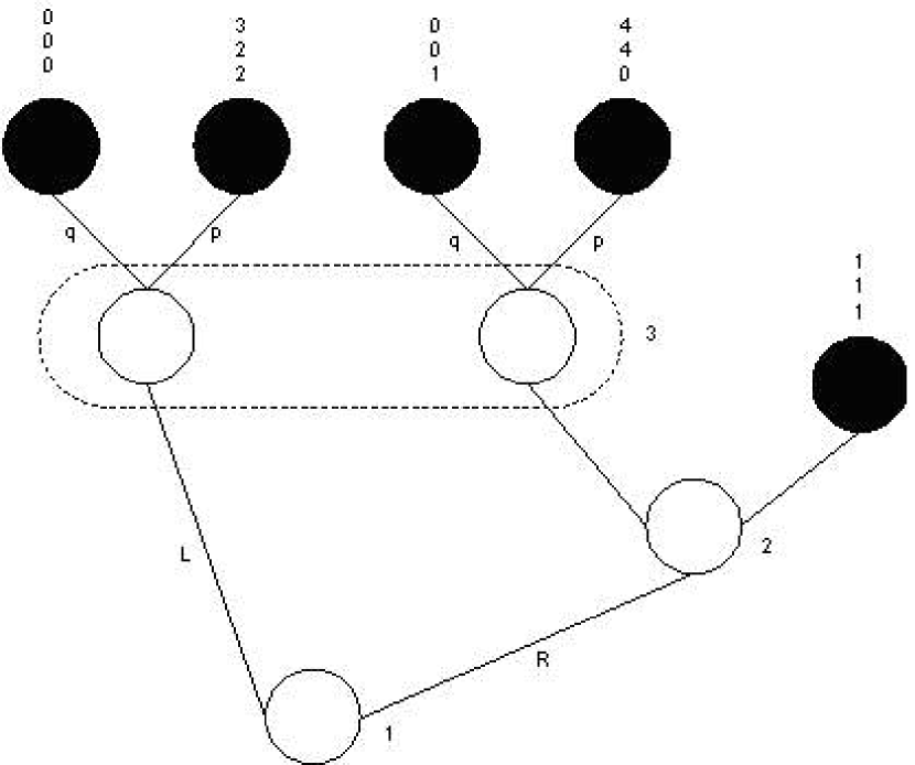
Figure 4.1: Selten’s Horse Game Tree

This game possesses both a perfect equilibrium as well as “non-sensical” subgame perfect equilibria. The perfect equilibrium for this extensive form game is defined via the perturbed pay-off functions:

$$R_{1} = \alpha_{1}(1-\varepsilon_{2}-3\varepsilon_{3}+4\varepsilon_{2}\varepsilon_{3})+3\varepsilon_{3}$$

$$R_{2} = 2\varepsilon_{3}(2-\varepsilon_{1})+\alpha_{2}(1-\varepsilon_{1}-4e_{3}+4\varepsilon_{1}\varepsilon_{3})$$

$$R_{3} = 1-\varepsilon_{1}+\alpha_{3}(2\varepsilon_{1}-\varepsilon_{2}+\varepsilon_{1}\varepsilon_{2}),$$

where the $\alpha_{i}$ are the mixed strategies and $\varepsilon_{i}$ are errors defined for $i=1,2,3$. Letting the errors approach zero, it can be seen that perfect equilibrium is defined by $\left(1,1,0\right)$.

The results of the simulation are shown below in Figure 4.2 and indicate convergence to the trembling hand perfect equilibrium.

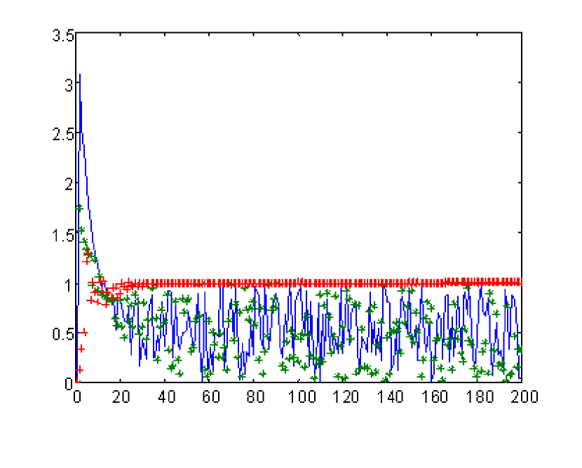
Figure 4.2: Three-person game with imperfect competition and payoff solutions

5 Conclusion

This paper has concentrated on some of the underlying theoretical mechanics of simulated annealing and how they relate to the trembling hand perfect refinement of Nash equilibrium. It has been argued that the trembles that underlie global optimization by simulated annealing are analogous to the “mistakes” of trembling hand perfection, in that they present a means of moving from local equilibria. The main contribution of this paper has been to apply simulated annealing to solve a game that is known to possess both a perfect equilibrium and “nonsensical” subgame perfect equilibrium. Preliminary results indicate a convergence to the perfect equilibrium, with a mixing strategy occurring for two of the three players.

References

- [1] Besag, J. (1974) Spatial interaction and the statistical analysis of lattice systems (with discussion). Journal of the Royal Statistical Society Series B 36, 192–236.
- [2] Friedman, J.W. (1991) Game Theory with Applications to Economics. Oxford University Press, Oxford.
- [3] Georgobiani, D. A. and Torondzadze, A. F (1980) Solution of rectangular games by the Monte Carlo method. Trudy Vychisl. Tsentra Akad. Nauk Gruzin. SSR 20(2), 5–10.
- [4] Gilks, W.R., Richardson, S. Spiegelhalter, D.J. (1996) Introducing Markov Chain Monte Carlo. In Gilks, W.R., Richardson, S. Spiegelhalter, D.J. (Eds..) Markov Chain Monte Carlo in Practice, 1–19. Chapman and Hall, London.
- [5] Gilks, W.R. (1996) Full conditional distributions. In Gilks, W.R., Richardson, S. Spiegelhalter, D.J. (Eds.) Markov Chain Monte Carlo in Practice, 75–88. Chapman and Hall, London.
- [6] Harsanyi, J.C., (1975) The tracing procedure: a Bayesian approach to defining a solution for -person non-cooperative games. International Journal of Game Theory 4, 1-22.
- [7] Harsanyi, J.C. and Selten, R. (1988) A General Theory of Equilibrium Selection in Games. MIT Press, Cambridge, MA.
- [8] Hastings, W.K. (1970) Monte Carlo sampling methods using Markov chains and their application. Biometrika 57, 97–109.
- [9] Kuhn, H.W. (1953) Extensive games and the problem of information. In Kuhn, H.W. and Tucker, A.W. Contributions to the Theory of Games Vol I, 193–216. Princeton University Press, Princeton N.J.
- [10] Lempke, C.E. and Howson, J.T. (1964) Equilibrium points of bimatrix games. SIAM Journal on Applied Mathematics 12, 413–423.
- [11] Metropolis, N., Rosenbluth, A.W., Rosenbluth, M.N., Teller, A.H., Teller, E., (1953) Equations of state calculations by fast computing machines. Journal of Chemistry Physics 21, 1087–1091.
- [12] Myerson, R.B. (1978) Refinements of the concept of Nash equilibrium. International Journal of Game Theory 7, 73–80.
- [13] Myerson, R.B. (1991) Game Theory: Analysis of Conflict. Harvard University Press, Cambridge, MA.
- [14] Roberts, G.O. (1996) Markov chain concepts related to sampling algorithms. In Gilks, W.R., Richardson, S. Spiegelhalter, D.J. (Eds.) Markov Chain Monte Carlo in Practice, 45–57. Chapman and Hall, London.
- [15] Scarf, H.E. (1973) Computation of Economic Equilibria. Yale University Press, New Haven, Conn.
- [16] Selten, R. (1975) Reexamination of the Perfectness Concept for Equilibrium Concepts in Extensive Form Games. International Journal of Game Theory 4, 25–55.
- [17] Selten, R. (1978) The Chain Store Paradox. Theory and Decision 9, 127–159.
- [18] Ulam, S. (1954) Applications of Monte Carlo methods to tactical games. In Meyer, H.A. (Ed.) Symposium on Monte Carlo Methods, University of Florida 1954, p. 63. John Wiley and Sons, New York.
- [19] van Damme, E. (1991) Stability and Perfection of Nash Equilibria (2nd ed. rev. enl.). Springer-Verlag, Berlin.
- [20] van Laarhoven, P.J.M. and Aarts, E.H.L. (1987) Simulated Annealing: Theory and Applications. D. Reidel Publishing, Dordrecht, Holland.
- [21] Wilson, R. (1971) Computing Equilibria of -Person Games. SIAM Journal on Applied Mathematics 21, 80–87.