Optimal Covering Tours with Turn Costs

Abstract

We give the first algorithmic study of a class of “covering tour” problems related to the geometric Traveling Salesman Problem: Find a polygonal tour for a cutter so that it sweeps out a specified region (“pocket”), in order to minimize a cost that depends mainly on the number of turns. These problems arise naturally in manufacturing applications of computational geometry to automatic tool path generation and automatic inspection systems, as well as arc routing (“postman”) problems with turn penalties. We prove the NP-completeness of minimum-turn milling and give efficient approximation algorithms for several natural versions of the problem, including a polynomial-time approximation scheme based on a novel adaptation of the $m$-guillotine method.

1 Introduction

An important algorithmic problem in manufacturing is to compute effective paths and tours for covering (“milling”) a given region (“pocket”) with a cutting tool. The objective is to find a path or tour along which to move a prescribed cutter in order that the sweep of the cutter covers the region, removing all of the material from the pocket, while not “gouging” the material that lies outside of the pocket. This covering tour or “lawn mowing” problem [6] and its variants arise not only in NC machining applications but also in automatic inspection, spray painting/coating operations, robotic exploration, arc routing, and even mathematical origami.

The majority of research on these geometric covering tour problems as well as on the underlying arc routing problems in networks has focused on cost functions based on the lengths of edges. However, in many actual routing problems, this cost is dominated by the cost of switching paths or direction at a junction. A drastic example is given by fiber-optical networks, where the time to follow an edge is negligible compared to the cost of changing to a different frequency at a router. In the context of NC machining, turns represent an important component of the objective function, as the cutter may have to be slowed in anticipation of a turn. The number of turns (“link distance”) also arises naturally as an objective function in robotic exploration (minimum-link watchman tours) and in various arc routing problems, such as snow plowing or street sweeping with turn penalties. R. Klein [35] has posed the question of minimizing the number of turns in polygon exploration problems.

In this paper, we address the problem of minimizing the cost of turns in a covering tour. This important aspect of the problem has been left unexplored so far in the algorithmic community, and the arc routing community has examined only heuristics without performance guarantee, or exact algorithms with exponential running time. Thus, our study provides important new insights and a better understanding of the problems arising from turn cost. We present several new results:

1. We prove that the covering tour problem with turn costs is NP-complete, even if the objective is purely to minimize the number of turns, the pocket is orthogonal (rectilinear), and the cutter must move axis-parallel. The hardness of the problem is not apparent, as our problem seemingly bears a close resemblance to the polynomially solvable Chinese Postman Problem; see the discussion below.

2. We provide a variety of constant-factor approximation algorithms that efficiently compute covering tours that are nearly optimal with respect to turn costs in various versions of the problem. While getting some $O(1)$-approximation is not difficult for most problems in this class, through a careful study of the structure of the problem, we have developed tools and techniques that enable significantly stronger approximation results.

   One of our main results is a 3.75-approximation for minimum-turn axis-parallel tours for a unit square cutter that covers an integral orthogonal polygon, possibly with holes. Another main result gives a 4/3-approximation for minimum-turn tours in a “thin” pocket, as arises in the arc routing version of our problem.

   Table 1 summarizes our results. The term “coverage” indicates the number of times a point is visited, which is of interest in several practical applications. This parameter also provides an upper bound on the total length.

3. We devise a polynomial-time approximation scheme (PTAS) for the covering tour problem in which the cost is given as a weighted combination of length and number of turns, i.e., the Euclidean length plus a constant $C$ times the number of turns. For an integral orthogonal polygon with $h$ holes and $N$ pixels, the running time is $2^{O(h)}\cdot N^{O(C)}$. The PTAS involves an extension of the $m$-guillotine method, which has previously been applied to obtain PTAS’s in problems involving only length [38].

We should stress that our paper focuses on the graph-theoretic and algorithmic aspects of the turn-cost problem; we make no claims of immediate applicability of our methods for NC machining.

Discrete Thin Orthogonal Thin Milling Discrete Milling Orthogonal Section 5.1.1 5.1.2 5.3 5.4 Cycle cover APX $2{\delta}+{\rho}$ 4 1.5 4.5 1 Tour APX $2{\delta}+{\rho}+2$ 6 3.5 6.25 4/3 Length APX ${\delta}$ 2 - 8 4 Max cover ${\delta}$ $2{\rho}$ - 8 4 Time (explicit) $O(N)$ $O(N)$ $O(N^{3})$ $O(N^{2.376}+n^{3})$ $O(n^{3})$ Time (implicit) n/a n/a n/a $O(n^{2.5}\log N+n^{3})$ $O(n^{3})$

Integral Orthogonal Section 5.2 Cycle cover APX 10 4 2.5 Tour APX 12 6 3.75 Length APX 4 4 4 Max cover 4 4 4 Time (explicit) $O(N)$ $O(N^{2.376})$ $O(N^{2.376}+n^{3})$ Time (implicit) $O(n\log n)$ $O(n^{2.5}\log N)$ $O(n^{2.5}\log N+n^{3})$

Table 1: Approximation factors achieved by our (polynomial-time) algorithms. Rows marked “APX” give approximation factors for the minimum-turn cycle cover (“Cycle cover”), the minimum-turn covering tour (“Tour”), and the simultaneous approximation of length of a covering tour (“Length”). The row marked “Max Cover” indicates the maximum number of times a point is visited. The parameter ${\delta}$ denotes the maximum degree in the underlying graph, while the parameter ${\rho}$ is the maximum number of directions in the graph. The two rows for running time refer to an “explicit” description of input pixels and output and a more compact “implicit” encoding of pixels and output. (See Section 2 for more detailed definitions.)

Related Work

In the CAD community, there is a vast literature on the subject of automatic tool-path generation; we refer the reader to Held [27] for a survey and for applications of computational geometry to the problem. The algorithmic study of the problem has focused on the problem of minimizing the length of a milling tour: Arkin, Fekete, and Mitchell [5, 6] show that the problem is NP-hard for the case where the mower is a square. Constant-factor approximation algorithms are given in [5, 6, 30], with the current best factor being a 2.5-approximation for min-length milling (11/5-approximation for orthogonal simple polygons). For the closely related lawn mowing problem (also known as the “traveling cameraman problem” [30]), in which the covering tour is not constrained to stay within $P$, the best current approximation factor is $3+\varepsilon$ (utilizing PTAS results for TSP). Also closely related is the watchman route problem with limited visibility (or “$d$-sweeper problem”); Ntafos [42] provides a 4/3-approximation, and Arkin, Fekete, and Mitchell [6] improve this factor to 6/5. The problem is also closely related to the Hamiltonicity problem in grid graphs; the results of [44] suggest that in simple polygons, minimum-length milling may in fact have a polynomial-time algorithm.

Covering tour problems are related to watchman route problems in polygons, which have received considerable attention in terms of both exact algorithms (for the simple polygon case) and approximation algorithms (in general); see [39] for a relatively recent survey. Most relevant to our problem is the prior work on minimum-link watchman tours: see [2, 3, 8] for hardness and approximation results, and [14, 36] for combinatorial bounds. However, in these problems the watchman is assumed to see arbitrarily far, making them distinct from our tour cover problems.

Other algorithmic results on milling include a study of multiple tool milling by Arya, Cheng, and Mount [9], which gives an approximation algorithm for minimum-length tours that use different size cutters, and the paper of Arkin, Held, and Smith [7], which examines the problem of minimizing the number of retractions for “zig-zag” machining without “re-milling”, showing that the problem is NP-complete and giving an $O(1)$-approximation algorithm.

Geometric tour problems with turn costs have been studied by Aggarwal et al. [1], who study the angular-metric TSP. The objective is to compute a tour on a set of points, such that the sum of the direction changes at vertices is minimized: For any vertex $v_{i}$ with incoming edge $v_{i-1}v_{i}$ and outgoing edge $v_{i}v_{i+1}$, the change of direction is given by the absolute value of the angle between $v_{i-1}v_{i}$ and $v_{i}v_{i+1}$. The problem turns out to be NP-hard, and an $O(\log n)$ approximation is given. Fekete [20] and Fekete and Woeginger [21] have studied a variety of angle-restricted tour (ART) problems. Covering problems of a different nature have been studied by Demaine et al. [16], who considered algorithmic issues of origami.

In the operations research literature, there has been an extensive study of arc routing problems, which arise in snow removal, street cleaning, road gritting, trash collection, meter reading, mail delivery, etc.; see the surveys of [10, 18, 19]. Arc routing with turn costs has had considerable attention, as it enables a more accurate modeling of the true routing costs in many situations. Most recently, Clossey, Laporte, and Soriano [13] present six heuristic methods of attacking arc routing with turn penalties, without resorting to the usual transformation to a TSP problem; however, their results are purely based on experiments and provide no provable performance guarantees. The directed postman problem in graphs with turn penalties has been studied by Benavent and Soler [11], who prove the problem to be (strongly) NP-hard and provide heuristics (without performance guarantees) and computational results. (See also Fernández’s thesis [22] and [41] for computational experience with worst-case exponential-time exact methods.)

Our covering tour problem is related to the Chinese Postman Problem (CPP), which can be solved exactly in polynomial time for “purely” undirected or purely directed graphs. However, the turn-weighted CPP is readily seen to be NP-complete: Hamiltonian cycle in line graphs is NP-complete (contrary to what is reported in [25]; see page 246 of West [45]), implying that TSP in line graphs is also NP-complete. The CPP on graph $G$ with turn costs at nodes (and zero costs on edges) is equivalent to TSP on the corresponding line graph, ${\cal L}(G)$, where the cost of an edge in ${\cal L}(G)$ is given by the corresponding turn cost in $G$. Thus, the turn-weighted CPP is also NP-complete.

2 Preliminaries

This section formally defines the problems at hand, and various special cases of interest.

Problem Definitions

The general geometric milling problem is to find a closed curve (not necessarily simple) whose Minkowski sum with a given tool (cutter) is precisely a given region $P$ bounded by $n$ edges. In the context of numerically controlled (NC) machines, this region is usually called a pocket. Subject to this constraint, we may wish to optimize a variety of objective functions, such as the length of the tour, or the number of turns in the tour. We call these problems minimum-length and minimum-turn milling, respectively. While the latter problem is the main focus of this paper, we are also interested in bicriteria versions of the problem in which both length and number of turns must be small; we also consider the scenario in which the objective function is given by a linear combination of turn cost and distance traveled (see Section 5.5).

In addition to choices in the objective function, the problem version depends on the constraints on the tour. The most general case arises when considering a tour that has to visit a discrete set of vertices, connected by a set of edges, with a specified turn cost at each vertex to change from one edge to the next. More precisely, at each vertex, the tour has the choice of (0) going “straight”, if there is one “collinear” edge with the one currently used (costing no turn), (1) turning onto another, non-collinear edge (costing one turn), or (2) “U-turning” back onto the source edge (costing two turns). Which pairs of the $d$ edges incident to a degree-$d$ vertex are considered “collinear” is specified by a matching in the complete graph $K_{d}$: three incident edges cannot be “collinear”. We call this graph-theoretic abstraction the discrete milling problem, indicating the close relationship to other graph-theoretic tour optimization problem. We are able to give a number of approximation algorithms for discrete milling that depend on some graph parameters: ${\delta}$ denotes the maximum degree of a vertex and ${\rho}$ denotes the maximum number of distinct “directions” coming together at a vertex. (For example, for graphs arising from $d$-dimensional grids, these values are bounded by $2d$ and $d$, respectively.)

A special case of discrete milling arises when dealing with “thin” structures in two- or three-dimensional space, where the task is to travel all of a given set of “channels”, which are connected at vertices. This resembles a CPP, in that it requires us to travel a given set of edges; however, in addition to the edge cost, there is a cost at the vertices when moving from one edge to the next. For this scenario, we are able to describe approximation factors that are independent of other graph parameters.

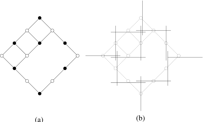
More geometric problems arise when considering the milling of a polygonal region $P$. In the orthogonal milling problem, the region $P$ is an orthogonal polygonal domain (with holes) and the tool is an (axis-parallel) unit-square cutter constrained to axis-parallel motion, with edges of the tour alternating between horizontal and vertical. All turns are orthogonal; $90^{\circ}$ turns incur a cost of 1, while a “U-turn” has a cost of 2. In the integral orthogonal case, all coordinates of boundary edges are integers, so the region can be considered to be the (connected) union of $N$ pixels, i.e., axis-parallel unit squares with integer vertices. Note that in general, $N$ may not be bounded by a polynomial in $n$. Instead of dealing directly with a geometric milling problem, we often find it helpful to consider a more combinatorial problem, and then adapt the solution back to the geometric problem. In particular, for integral orthogonal milling, we may assume that an optimal tour can be assumed to have its vertex coordinates of the form $k+\frac{1}{2}$ for integral $k$. Then, milling in an integral orthogonal polygon (with holes) is equivalent to finding a tour of all the vertices (“pixels”) of a grid graph; see Figure 1.

Figure 1: An instance of the integral orthogonal milling problem (left) and the grid graph model (right).

An interesting special case of integral orthogonal milling is the thin orthogonal milling problem, in which the region does not contain a 2$\times$2 square of pixels. This is also closely related to discrete milling, as we can think of edges embedded into the planar grid, such that vertices and channels are well separated. This problem of finding a tour with minimum turn cost for this class of graphs is still NP-complete, even for a subclass for which the corresponding problem of minimizing total distance is trivial; this highlights the particular difficulty of dealing with turn cost. On the other hand, thin orthogonal milling allows for particularly fast and efficient approximation algorithms.

Other Issues

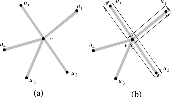
It should be stressed that using turn cost instead of (or in addition to) edge length changes several characteristics of distances. One fundamental problem is illustrated by the example in Figure 2: the triangle inequality does not have to hold when using turn cost. This implies that many classical algorithmic approaches for graphs with nonnegative edge weights (such as using optimal 2-factors or the Christofides method for the TSP) cannot be applied without developing additional tools.

Figure 2: The triangle inequality may not hold when using turn cost as distance measure: $d(a,c)=3>2=d(a,b)+d(b,c)$

In fact, in the presence of turn costs we distinguish between the terms 2-factor, i.e., a set of edges, such that every vertex is incident to two of them, and cycle cover, i.e., a set of cycles, such that every vertex is covered. While the terms are interchangeable when referring to the set of edges that they constitute, we make a distinction between their respective costs: a “2-factor” has a cost consisting of the sum of edge costs, but does not necessarily account for the turn cost between it two incident edges, while the cost of a “cycle cover” includes also the turn costs at vertices.

It is often useful in designing approximation algorithms for optimal tours to begin with the problem of computing an optimal cycle cover, minimizing the total number of turns in a set of cycles that covers $P$. Specifically, we can decompose the problem of finding an optimal (minimum-turn) tour into two tasks: finding an optimal cycle cover, and merging the components. Of course, these two processes may influence each other: there may be several optimal cycle covers, some of which are easier to merge than others. (In particular, we say that a cycle cover is connected, if the graph induced by the set of cycles and their intersections is connected.) As we will show, even the problem of optimally merging a connected cycle cover is NP-complete. This is in contrast to minimum-length milling, where an optimal connected cycle cover can trivially be converted into an optimal tour that has the same cost.

Algorithms whose running time is polynomial in the explicit encoding size (pixel count) are pseudo-polynomial. Algorithms whose running time is polynomial in the implicit encoding size are polynomial. This distinction becomes an important issue when considering different ways to encode input and output; e.g., a large set of pixels forming an $a\times b$ rectangle can be described in space $O(\log a+\log b)$ by simply describing the bounding edges, instead of listing all $ab$ individual pixels. In integral orthogonal milling, one might think that it is most natural to encode the grid graph with vertices, because the tour will be embedded on this graph and will, in general, have complexity proportional to the number $N$ of pixels. But the input to any geometric milling problem has a natural encoding by specifying only the $n$ vertices of the polygon $P$. In particular, long edges are encoded in binary (or with one real number, depending on the model) instead of unary. It is possible to get a running time depending only on this size, but of course we need to allow for the output to be encoded implicitly. That is, we cannot explicitly encode each vertex of the tour, because there are too many (the number can be arbitrarily large even for a succinctly encodable rectangle). Instead, we encode an abstract description of the tour that is easily decoded.

Finally, we mention that many of our results carry over from the tour (or cycle) version to the path version, in which the cutter need not return to its original position. In this paper, we omit the straightforward changes necessary to compute optimal paths. A similar adjustment can be made for the related case of lawn mowing, in which the sweep of the cutter is allowed to go outside $P$ during its motion. Clearly, our techniques are also useful for scenarios of this type.

3 NP-Completeness

Arkin, Fekete, and Mitchell [6] have proved that the problem of optimizing the length of a milling tour is NP-hard. Their proof is based on the well-known hardness of deciding whether a grid graph has a Hamiltonian cycle [29, 31]. This result implies that it is NP-hard to find a tour of minimum total length that visits all vertices. If, on the other hand, we are given a connected cycle cover of a graph that has minimum total length, then it is trivial to convert it into a tour of the same length by merging the cycles into one tour.

In this section we show that if the quality of a tour is measured by counting turns, then even this last step of turning an optimal connected cycle cover into an optimal tour is NP-complete. Thus we prove that it is NP-hard to find a milling tour that optimizes the number of turns for a polygon with holes.

Theorem 1.

Minimum-turn milling is NP-complete, even when we are restricted to the orthogonal thin case, and are already provided with an optimal connected cycle cover.

Because thin orthogonal milling is a special case of thin milling as well as orthogonal milling, and it is easy to convert an instance of thin orthogonal milling into an instance of integral orthogonal milling, we have

Corollary 2.

Discrete milling, orthogonal milling, and integral orthogonal milling are NP-complete.

Theorem 1.

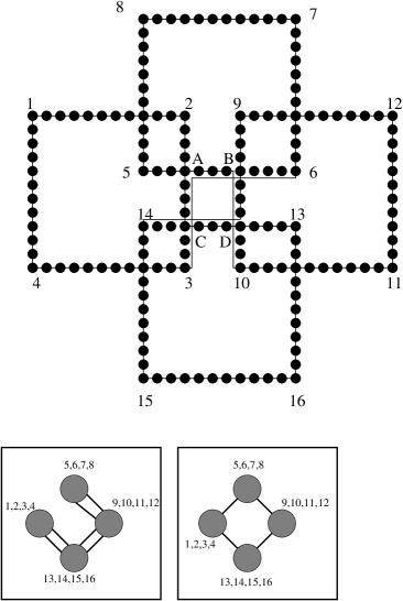
Our reduction proceeds in two steps. First we show that the problem Hamiltonicity of Unit Segment Intersection Graphs (Husig) of deciding the Hamiltonicity of intersection graphs of axis-parallel unit segments is hard. To see this, we use the NP-hardness of deciding Hamiltonicity of grid graphs ([29, 31]) and argue that any grid graph can be represented in this form; see Figure 3:

Figure 3: (a) A grid graph $G$. (b) A representation of $G$ as an intersection graph of axis-parallel unit segments.

Consider a set of integer grid points that induce a grid graph $G$. Note that $G$ is bipartite, because one can 2-color the nodes by coloring a grid point $(x,y)$ black (resp., white) if $x+y$ is odd (resp., even). After rotating the point set by $\pi/4$, the coordinate of each point is an integer multiple of $1/\sqrt{2}$. Scaling down the resulting arrangement by a factor of $3/\sqrt{2}$ results in an arrangement in which the coordinate of each point is an integer multiple of $1/3$, and the shortest distance between two points of the same color class is $2/3$. For the resulting set of points $p_{i}=(x_{i},y_{i})$, let $p^{\prime}_{i}=p_{i}+(\varepsilon_{i},\varepsilon_{i})$ be given as the set obtained by “perturbations” $\varepsilon_{i}$ that are small and all distinct. Then, represent each “white” vertex by a horizontal unit segment centered at $p^{\prime}_{i}$, and each “black” vertex by a vertical unit segment centered at $p^{\prime}_{i}$. Now it is easy to see that the resulting unit segment intersection graph is precisely the original grid graph $G$.

In a second step, we show that the problem Husig reduces to the problem of milling with turn costs. The outline of our argument is illustrated in Figure 4.

Figure 4: Thin orthogonal milling with turn cost is NP-hard: (a) a set of $s=8$ axis-parallel unit segments, denoted by $s_{1},\ldots,s_{8}$; (b) the corresponding intersection graph $G$, with the Hamiltonian cycle $v_{1},v_{2},v_{3},v_{6},v_{7},v_{8},v_{5},v_{4}$ shown in bold; (c) representing $G$ by a connected region consisting of $4s$ corridors; (d) a drawing of the graph induced by the instance of thin orthogonal milling, with the $s=8$ rectangular cycles $C_{1},\ldots,C_{8}$; (e) a milling tour with $5s$ turns corresponding to the Hamiltonian cycle in $G$; (f) milling the four corridors of a cycle using five turns.

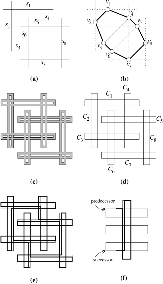
Consider a unit segment intersection graph $G$, given by a set of axis-parallel unit segments, as shown in Figure 4(a). Figure 4(b) shows the corresponding graph, with a Hamiltonian cycle indicated in bold. Without loss of generality, we may assume that $G$ is connected. Let $s$ be the number of nodes of $G$.

As shown in Figure 4(c), we replace each line segment by a cycle of four thin axis-parallel corridors. This results in a connected polygonal region $P$ having $4s$ convex corners. Clearly, any cycle cover or tour cover of $P$ must have at least $4s$ turns; by using a cycle for each set of four corridors representing a strip, we get a cycle cover $\cal C$ with $4s$ turns. Therefore, $\cal C$ is an optimal cycle cover, and it is connected, because $G$ is connected.

Now assume that $G$ has a Hamiltonian cycle. It is easy to see (Figure 4(f)) that this cycle can be used to construct a milling tour of $P$ with a total of $5s$ turns: Each time the Hamiltonian cycle moves from one vertex $v_{i}$ of the grid graph to the next vertex $v_{j}$, the milling tour moves from the cycle $C_{i}$ representing $v_{i}$ to the cycle $C_{j}$ representing $v_{j}$, at an additional cost of 1 turn for each of the $s$ edges in the Hamiltonian cycle.

Assume conversely that there is a milling tour $T$ with at most $5s$ turns. We refer to turns at the corners of 4-cycles as convex turns. The other turns are called crossing turns.

As noted above, the convex corners of $P$ require at least $4s$ convex turns. Consider the sequence of turns $t_{1},\ldots,t_{5s}$ in $T$. By construction, the longest contiguous subsequence of convex turns contains at most four different convex turns. (More precisely, we can only have such a subsequence with four different convex corners, if these four corners belong to the same 4-cycle representing a unit segment.) Furthermore, we need at least one additional crossing turn at an interior crossing of two corridors to get from one convex corner to another convex corner not on the same 4-cycle. (More precisely, one crossing turn is sufficient only if the two connected convex corners belong to 4-cycles representing intersecting unit segments.) Therefore, we need at least $c$ crossing turns if we have at least $c$ contiguous subsequences as described above. This means that $c\geq s$; hence, $c=s$ by the assumption on the number of turns on $T$. Because the $c$ crossing turns correspond to a closed roundtrip in $G$ that visits all $s$ vertices, this implies that we have a Hamiltonian cycle, concluding the proof. ∎

4 Approximation Tools

There are three main tools that we use to develop approximation algorithms: computing optimal cycle covers for milling the “boundary” of $P$ (Section 4.1), converting cycle covers into tours (Section 4.2), and using optimal (or nearly-optimal) “strip covers” (Section 4.3). In this section, our description mostly focuses on orthogonal milling; however, we will see in the following Section 5.1 how some of our tools can also be applied to the general case of discrete milling.

4.1 Boundary Cycle Covers

We consider first the problem of finding a minimum-turn cycle cover for covering a certain subset, $\overline{P}$, of $P$ that is along its boundary. This will turn out to be a useful tool for approximation algorithms. Specifically, in orthogonal milling we define the set $\overline{P}$ of boundary pixels to consist of pixels that have at least one of their four edges on a boundary edge of the polygon; i.e., in the grid graph that describes adjacency of pixels, these are pixels of degree at most 3. Let $N_{\overline{P}}$ be the number of boundary pixels. A boundary cycle cover is a collection of cycles that visit all boundary pixels.

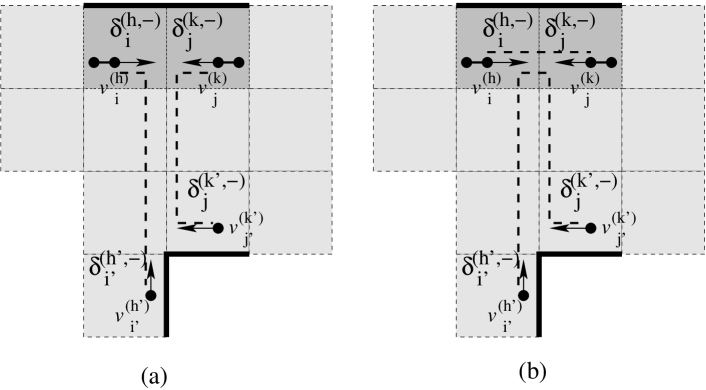
We define an auxiliary structure, $G_{\overline{P}}=(V_{\overline{P}},E_{\overline{P}})$, which is a complete weighted graph on $2N_{\overline{P}}$ vertices; for ease of description, we will refer to $G_{\overline{P}}$ as a set of points and paths between them. This will allow us to map boundary cycle covers in $P$ to matchings of corresponding turn cost in $G_{\overline{P}}$. For this purpose, map each pixel $p_{i}\in\overline{P}$ to two vertices in $V_{\overline{P}}$, $v_{i}^{(0)}$ and $v_{i}^{(1)}$. For each boundary pixel $p_{i}$, this pair represents an orientation that is attained by a cutter when visiting $p_{i}$. Depending on the boundary structure of $p_{i}$, there are four different cases; refer to Figure 5.

Figure 5: Representing a boundary pixel $p_{i}$ by a pair of vertices $v_{i}^{(0)}$ and $v_{i}^{(1)}$.

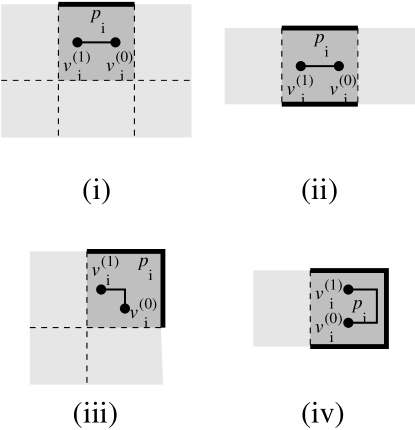
(i) One edge of $p_{i}$ is a boundary edge of the polygon.

(ii) Two opposite edges of $p_{i}$ are boundary edges of the polygon.

(iii) Two adjacent edges of $p_{i}$ are boundary edges of the polygon.

(iv) Three edges of $P_{i}$ are boundary edges of the polygon.

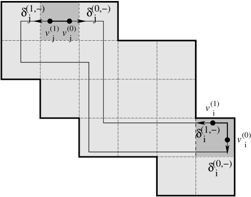
For easier description, we refer to the vertices $v_{i}^{(0)}$ and $v_{i}^{(1)}$ as points embedded within $p_{i}$, as shown in Figure 5. Furthermore, we add a mandatory path $m_{i}$ between $v_{i}^{(0)}$ and $v_{i}^{(1)}$, represented by a polygonal path with $c(m_{i})=0$ (cases (i) and (ii)), $c(m_{i})=1$ (case (iii)) or $c(m_{i})=2$ turns (case (iv)), as shown in the figure. This path maps the contour of $P$ at $p_{i}$, and it represents orientations that a cutter has to attain when visiting pixel $p_{i}$. Note that traveling from $v_{i}^{(h)}$ to $v_{j}^{(1-h)}$ along $m_{i}$ induces a heading $\delta_{i}^{(h,-)}$ when leaving $v_{i}^{(h)}$ and a heading $\delta_{i}^{(1-h,+)}$ when arriving at $v_{i}^{(1-h)}$. Note that $\delta_{i}^{(h,-)}$ is opposite to $\delta_{i}^{(h,+)}$.

Now we add a set of optional paths, representing the weighted edges $E_{\overline{P}}$ of the complete graph $G_{\overline{P}}$. For an example, refer to Figure 6. For any pair of vertices $v_{i}^{(h)}$ and $v_{j}^{(k)}$, let $d(v_{i}^{(h)},v_{j}^{(k)})$ be the minimum number of turns necessary when traveling from $v_{i}^{(h)}$ with heading $\delta_{i}^{(h,+)}$ to $v_{j}^{(k)}$ with heading $\delta_{j}^{(k,-)}$. Note that $d(v_{i}^{(h)},v_{j}^{(k)})=d(v_{j}^{(k)},v_{i}^{(h)})$, as any shortest path can be traveled in the opposite direction. Using a Dijkstra-like approach, we can compute these distances from one boundary pixel to all other boundary pixels in time $O(N_{\overline{P}}\log N_{\overline{P}})$; see the overview in [39] or the paper [37]. The overall time of $O(N_{\overline{P}}^{2}\log N_{\overline{P}})$ for computing all these link distances is dominated by the following step: In time $O(N_{\overline{P}}^{3})$ [24, 43], find a minimum-weight perfect matching in the complete weighted graph $G_{\overline{P}}$.

Figure 6: The cost of traveling between two pixels: $d(v_{i}^{(1)},v_{j}^{(0)})=d(v_{j}^{(0)},v_{i}^{(1)})=2$, while $d(v_{i}^{(0)},v_{j}^{(1)})=d(v_{j}^{(1)},v_{i}^{(0)})=5$.

Now it is not hard to see the following.

Lemma 3.

Any boundary cycle cover in $P$ with $t$ turns can be mapped to a perfect matching in $G_{\overline{P}}$ of cost $t-\sum_{p_{i}\in\overline{P}}c(m_{i})$, and vice versa.

Proof.

Whenever a boundary cycle cover visits a boundary pixel $p_{i}$, it has to perform the turns corresponding to the mandatory path $m_{i}$. Moreover, moving from one pixel $p_{i}$ to the next pixel $p_{j}$ can be mapped to the optional path corresponding to the edges $(v_{i}^{(h)},v_{j}^{(k)})$; clearly, the overall cost is as stated.

Conversely, it is straightforward to see that the combination of a perfect matching in $G_{\overline{P}}$ and the mandatory paths yields a boundary cycle cover of corresponding cost. ∎

Using the algorithms described above, we also obtain the following:

Theorem 4.

Given the set of $N_{\overline{P}}$ boundary pixels, a minimum-turn boundary cycle cover can be computed in time $O(N_{\overline{P}}^{3})$, the time it takes to compute a perfect matching in $G_{\overline{P}}$.

If the set of pixels is not given in unary, but implicitly as the pixels contained in a region with $n$ edges, the above complexity is insufficient. However, we can use local modifications to argue the following tool for speeding up the search for an optimal perfect matching.

Lemma 5.

Let $p_{i}$ and $p_{j}$ be neighboring boundary pixels that are adjacent to the same boundary edge, so $d(v_{i}^{(h)},v_{j}^{(k)})=0$ for an appropriate choice of $h$ and $k$. Then there is an optimal matching containing $(v_{i}^{(h)},v_{j}^{(k)})$.

Proof.

This follows by a simple exchange argument. See Figure 7. Suppose two adjacent pixels $p_{i}$ and $p_{j}$ along the same boundary edge are not matched to each other, let $v_{i}^{(h)}$ be the vertex such that $\delta_{i}(h,-)$ is heading for $p_{j}$, and let $v_{j}^{(k)}$ be the vertex such that $\delta_{j}(k,-)$ is heading for $p_{i}$. Furthermore suppose that $v_{i^{\prime}}^{(h^{\prime})}$ is matched to $v_{i}^{(h)}$ and $v_{j^{\prime}}^{(k^{\prime})}$ is matched to $v_{j}^{(k)}$. Then we can match $v_{i^{\prime}}^{(h^{\prime})}$ to $v_{j^{\prime}}^{(k^{\prime})}$ and $v_{i}^{(h)}$ to $v_{j}^{(k)}$ without changing the cost of the matching. ∎

Figure 7: By performing local modifications, an optimal cycle cover can be assumed to cover each collinear piece of the boundary in one connected strip.

This allows us to obtain a strongly polynomial version of the matching algorithm of Theorem 4.

Theorem 6.

A minimum-turn boundary cycle cover can be computed in time $O(n^{3})$.

Proof.

By applying Lemma 5 repeatedly, we get $O(n)$ connected boundary strips, consisting of sets of collinear boundary pixels. These can be determined efficiently by computing offsets of the boundary edges. This leaves only $O(n)$ endpoints of such strips to be matched, resulting in the claimed complexity. ∎

Note that the validity of this argument is not restricted to the integral orthogonal case, but remains valid even for orthogonal regions with arbitrary boundary edges.

Remark

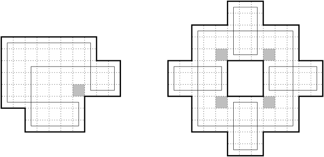
The definition of the “boundary” pixels $\overline{P}$ used here does not include all pixels that touch the boundary of $P$ in a diagonal fashion; in particular, it omits the “reflex pixels” that share a corner, but no edge, with the boundary of $P$. It seems difficult to require that the cycle cover mill reflex pixels, because Lemma 5 does not extend to this case, and an optimal cycle cover of the boundary (as defined above) may have fewer turns than an optimal cycle cover that mills the boundary $\overline{P}$ plus the reflex pixels; see Figure 8.

Figure 8: Optimally covering all pixels that have an edge against the boundary can leave reflex pixels uncovered.

4.2 Merging Cycles

It is often easier to find a minimum-turn cycle cover (or constant-factor approximation thereof) than to find a minimum-turn tour. We show that an exact or approximate minimum-turn cycle cover implies an approximation for a minimum-turn tour.

We concentrate on the integral orthogonal case. First we define a few terms precisely. Two pixels are adjacent if the distance between their centers is $1$. Two cycles $T_{1}$, $T_{2}$ are intersecting iff $T_{1}\cap T_{2}\neq\emptyset$. Two cycles are called touching if and only if they are not intersecting and there exist pixels $p_{1}\in T_{1}$, $p_{2}\in T_{2}$ such that $p_{1}$ and $p_{2}$ are adjacent.

Lemma 7.

Let $P_{1}$ and $P_{2}$ be two cycles, with $t_{1}$ and $t_{2}$ turns, respectively, and let $p$ be a pixel that is contained in both cycles. Then there is a cycle milling the union of pixels milled by $P_{1}$ and $P_{2}$ and having at most $t_{1}+t_{2}+2$ turns. This cycle can be found in time linear in the number of its turns.

Proof.

Let the neighbors of $p$ in $P_{1}$ be $a_{1}$, $a_{2}$ and those of $p$ in $P_{2}$ be $b_{1}$, $b_{2}$. Connect $a_{1}$ via $p$ to $b_{1}$ and $a_{2}$ via $p$ to $b_{2}$ to get the required tour. The two connections may add at most a turn each. Hence the resulting tour can be of size at most $t_{1}+t_{2}+2$. ∎

Lemma 8.

Given two touching cycles $T_{1}$, $T_{2}$ with $t_{1}$, $t_{2}$ turns respectively, then there is a tour $T$ with at most $t_{1}+t_{2}+2$ turns that mills the union of pixels milled by $T_{1}$, $T_{2}$.

Proof.

Because $T_{1}$, $T_{2}$ are touching, $T_{1}\cap T_{2}=\emptyset$ and there exist adjacent pixels $p_{1}\in T_{1}$ and $p_{2}\in T_{2}$. Without loss of generality assume that $p_{2}$ is a leftmost such pixel, and below $p_{1}$. Due to these constraints, $T_{2}$ can enter/exit $p_{2}$ from only two sides. Hence there are only three ways in which $T_{2}$ can visit $p_{2}$. These are shown in Figure 9. For all three ways we show in Figure 9 how to cut and extend tour $T_{2}$ without adding any extra turns, to get a path $P_{2}$ starting and ending at pixel $p_{1}$. Cut $T_{1}$ at $p_{1}$ to get a path $P_{1}$. By possibly adding two turns, we can merge the two paths into one tour. ∎

Figure 9: Merging two touching tours: There are three possible ways of tour $T_{2}$ visiting pixel $p_{2}$ (above). In each case, we can modify $T_{2}$ into a path that visits pixel $p_{1}$ (below); at a cost of possibly one extra turn at each end of the path, we can merge it with tour $T_{1}$.

With the help of these lemmas, we deduce the following:

Theorem 9.

A cycle cover with $t$ turns can be converted into a tour with at most $t+2(c-1)$ turns, where $c$ is the number of cycles.

Proof.

We prove this theorem by induction on the number of tours, $c$, in the cycle cover. The theorem is trivially true for $c=1$. For any other $c$, choose any $c-1$ cycles with a total of $t^{\prime}$ turns and find a tour $T^{\prime}$ that covers those $c-1$ cycles; by induction, it has $t^{\prime}+2(c-1)$ turns. Let the remaining cycle, $R$, have $r$ turns. Thus $t=t^{\prime}+r$. Because the polygon is connected, the set of pixels milled by $R$ and $T^{\prime}$ must be connected. Hence either $T^{\prime}$ and $R$ are intersecting or touching. By Lemmas 7 and  8 we can merge $R$ and $T^{\prime}$ into a single tour $T$ with at most $t^{\prime}+2(c-1)+r+2$ turns, i.e. $t+2c$ turns. ∎

Corollary 10.

A cycle cover of a connected rectilinear polygon with $t$ turns can be converted into a single milling tour with at most $\frac{3}{2}t$ turns.

Proof.

This follows immediately from Theorem 9 and the fact that each cycle has at least four turns. ∎

Unfortunately, general merging is difficult (as illustrated by the NP-hardness proof of Theorem 1), so we cannot hope to improve these general merging results by more than a constant factor.

4.3 Strip and Star Covers

A key tool for approximation algorithms is a covering of the region by a collection of “strips.” A strip is a maximal straight segment whose Minkowski sum with the tool is contained in the region. A strip cover is a collection of strips whose Minkowski sums with the tool cover the entire region. A minimum strip cover is a strip cover with the fewest strips.

Lemma 11.

The size of a minimum strip cover is a lower bound on the number of turns in a cycle cover (or tour) of the region.

Proof.

Any cycle cover induces a strip cover by extending each edge to have maximal length. The number of strips in this cover equals the number of turns in the cycle cover. ∎

In the discrete milling problem, a related notion is a “rook placement.” A rook is a marker placed on a pixel, which can attack every pixel to which it is connected via a straight axis-parallel path inside the region. A rook placement is a collection of rooks no two of which can attack each other. See Figure 10 for an illustration; this tool will be used in Theorem 20, based on the following lemma.

Lemma 12.

The size of a maximum rook placement is a lower bound on the number of turns in a cycle cover (or tour) for discrete milling.

Proof.

Consider a rook placement and a cycle cover of the region, which must in particular cover every rook. Suppose that one of the cycles visits rooks $q_{1},\dots,q_{k}$ in that order. No two rooks can be connected by a single straight axis-parallel line segment, so the cycle must turn inbetween each rook, for a total of at least $k$ turns. Because each rook is traversed by at least one cycle, the number of turns (and hence the number of segments in a tour) is at least the number of rooks. ∎

In the integral orthogonal milling problem, the notions of strip cover and rook placement are dual and efficient to compute:

Lemma 13.

For integral orthogonal milling, a minimum strip cover and a maximum rook placement have equal size. For a polygonal region with $n$ edges and $N$ pixels they can be computed in time $O(N^{2.376})$ or $O(n^{2.5}\log N)$.

Figure 10: (Left) An orthogonal region, its subdivision into axis-parallel strips, and a resulting greedy rook cover (indicated by black pixels). (Right) An optimal strip cover, and an optimal rook cover (indicated by black pixels).

Proof.

For the case of $N\in O(n)$, the claim follows from Proposition 2.2 in [26]: We rephrase the rook-placement problem as a matching problem in a bipartite graph $G=(V_{1},V_{2},E)$. Let the vertices in $V_{1}$ correspond to vertical strips, and the vertices in $V_{2}$ correspond to horizontal strips. An edge $e=(u,v)\in E$ exists if the vertical strip corresponding to $u$ and the horizontal strip corresponding to $v$ have a pixel in common (i.e., the strips cross). It is easy to see that a maximum-cardinality matching in this bipartite graph corresponds to a rook placement: each edge $(u,v)$ in the matching corresponds to the unique pixel that vertical strip $u$ and horizontal strip $v$ have in common.

Similarly, observe that the minimum strip-cover problem is equivalent to a minimum vertex-cover problem in the bipartite graph defined above. Each strip in the strip cover defines a vertex in the vertex cover. The requirement that each pixel must be covered by at least one strip is equivalent to the requirement that each edge of the graph must be covered by at least one vertex.

By the famous König-Egerváry theorem, the maximum cardinality matching in a bipartite graph is equal in size to the minimum vertex cover, and therefore both can be solved in time polynomial in the size of the graph; more precisely, this can be achieved in time $O(N^{\omega})$, the time needed for multiplying two $N\times N$ matrices, for example $\omega=2.376$; see the paper [28], or the survey in chapter 16 of [43], which also lists other, more elementary methods.

To get the claimed running time even for “large” $N$, using implicit encoding, we decompose the region into “thick strips” by conceptually coalescing adjacent horizontal strips with the same horizontal extent, and similarly for vertical strips. In other words, thick strips are bounded by two vertices of the region, and hence there are only $O(n)$ of them. We define the same bipartite graph but add a weight to each vertex corresponding to the width of the strip (i.e., the number of strips coalesced). Instead of a matching, in which each edge of the graph is either included in the matching or not, we now have a multiplicity for each edge, which is the minimum of the weights of its two endpoints. The interpretation is that an edge corresponds to a rectangle in the region (the intersection of two thick strips), and the number of rooks that can be placed in such a rectangle is at most the minimum of its width and height.

The weighted-matching problem we consider is that each edge can be included in the matching with a multiplicity up to its weight. Furthermore, the sum of the included multiplicities of edges incident to a vertex cannot exceed the weight of the vertex. A weighted version of the König-Egerváry theorem states that the minimum-weight vertex cover is equal to the maximum-weight matching. (This weighted version can be easily proved using the max-flow min-cut theorem.) Both problems can be solved in polynomial time using a max-flow algorithm, on a modified graph in which a source vertex $s$ is added with edges to all vertices in $V_{1}$, of capacity equal to the weight of the vertex, and a sink vertex $t$ is added with edges to it from all vertices in $V_{2}$ with capacity equal to the vertex capacity. Edges between $V_{1}$ and $V_{2}$ are directed from $V_{1}$ and have capacity equal to the weight of the edge. Currently, the best known running time is $O(\sqrt{n}m\log nW)$ for a bipartite graph with $n$ vertices, $m$ edges, and maximum weight $W$ [23, 43]. For our purposes, this yields a complexity of $O(n^{2.5}\log N)$. ∎

Note that using weights on the edges is crucial for the correctness of our objective; moreover, this has a marked effect on the complexity of the problem: Finding a minimum number of axis-parallel rectangles (regardless of their size) that covers an integral orthogonal polygon is known to be an NP-complete problem, even for the case of polygon without holes [15].

For general discrete milling, it is possible to approximate an optimal strip cover as follows. Greedily place rooks until no more can be placed (i.e., until there is no unattackable vertex). This means that every vertex is attackable by some rook, so by replacing each rook with all possible strips through that vertex, we obtain a strip cover of size ${\rho}$ times the number of rooks, where ${\rho}$ is the maximum degree of the underlying graph. (We call this type of strip cover a star cover.) But each strip in a minimum strip cover can only cover a single rook, so this is a ${\rho}$-approximation to the minimum strip cover. We have thus proved

Lemma 14.

In discrete milling, the number of stars in a greedy star cover is a lower bound on the number of strips, and hence serves as a ${\rho}$-approximation algorithm for minimum strip covers. Computing a greedy star cover can be done in time $O(N)$.

Proof.

Loop over the vertices of the underlying graph. Whenever an unmarked vertex is found, add it to the list of rooks, and mark it and all vertices attackable by it. Now convert each rook into a star as in the proof of Lemma 12. Each edge is traversed only once during this process. ∎

5 Approximation Algorithms

We employ four main approaches to building approximation algorithms, repeatedly in several settings:

1. Star cover + doubling + merging

   The simplest but most generally applicable idea is to cover the region by a collection of stars. “Doubling” these stars results in a collection of cycles, which can then be merged into a tour using general techniques.

2. Strip cover + doubling + merging

   Tighter bounds can be achieved by covering directly with strips instead of stars. Similar doubling and merging steps follow.

3. Strip cover + perfect matching of endpoints + merging

   The covering of the region is done by the strip cover. To connect these strips into cycles, we find a minimum-weight perfect matching on their endpoints. This results in a cycle cover, which can be merged into a tour using general techniques.

4. Boundary tour + strip cover + perfect matching of odd-degree vertices

   Again coverage is by a strip cover, but the connection is done differently. We add a tour of the boundary (by merging an optimal boundary cycle cover), and attach each strip to this tour on each end. The resulting graph has several degree-three vertices, which we fix by adding a minimum-weight matching on these vertices.

5.1 Discrete Milling

As described in the Preliminaries, we consider two scenarios: While general discrete milling focuses on vertices (and thus resembles the TSP), thin discrete milling requires traveling a set of edges, making it similar to the CPP.

5.1.1 General Discrete Milling

Our most general approximation algorithm for the discrete milling problem runs in linear time. First we take a star cover according to Lemma 14, which approximates an optimal strip cover to within a factor of ${\rho}$. Then we tour the stars using an efficient method described below. Finally we merge these tours using Theorem 9.

We tour each star emanating from a vertex $v$ using the following method—see Figure 11. Consider a strip $s$ in the star, and suppose its ends are the vertices $u_{i}$ and $u_{j}$. A strip having both of its endpoints distinct from $v$ is called a full strip; a strip one of whose endpoints is equal to $v$ is called a half strip. Half strips are covered by three edges, $(v,u_{j})$, $(u_{j},u_{j})$, and $(u_{j},v)$, making a U-turn at endpoint $u_{j}$. (This covering is shown for the half strip $(v,u_{1})$ in Figure 11(b).) Full strips are covered by five edges, $(v,u_{i})$, $(u_{i},u_{i})$, $(u_{i},u_{j})$, $(u_{j},u_{j})$, and $(u_{j},v)$, with U-turns at both ends, $u_{i}$ and $u_{j}$. (This covering is shown for the full strip $(u_{5},u_{2})$ in Figure 11(b).) Now we have several paths of edges starting and ending at $v$. By joining their ends we can easily merge these paths into a cycle.

Figure 11: (a) A star of degree five around vertex $v$. $(v,u_{1})$, $(v,u_{3})$, $(v,u_{4})$ are half strips, $(u_{2},u_{5})$ is a full strip. (b) A covering with three edges for a half strip, and a covering with five edges for the full strip.

The number of turns in this cycle is 3 times the number of half strips, plus 5 times the number of full strips. This is equivalent to the number of distinct directions at $v$ plus 2 times the degree of $v$. (The number of directions at $v$ is equal to the number of full strips plus the number of half strips, by definition. The degree of $v$ is equal to 2 times the number of full strips plus the number of half strips.) Lemma 14 implies that the number of stars is a lower bound on the number of turns in a cycle cover of the region, proving the following:

Theorem 15.

There is an $O(N)$-time $(2{\delta}+{\rho})$-approximation for finding a minimum-turn cycle cover in discrete milling. Furthermore, the maximum coverage of a vertex (i.e., the maximum number of times a vertex is swept) is ${\delta}$, and the cycle cover is a ${\delta}$-approximation on length.

Proof.

As the star cover, by definition, contains all vertices, the cycle cover obtained by traversing the stars also does. As stated above, the number of turns in each cycle covering a star is the number of directions at $v$, plus 2 times the degree of $v$. Summing over all stars, we get the claimed approximation bound. The running time follows directly from Lemma 14. Deriving the values for maximum coverage and overall length is straightforward. ∎

Corollary 16.

There is a linear-time $(2{\delta}+{\rho}+2)$-approximation for minimum-turn discrete milling. Furthermore, the maximum coverage of a vertex is ${\delta}$, and the tour is a ${\delta}$-approximation on length.

Proof.

We apply Theorem 9. The number of cycles to be merged is the number of stars, which by Lemma 14 is a lower bound on the number of turns in a tour of the region. We pay at most two turns per cycle for the merge. There is no additional cost of length due to the merge, as the stars form a connected graph. ∎

5.1.2 Thin Discrete Milling

As described in Section 2, a more special structure arises if the structure to be milled consists of a connected set of “channels” that have to be milled. In this case, achieving a strip cover is trivial:

Lemma 17.

In thin discrete milling a strip cover can be obtained in linear time by merging edges that are collinear at some vertex.

Using method (ii) described at the beginning of the section, we get the following approximation results:

Theorem 18.

There is a $4$-approximation of complexity $O(n\log n)$ for computing a minimum-turn cycle cover for a graph with $n$ edges, and a $6$-approximation of the same complexity for computing minimum-turn tours.

Proof.

Clearly, the number of strips is a lower bound on the cost of any cycle cover or tour. Turning each strip into a cycle with two u-turns, i.e., 4 turns, yields a cycle cover within a factor 4 of the optimum. Merging these cycles at a cost of 2 turns per merge yields a tour within a factor of 6 times the optimum, as each cycle has 4 turns. ∎

Clearly, all edges get covered twice (yielding a bound of 2 on the simulataneous length approximation) and no vertex gets covered more than $2{\rho}$ times.

Using the more time-consuming method (iii), we get better approximation factors for the turn cost:

Theorem 19.

There is a $1.5$-approximation of complexity $O(n^{3})$ for computing a minimum-turn cycle cover for a graph with $n$ edges, and a $3.5$-approximation of the same complexity for computing minimum-turn tours.

Proof.

As before, we can compute an optimal strip cover $S$ in linear time. Analogous to the approach in Section 4.1 define a weight function between endpoints of strips, taking into account the direction when leaving a strip. Clearly, any feasible tour consists of two different matchings $M_{1}$ and $M_{2}$ between strip endpoints; moreover, if $d(M_{1})$ and $d(M_{2})$ are the total weights of the edges in the matchings, we get $d(M_{1})+d(M_{2})\leq d(T)$. It follows that for an optimal matching $M$, we have $d(M)\leq$ opt$/2$. By construction, the edges of $M$ and the strips of $S$ induce a 2-factor of the vertices that covers all edges. Thus, we get a cycle cover of cost at most $1.5$ opt.

Now consider the $c$ cycles in a cycle cover. $c$ is at most the number of strips in $S$, which is a lower bound on the cost of an optimal tour. As the cost of merging the $c$ cycles is at most $2c-2$, we get a a total cost of not more than $3.5$ opt. ∎

5.2 Integral Orthogonal

As mentioned in the preliminaries, just the pixel count $N$ may not be a satisfactory measure for the complexity of an algorithm, as the original region may be encoded more efficiently by its boundary, and a tour may be encoded by structuring it into a small number of pieces that have a short description. It is possible to use the above ideas for approximation algorithms in this extended framework. We describe how this can be done for the integral orthogonal case, where the set of pixels is bounded by $n$ boundary edges.

Theorem 20.

There is a $10$-approximation of (strongly polynomial) complexity $O(n\log n)$ for computing a minimum-turn cycle cover for a region of pixels bounded by $n$ integral axis-parallel segments, and a $12$-approximation of the same complexity for computing minimum-turn tours. In both cases, the maximum coverage of a point is at most $4$, so the algorithms are also $4$-approximations on length.

For the special case in which the boundary is connected (meaning that the region has no holes), the complexities drop to $O(n)$.

Proof.

The basic idea is to find a greedy rook cover, then use it to build an approximate tour. Lemma 14 still holds, and each strip in a star (as described in the previous section) will be a full strip. The approximation ratios follow as special cases of Theorem 15: In this case, ${\rho}=2$ and ${\delta}=4$. It remains to show how we can find a greedy rook cover in the claimed time.

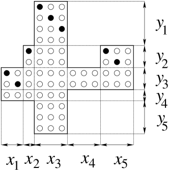
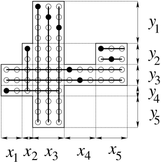
Refer back to Figure 10. Subdivide the region by the $n$ vertical chords through its $n$ vertices, resulting into at most $n$ vertical strips $X_{1},\ldots,X_{n}$, of widths $x_{1},\ldots,x_{n}$. Similarly, consider a subdivision by the $n$ horizontal chords through the $n$ vertices into at most $n$ horizontal strips $Y_{1},\ldots,Y_{n}$, of width $y_{1},\ldots,y_{n}$. In total, we get a subdivision into at most $n^{2}$ cells $C_{ij}$. Despite of this quadratic number of cells, we can deal with the overall problem in near-linear time: Note that both subdivisions can be found in time $O(n\log n)$. For the case of a connected boundary, Chazelle’s linear-time triangulation algorithm [12] implies a complexity of $O(n)$.

Choose any cell $C_{ij}$, which is a rectangle of size $x_{i}\times y_{j}$. Then $r_{ij}=\min\{x_{i},y_{j}\}$ rooks can be placed greedily along the diagonal of $C_{ij}$, without causing any interference; such a set of rooks can be encoded as one “fat” rook, described by its leftmost uppermost corner $(\xi_{ij},\eta_{ij})$, and its width $r_{ij}$. Then the strip $X_{i}$ can contain at most $x_{i}-r_{ij}$ additional rooks, and $Y_{j}$ can contain at most $y_{j}-r_{ij}$ rooks. Therefore, replace $x_{i}$ by $x_{i}-r_{ij}$, and $y_{j}$ by $y_{j}-r_{ij}$. This changes the width of at least one of the strips to zero, effectively removing it from the set of strips. After at most $2n-1$ steps of this type, all horizontal or all vertical strips have been removed, implying that we have a maximal greedy rook cover.

It is straightforward to see that for a fat rook at position $(\xi_{ij},\eta_{ij})$ and width $r_{ij}$, there is a canonical set of $r_{ij}$ cycles with $10$ edges each that covers every pixel that can be attacked from this rook. Furthermore, there is a “fat” cycle with at most $12r_{ij}-2$ turns that is obtained by a canonical merging of the $r_{ij}$ small cycles. Finally, it is straightforward to merge the fat cycles. ∎

If we are willing to invest more time for computation, we can find an optimal rook cover (instead of a greedy one). As discussed in the proof of Lemma 13, this optimal rook cover yields an optimal strip cover. An optimal strip cover can be used to get a $6$-approximation, and the new running time is $O(n^{2.5}\log n)$ or $O(N^{2.376})$.

Theorem 21.

There is an $O(n^{2.5}\log N)$-time or $O(N^{2.376})$-time algorithm that computes a milling tour with number of turns within $6$ times the optimal, and with length within $4$ times the optimal.

Proof.

Apply Lemma 13 to find an optimal strip cover of the region. (See Figure 10.) As described in the proof of that lemma, the cardinality of an optimal strip cover is equal to the cardinality of an optimal rook cover. As stated, the number of strips is a lower bound on the number of turns in a cycle cover or tour.

Now any strip from $u$ to $w$ is covered by a “doubling” cycle with edges $(u,w)$, $(w,w)$, $(w,u)$, $(u,u)$. This gives a $4$-approximation to minimum-turn cycle covers. Finally apply Corollary 10 to get a $6$-approximation to minimum-turn tours.

The claim about coverage (and hence overall length) follows from the fact that an optimal strip cover has maximum coverage 2, hence the cycle cover has maximum coverage 4. ∎

By more sophisticated merging procedures, it is possible to reduce the approximation factor for tours to a figure closer to $4$. Note that in the case of $N$ being large compared to $n$, the above proof grossly overestimates the cost of merging, as all cycles within a fat strip allow merging at no additional cost. However, our best approximation algorithm achieves a factor less than $4$ and uses a different strategy.

Theorem 22.

For an integral orthogonal polygon with $n$ edges and $N$ pixels, there are $2.5$-approximation algorithms, with running times $O(N^{2.376}+n^{3})$ and $O(n^{2.5}\log N+n^{3})$, for minimum-turn cycle cover, and hence there is a polynomial-time $3.75$-approximation for minimum-turn tours.

Proof.

As described in Lemma 13, find an optimal strip cover $S$, in time $O(N^{2.376})$ or $O(n^{2.5}\log N)$. Let $s$ be its cardinality and let opt be the cost of an optimal tour, then opt$\geq s$.

Now consider the end vertices of the strip cover. By construction, they are part of the boundary. Because any feasible tour $T$ must encounter each pixel, and cannot cross the boundary, any endpoint of a strip is either crossed orthogonally, or the tour turns at the boundary segment. In any case, a tour must have an edge that crosses an end vertex orthogonally to the strip. (Note that this edge has zero length in case of a U-turn.)

As in Section 4.1 and the proof of Theorem 19, define a weight function between endpoints of strips, taking into account the direction when leaving a strip. Again any feasible tour consists of two different matchings $M_{1}$ and $M_{2}$ between strip endpoints, and for an optimal matching $M$, we have $d(M)\leq$ opt$/2$.

Computing such a matching can be achieved as follows. Note that for $N$ pixels, an optimal strip cover has $O(\min\{\sqrt{N},n\})$ strips; by matching endpoints of neighboring strips within the same fat strip, we are left with $O(n)$ endpoints. As described in the proof of Lemma 13, the overall cost for computing the link distance between all pairs of endpoints can be achieved in $O(\min\{N\log N,n^{2}\log n\})$. Computing a minimum-weight perfect matching can be achieved in time $O(\max\{N^{1.5},n^{3}\})$.

The edges of $M$ and the strips of $S$ induce a 2-factor of the endpoints. Because any matching edges leaves a strip orthogonally, we get at most 2 additional turns at each strip for turning each 2-factor into a cycle. The total number of turns is $2s+w(M)\leq 2.5\cdot$opt. Because the strips cover the whole region, we get a feasible cycle cover.

Finally, we can use Corollary 10 to turn the cycle cover into a tour. By the corollary, this tour does not have more than $3.75\cdot$opt turns. ∎

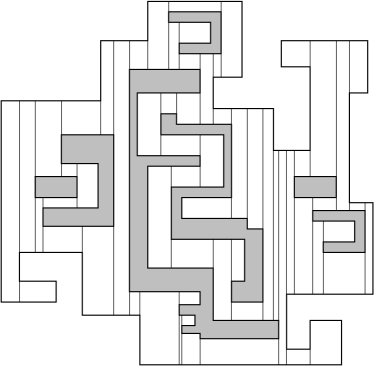
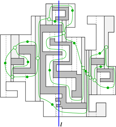
The class of examples in Example 23 shows that the cycle cover algorithm may use $2\cdot$opt turns, and the tour algorithm may use $3\cdot$opt turns, assuming that no special algorithms are used for matching and merging. Moreover, the same example shows that this $3.75$-approximation algorithm does not give an immediate length bound on the resulting tour:

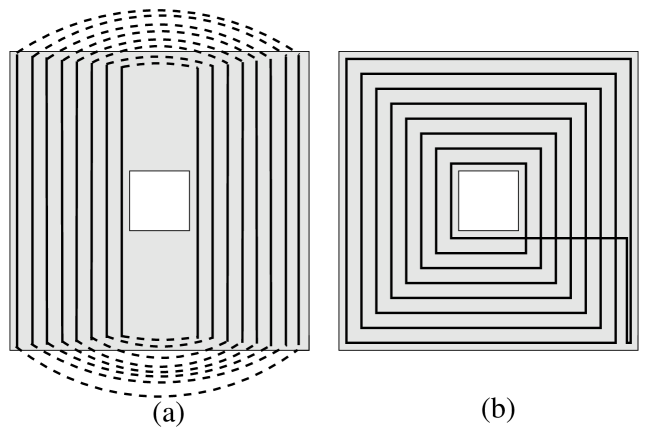
Example 23.

The class of regions shown in Figure 12 may yield a heuristic cycle cover with $2\cdot$opt turns, and a heuristic tour with $3\cdot$opt turns.

The region consists of a “square donut” of width $k$. An optimal strip cover consists of $4k$ strips; an optimal matching of strip ends yields a total of $8k+2$ turns, and we get a total of $2k$ cycles. (In Figure 12(a), only the vertical strips and their matching edges are shown to keep the drawing cleaner.) If the merging of these cycles is done badly (by merging cycles at crossings and not at parallel edges), it may cost another $4k-2$ turns, for a total of $12k$ turns. As can be seen from Figure 12(b), there is a feasible tour that uses only $4k+2$ turns. This shows that optimal tours may have almost all turns strictly inside of the region. Moreover, the same example shows that this $3.75$-approximation algorithm does not give an immediate length bound on the resulting tour. However, we can use a local modification argument to show the following:

Figure 12: A bad example for the 3.75-approximation algorithm: (a) Half the cycles constructed by the algorithm. (b) An optimal tour.

Theorem 24.

For any given feasible tour (or cycle cover) of an integral orthogonal region, there is a feasible tour (or cycle cover) of equal turn number that covers each pixel at most four times. This implies a performance ratio of 4 on the total length.

Proof.

See Figure 13. Suppose there is a pixel that is covered at least five times. Then there is a direction (say, horizontal) in which it is covered at least three times. Let there be three horizontal segments $(1,1^{\prime})$, $(2,2^{\prime})$, $(3,3^{\prime})$ covering the same pixel, as shown in Figure 13(a); we denote by $1$, $2$, $3$ the endpoints to the left of the pixel, and by $1^{\prime}$, $2^{\prime}$, $3^{\prime}$ the endpoints to the right of the pixel.

Now consider the connections of these points by the rest of the tour, i.e., a second matching between the points $1$, $2$, $3$, $1^{\prime}$, $2^{\prime}$, $3^{\prime}$ that forms a cycle, when merged with the first matching $(1,1^{\prime})$, $(2,2^{\prime})$, $(3,3^{\prime})$. This second matching is shown dashed in Figure 13(b,c). We consider two cases, depending on the structure of the second matching.

In the first case, there are two right endpoints that are matched, say $1^{\prime}$ and $2^{\prime}$. Then there must be two left endpoints that are matched; because both matchings must form one large cycle, these cannot be $1$ and $2$. Without loss of generality, we may assume they are $1$ and $3$. Thus, $2$ and $3^{\prime}$ must be matched, as shown in Figure 13(b). Then we can replace $(1,1^{\prime})$, $(2,2^{\prime})$, $(3,3^{\prime})$ by $(1,2^{\prime})$, $(2,3)$, $(1^{\prime},3^{\prime})$, respectively, which yields a feasible tour with the same number of turns, but with some pixels being covered fewer times, and no pixel being covered more times than was the case in the original tour.

In the other case, all right endpoints are matched with left endpoints. Clearly, $1^{\prime}$ cannot be matched with 1; without loss of generality, we assume it is matched with 2, as shown in Figure 13(c). Then the cycle condition implies that the second matching is $(1,3^{\prime})$, $(2,1^{\prime})$, $(3,2^{\prime})$. This allows us to replace $(1,1^{\prime})$, $(2,2^{\prime})$, $(3,3^{\prime})$ by $(1,3)$, $(2,3^{\prime})$, $(1^{\prime},2^{\prime})$, respectively, again producing a feasible tour with the same number of turns, but with some pixels being covered fewer times, and no pixel being covered more times than was the case in the original tour.

This can be repeated until no pixel is covered more than four times. As the above procedure can be carried out as part of the merging phase (i.e., after an optimal weighted matching has been found), the overall complexity is not affected. Furthermore, it is straightforward to see that it also works for the case of “thick” strips, where $N$ is large compared to $n$, by treating parallel edges in a thick strip simultaneously. ∎

Figure 13: Rearranging a tour to ensure that no pixel is covered more than three times in each direction: (a) A set of horizontal edges that covers some pixel three times. (b) A rearranged tour, if the second matching between endpoints connects two left and two right endpoints. (c) A rearranged tour, if the second matching between endpoints connects any left with a right endpoint.

5.3 Nonintegral Orthogonal Polygons

Nonintegral orthogonal polygons present a difficulty in that no polynomial-time algorithm is known to compute a minimum strip cover for such polygons. Fortunately, however, we can use the boundary tours from Section 4.1 to the approximation factor of $12$ from Theorem 20 for the integral orthogonal case.

Theorem 25.

In nonintegral orthogonal milling of a polygonal region with $n$ edges and $N$ pixels, there is a polynomial-time $4.5$-approximation for minimum-turn cycle covers and $6.25$-approximation for minimum-turn tours, with a simultaneous performance guarantee of 8 on length and cover number. The running time is $O(N^{2.376}+n^{3})$, or $O(n^{2.5}\log N+n^{3})$.

Proof.

Take the $2.5$-approximate cycle cover of the integral pixels in the region as in Theorem 22; for a tour, turn it into a $3.75$-approximate tour. This may leave a fractional portion along the boundary uncovered. See Figure 14.

Figure 14: Milling a nonintegral orthogonal polygon

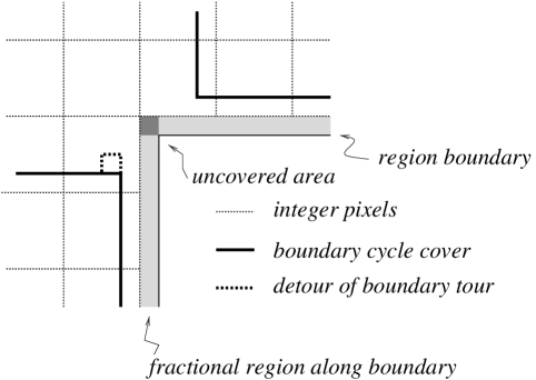
Now add in an optimal cycle cover of the boundary which comes from Theorem 6. This may only leave fractional boundary pieces uncovered that are near reflex vertices of the boundary, as shown in Figure 14. Whenever this happens, there must be a turn of the boundary cycle cover on both side of the reflex vertex. The fractional patch can be covered at the cost of an extra two turns, which are charged to the two turns in the boundary cycles. Therefore, the modified boundary cover has a cost of at most $2\cdot$opt. Compared to an optimal cycle cover of length opt, we get a cycle cover of length at most $4.5\cdot$opt, as claimed. For an optimal tour of length opt, merging all modified boundary cycles into one cycle can be done at a cost of at most 2 turns per unmodified boundary cycle, i.e., for a total of $\frac{1}{2}\cdot$opt.

Finally, the remaining two cycles can be merged at a cost of 2 turns. This yields an overall approximation factor of $3.75+2.5=6.25$. The claim on the cover number (and thus length) follows from applying Theorem 24 to each of the two cycles.

The running times follow from Theorems 6 and 22. ∎

5.4 Milling Thin Orthogonal Polygons

In this section we consider the special case of milling thin polygons. Again, we focus on the integral orthogonal case. Formally, a thin polygon is one in which no axis-aligned 2$\times$2 square fits, implying that each pixel has all four of its corners on the boundary of the polygon. Intuitively, a polygon is thin if it is composed of a network of width-1 corridors, where each pixel is adjacent to some part of the boundary of the region, making this related to discrete milling.

5.4.1 Basics of Thin Orthogonal Polygons

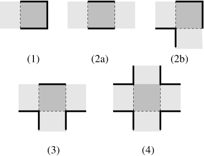
Any pixel in the polygon has one, two, three or four neighbor pixels; we denote this number of neighbors as the degree of a pixel. See Figure 15. Degree one pixels (1) are “dead ends”, where the cutter has to make a u-turn. There are two types of degree two pixels, without forcing a turn (2a) or with forcing a turn (2b); in either case, applying Lemma 5 in an appropriate manner will suggest that they should be visited in a canonical way: after one neighbor, and before the other. Neighbors of degree three pixels (3) form “T” intersections that force duplication of paths. Degree four pixels (4) are the only pixels in thin polygons that are not boundary pixels as defined in Section 4; however, in the absence of 2$\times$2 squares of pixels, all their neighbors are of degree one or two.

Figure 15: Pixel types in a thin polygon.

In the following, we will use the ideas developed for boundary cycle covers in Section 4.1 to obtain cycle covers for thin polygons. The following is a straightforward consequence of Theorem 6 and Theorem 9.

Corollary 26.

In thin orthogonal milling, there is an $O(n^{3})$ algorithm for computing a minimum-turn cycle cover, and an $O(n^{3})$ 1.5-approximation for computing a minimum-turn tour.

Proof.

Apply the strongly polynomial algorithm described in Theorem 6 for computing a minimum cost boundary cycle cover. By definition, this covers all pixels of degree one, two, and three. Moreover, degree four pixels are surrounded by pixels of degree one or two, implying that they are automatically covered as neighbors of those pixels, when applying Lemma 5. Using Theorem 9, we can turn this into a tour, yielding the claimed approximation factor. ∎

More interesting is that we can do much better than general merging in the case of thin orthogonal milling. The idea is to decompose the induced graph into a number of cheap cycles, and a number of paths.

5.4.2 Milling Thin Eulerian Orthogonal Polygons

We first solve the special case of milling Eulerian polygons, that is, polygons that can be milled without retracing edges of the tour, so that each edge in the induced graph is traversed by the cutting tool exactly once. In an Eulerian polygon, all pixels have either two or four neighbors, meaning there are no odd-degree pixels.

Although one might expect that the optimal milling is one of the possible Eulerian tours of the graph, in fact, this is not always true, as Example 27 points out.

Example 27.

There exist thin grid graphs, such that no turn-minimal tour of the graph is an Eulerian tour.

Figure 16: A thin Eulerian polygon consisting of four overlapping cycles (above). Shown symbolically below is how to obtain an overall tour by merging the four canonical cycles: A tour obtained by iteratively merging cycles incurs a total of 16+6=22 turns (bottom left). An optimal tour has 16+4=20 turns (bottom right).

Proof.

See Figure 16. Observe that an optimal milling is not an Eulerian Tour. The best Eulerian Tour for this figure requires 22 turns, as shown symbolically in the bottom left of the figure: Each cycle uses 4 turns and an additional 6 turns can be used to connect the four cycles together. On the other hand, the optimal milling traverses the edges in the internal pixel twice, both times in the same direction: The order of turns is $1,2,C,13,16,15,14,D,9,12,11,10,B,5,8,7,6,A,3,4,1$, and the structure is shown symbolically in the bottom right. Thus, the optimal milling only requires 20 turns, where each cycle uses 4 turns and an additional 4 turns connect the cycles together. ∎

By strengthening the lower bound, we can achieve the following approximation of an optimal tour of length opt:

Theorem 28.

There is an $O(n\log n)$ (or $O(N)$) algorithm that finds a tour of turn cost at most $\frac{6}{5}\cdot$opt.

Proof.

By applying Theorem 6, we get an optimal boundary cycle cover. There are three observations that lead to the claimed stronger results.

(1) For a thin polygon, extracting the collinear strips can be performed in strongly polynomial time $O(n\log)$ (or weakly polynomial time $O(N)$).

(2) For an Eulerian thin polygon, no vertices in $G_{\overline{P}}$ remain unmatched after repeatedly applying Lemma 5. Instead, we get an optimal cycle cover right away. This cycle cover can be merged into one connecting tour by merging at pixels where two cycles cross each other: Let the optimal cycle cover be composed of $c$ disjoint cycles, where $c\geq 1$. Let $t$ be the cost of the optimal cycle cover. At each phase of the cycle-merging algorithm, two cycles are merged into one. Therefore, the algorithm finds a solution having cost $t+2\cdot(c-1)$.

(3) We can strengthen the lower bound on an optimal tour as follows. Consider (for $c>1$) a lower bound on the cost of the optimal solution. Just like in the proof of Theorem 1, all turns in a cycle cover are forced by convex corners of the polygon, implying that any solution must contain these $t$ turns. In addition, turning from one cycle into another incurs a crossing cost of at least one turn; thus, we get a lower bound of $t+c$. Observe that there are at least $4$ turns per cycle so that $t\geq 4c$. Therefore, $\frac{t+2\cdot(c-1)}{t+c}\leq\frac{t+2c}{t+c}\leq\frac{6}{5}$. ∎

5.4.3 Milling Arbitrary Thin Orthogonal Polygons

Now we consider the case of general thin polygons. For any odd-degree vertex, and any feasible solution, some edges may have to be traversed multiple times. As in Corollary 26, we can apply Theorem 6 to achieve a minimum-cost cycle cover and merge them into a tour. Using a more refined analysis, we can use this to obtain a $4/3$-approximation algorithm for finding an minimum-cost tour.

Theorem 29.

For thin orthogonal milling, we can compute a tour of turn cost at most $\frac{4}{3}\cdot$opt in time $O(n^{3})$, where opt is the cost of an optimal tour.

Proof.

We start by describing how to merge the cycles into one connected tour.

1. find an optimal cycle cover as provided by Theorem 6;

2. repeat until there is only one cycle in the cycle cover:

   • If there are any two cycles that can be merged without any extra cost (by having partially overlapping collinear edges), perform the merge.

   • Otherwise,

     • Find a vertex at which two cycles cross each other.

     • Modify the vertex to incorporate at most two additional turns, thereby connecting the two cycles.

Now we analyze the performance of our algorithm. Consider the situation after extracting the cost zero matching edges from Lemma 5. This already yields a set $K$ of cycles, obtained by only turning at pixels of degree two that force a turn. Let $k$ denote the number of cycles in $K$, and $c$ be the number of turns in $K$. Let $P$ be the set of “dangling” paths at degree-one or degree-three pixels, and let $p$ be the number of turns in $P$, including the mandatory turn for each endpoint. Let $M$ be a minimum matching between odd-degree vertices, and let $m$ be the number of turns in $M$. Finally, let $O$ be the matching between odd-degree pixels that is induced by an optimal tour, and let $o$ be the number of turns in $O$.

First note that $P$ is a matching between odd-degree nodes.

$P$, $M$ and $O$ may connect some of the cycles in $K$. In $P$ a path between two odd-degree pixels connects the two cycles that the two nodes belong to. On the other hand, a path in $M$ and $O$ between two odd-degree nodes can encounter several cycles along the way, and thus it may be used to merge several cycles at no extra cost.

Therefore, let $j$ be the number of cycles after using $P$ for free merging, let $i$ be the number of components with $P$ and $M$ used for free merging, and let $h$ be the number of components with $P$ and $O$ used for free merging.

Note that

$$1\leq i\leq j\leq k,$$ (1)

and

$$1\leq h\leq j\leq k.$$ (2)

Now consider the number of cycles encountered by a path in the matching. It is not hard to see that this number cannot exceed the number of its turns. Therefore,

$$m\geq k-i\geq j-i$$ (3)

$$o\geq k-h\geq j-h$$ (4)

If a particular matching results in $x$ components, we would need at least another $x$ turns to get a tour. Thus with $O$ we need at least $h$ more turns.

Thus, for an optimal tour of cost opt, we have

$$\mbox{\sc opt}\geq c+p+o+h.$$ (5)

Our heuristic method adds the minimum matching to $C$ and $P$ and merges the remaining components with two turns per merge, hence the cost heur of the resulting tour is

$$\mbox{\sc heur}\geq c+p+m+2(i-1).$$ (6)

Thus we get the following estimate for the approximation factor $R\geq 1$:

$$R\leq\frac{c+p+m+2i}{c+p+o+h}$$ (7)

Because each cycle has at least four turns, we know that

$$c\geq 4k\geq 4j.$$ (8)

Using the fact that $c+p+m+2i\geq c+p+o+h$ (because $R\geq 1$), we see that the ratio on the right in (7) gets larger if we replace $c$ in the numerator and in the denominator by the smaller nonnegative value $4j$; thus,

$$R\leq\frac{4j+p+m+2i}{4j+p+o+h}.$$ (9)

Because $P$ is also a matching, we have

$$p\geq m,$$ (10)

which implies that

$$R\leq\frac{4j+2m+2i}{4j+m+o+h}.$$ (11)

We also know that

$$m\leq o.$$ (12)

Using this, together with the fact that $R$ can be assumed to be less than 2, we can argue that $R$ is maximal for maximal values of $m$; hence,

$$R\leq\frac{4j+2o+2i}{4j+2o+h}.$$ (13)

Using (4) in (13), we see that $R$ is maximal for minimal $o$; hence,

$$R\leq\frac{4j+2(j-h)+2i}{4j+2(j-h)+h}=\frac{6j-2h+2i}{6j-h}.$$ (14)

Using $h>o$ in (14) and the facts that $R<2$ and $i\leq j$, we get that

$$R\leq\frac{6j-2o+2i}{6j-o}\leq\frac{6j+2i}{6j}\leq\frac{4}{3}.$$ (15)

∎

The following shows that the estimate for the performance ratio is tight.

Theorem 30.

There is a class of examples for which the estimate of 4/3 for the performance ratio of the algorithm for thin orthogonal milling is tight.

Proof.

See Figure 17. The region consists of $k=2s+4$ cycles, all with precisely 4 turns, $s$ cycles without degree-three vertices, and $s+4$ cycles with two degree-three vertices each. We get $c=4k=8s+16$ and $p=2(s+4)=2s+8$. Figure 17(b) shows a min-cost matching of cost $m=2(s+4)=2s+8$ and one of cost $o=2s+8$ that is induced by an optimum tour. As Figure 17(c) suggests, merging all cycles, odd-degree paths and matching paths is possible without requiring any further turns, resulting in $\mbox{\sc opt}=c+p+o=12s+32$. On the other hand, using the min-cost matching of cost $m$ leaves $k$ cycles that cannot be merged for free; thus, merging two cycles at a time at a cost of 2 turns requires an additional cost of $2(k-1)=4s+6$, for a total of $\mbox{\sc heur}=c+p+m+2(k-1)=16s+38$ turns, which gets arbitrarily close to $\frac{4}{3}\mbox{\sc opt}$ for large $s$. ∎

Figure 17: An example with performance ratio 4/3 for our heuristic. (a) The structure of the example for $s=8$. (b) A min-cost matching of the odd-degree vertices, and the matching induced by an optimal tour. (c) A portion of the optimal tour: Subtours can be merged without extra cost. (d) A corresponding portion of the heuristic tour: Subtours still need to be merged, which results in an additional cost of $2(k-1)=4s+6$.

Note that the argument of Theorem 24 remains valid for this section, so the bounds on coverage and length approximation still apply.

5.5 PTAS

We describe a polynomial-time approximation scheme (PTAS) for the problem of minimizing a weighted average of the two cost criteria: length and number of turns. Our technique is based on using the theory of $m$-guillotine subdivisions [38], properly extended to handle turn costs. We prove the following result:

Theorem 31.

Define the cost of a tour to be its length plus $C$ times the number of (90-degree) turns. For any fixed $\varepsilon>0$, there is a $(1+\varepsilon)$-approximation algorithm, with running time $2^{O(h)}\cdot N^{O(C)}$, for minimizing the cost of a tour for an integral orthogonal polygon $P$ with $h$ holes and $N$ pixels.

Proof.

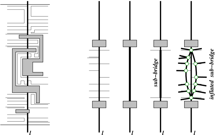
Let $T^{*}$ be a minimum-cost tour and let $m$ be any positive integer. Following the notation of [38], we first apply the main structure theorem of that paper to claim that there is an $m$-guillotine subdivision, $T_{G}$, obtained from $T^{*}$ by adding an appropriate set of bridges ($m$-spans, which are horizontal or vertical segments) of total length at most ${1\over m}|T^{*}|$, with length at most $(1+{1\over m})$ times the length of $T^{*}$. (Because $T^{*}$ may traverse a horizontal/vertical segment twice, we consider such segments to have multiplicities (1 or 2), as multi-edges in a graph.)

We note that part of $T_{G}$ may lie outside the polygon $P$, because the $m$-spans that we add to make $T^{*}$ $m$-guillotine need not lie within $P$. We convert $T_{G}$ into a new graph by subtracting those portions of each bridge that lie outside of $P$. In this way, each bridge of $T_{G}$ becomes a set of segments within $P$; we trim each such segment at the first and last edge of $T_{G}$ that is incident on it and call the resulting trimmed segments sub-bridges. (Note that a sub-bridge may be a single point if the corresponding segment is incident on a single edge of $T^{*}$; we can ignore such trivial sub-bridges.) As in the TSP method of [38], we double the (non-trivial) sub-bridges: We replace each sub-bridge by a pair of coincident segments, which we “inflate” slightly to form a degenerate loop, such that the endpoints of the sub-bridge become vertices of degree four, and the endpoints of each edge incident on the interior of the sub-bridge become vertices of degree three (which occur in pairs). Refer to Figure 18. We let $T_{G}^{\prime}$ denote the resulting graph. Now $T_{G}^{\prime}\subset P$, and, because $T_{G}^{\prime}$ is obtained from $T^{*}$, a tour, we know that the number of odd-degree vertices of $T_{G}^{\prime}$ that lie on any one sub-bridge is even (the degree-three vertices along a sub-bridge come in pairs).

Figure 18: Definitions of sub-bridges and the graph $T_{G}^{\prime}$. A vertical line $l$ is shown, which defines a cut. The slice of an optimal solution along $l$ is shown, with thinner lines drawn along the edges of the solution (which is not intended to be an accurate instance of an optimal solution, but is drawn to illustrate some of the possible cases). Also shown is an enlargement of one portion of the cut $l$, showing a segment of the $m$-span between two portions of the boundary of $P$, the trimmed segment that forms the sub-bridge, and the portion of the resulting graph $T_{G}^{\prime}$ in the vicinity of the inflated sub-bridge.

The cost of the optimal solution $T^{*}$ is its length, $|T^{*}|$, plus $C$ times the number of its vertices. We consider the cost of $T_{G}^{\prime}$ to be also its (Euclidean) length plus $C$ times the number of its vertices. Because the number of vertices on the sub-bridges is proportional to their total length, and each edge multiplicity is at most two, we see that the cost of $T_{G}^{\prime}$ is $O((1+C)/m)\cdot|T^{*}|$ greater than the optimal cost, i.e., the cost of $T^{*}$.

In order to avoid exponential dependence on $n$ in our algorithm, we need to introduce a subdivision of $P$ that allows us to consider the sub-bridges along an $m$-span to be grouped into a relatively small ($O(h)$) number of classes. We now describe this subdivision of $P$.

By standard plane sweep with a vertical line, we partition $P$ into rectangles, using vertical chords, according to the vertical decomposition; see Figure 19(a). We then decompose $P$ into a set of $O(h)$ regions, each of which is either a “junction” or a “corridor.” This decomposition is analogous to the corridor structure of polygons that has been utilized in computing shortest paths and minimum-link separators (see, e.g., [32, 33, 40]), with the primary difference being that we use the vertical decomposition into rectangles, rather than a triangulation, as the basis of the definition. Consider the (planar) dual graph, ${\cal G}$, of the vertical partition of $P$; the nodes of ${\cal G}$ are the rectangles, and two nodes are joined by an edge if and only if they are adjacent. We now define a process to transform the vertical decomposition into our desired decomposition. First, we take any degree-1 node of ${\cal G}$ and delete it, along with its incident edge; in the vertical decomposition, we remove the corresponding vertical chord (dual to the edge of ${\cal G}$ that was deleted). We repeat this process, merging a degree-1 region with its neighbor, until there are no degree-1 nodes in ${\cal G}$. At this stage, ${\cal G}$ has $h+1$ faces and all nodes are of degree 2 or more. Assume that $h\geq 2$ (the case $h\leq 1$ is easy); then, not all nodes are of degree 2, implying that there are at least two higher-degree nodes. Next, for each pair of adjacent degree-2 nodes, we merge the nodes, deleting the edge between them, and removing the corresponding vertical chord separating them in the decomposition. The final dual graph ${\cal G}$ has nodes of two types: those that are dual to regions of degree 2, which we call the corridors, and those that are dual to regions of degree greater than 2, which we call the junctions. Each corridor is bounded by exactly two vertical chords, together with two portions of the boundary of $P$. (These two portions may, in fact, come from the same connected component of the boundary of $P$.) Each of the $h$ bounded faces of ${\cal G}$ contains exactly one of the holes of $P$. Refer to Figure 19.

(a) (b)

Figure 19: (a). The vertical decomposition of $P$ (holes in dark grey). (b). The decomposition of $P$ into junctions (light grey) and corridors, with the dual graph overlaid. The nodes of the dual graph are shown hollow for junctions and shown as smaller solid disks for the corridors.

Let ${\cal V}$ denote the decomposition of $P$ just described; there is an analogous horizontal partition, ${\cal H}$, of $P$ into $O(h)$ regions. The vertical sub-bridges of a vertical bridge are partitioned into $O(h)$ classes according to the identity of the region, $\tau$, that contains the sub-bridge in the vertical decomposition ${\cal V}$. A sub-bridge intersecting a region $\tau$ of ${\cal V}$ is called separating if it separates some pair of vertical chords on the boundary of $\tau$; it is trivial otherwise. (Corridor regions have only two vertical chords on their boundary, while junctions may have several, as many as $\Theta(h)$ in degenerate cases.)

First, consider a corridor region $\tau$ in ${\cal V}$, and let $a$ and $b$ denote the two vertical chords that bound it. An important observation regarding sub-bridge classes in corridors is this: The parity of the number of times a tour crosses $a$ must be the same as the parity of the number of times a tour crosses $b$. The consequence is that we can specify the parity of the number of incidences on all separating sub-bridges of a given corridor class by specifying the parity of the number of incidences on a single sub-bridge of the class; the trivial sub-bridges always have an even parity of crossing.

Now consider a junction region $\tau$ in ${\cal V}$. Because, in the merging process that defines ${\cal V}$, we never merge a degree-2 region with a higher-degree region, we know that $\tau$ consists of a single high-degree ($>2$) rectangle, $R_{\tau}$, from the original vertical decomposition, together with possibly many other rectangles that form a “pocket” attached to $R_{\tau}$, corresponding to a tree in the dual graph (so that removal of degree-1 nodes leads to a collapse of the tree and a merging of the pocket to $R_{\tau}$). The consequence of this observation is that there can be at most one separating sub-bridge in a junction class. (There may be several trivial sub-bridges.)

Our algorithm applies dynamic programming to obtain a minimum-cost $m$-guillotine subdivision, $T_{G}^{*}$, from among all those $m$-guillotine subdivisions that have the following additional properties:

(1)

It consists of a union of horizontal/vertical segments, having half-integral coordinates, within $P$.

(2)

It is connected.

(3)

It covers $P$, in that the center of every pixel of $P$ is intersected by an edge of the subdivision.

(4)

It is a bridge-doubled $m$-guillotine subdivision, so that every (non-trivial) sub-bridge of an $m$-span appears twice (as a multi-edge).

(5)

It interconnects the sub-bridges in each of a specified partition of the classes of sub-bridges.

(6)

It obeys a parity constraint on each of the $O(h)$ classes of sub-bridges: The number of edges of the subdivision incident on each separating sub-bridge of the class corresponding to a region $\tau$ is even or odd, according to the specified parity for $\tau$.

A subproblem in the dynamic programming algorithm is specified by a rectangle, having half-integral coordinates, together with boundary information associated with the rectangle, which specifies how the subdivision within the rectangle interacts with the subdivision outside the rectangle. The boundary information includes (a) $O(m)$ attachment points, where edges meet the boundary at points other than along the $m$-span; (b) the multiplicity (1 or 2) of each attachment point, and the interconnection pattern (if any) of adjacent attachment points along the rectangle boundary; (c) the endpoints of a bridge on each side of the rectangle (from which one can deduce the sub-bridges); (d) interconnection requirements among the attachment points and the classes of sub-bridges; and (e) a parity bit for each class of sub-bridge, indicating whether an even or an odd number of edges should be incident to the separating sub-bridges of that class. There are $N^{O(m)}\cdot 2^{O(h)}$ subproblems. At the base of the dynamic programming recursion are rectangles of constant size (e.g., unit squares).

The optimization considers each possible cut (horizontal or vertical, at half-integral coordinates) for a given subproblem, together with all possible choices for the new boundary information along the cut, and minimizes the total resulting cost, adding the costs of the two resulting subproblems to the cost of the choices made at the cut (which includes the length of edges added, plus $C$ times the number of vertices added).

Once an optimal subdivision, $T_{G}^{*}$, is computed, we can recover a valid tour from it by extracting an Eulerian subgraph obtained by removing a subset of the edges on each doubled sub-bridge. The parity conditions imply that such an Eulerian subgraph exists. An Eulerian tour on this subgraph is a covering tour, and its cost is at most $O(C/m)\cdot|T^{*}|$ greater than optimal. For any fixed $\varepsilon>0$, we set $m=\lceil C/\varepsilon\rceil$, resulting in a $(1+\varepsilon)$-approximation algorithm with running time $O(N^{O(C/\varepsilon)}\cdot 2^{O(h)}$. The techniques of [38], which use “grid-rounded” $m$-guillotine subdivisions, can be applied to reduce the exponent on $N$ to a term, $O(C)$, independent of $m$. ∎

Remarks

It should be possible to apply a variant of our methods to obtain a PTAS that is polynomial in $n$ (versus $N$), with a careful consideration of implicit encodings of tours. We note that our result relies on effectively “charging off” turn cost to path length, because the objective function is a linear combination of the two costs (turns and length). We have not yet been able to give a PTAS for minimizing only the number of turns in a covering tour; this remains an intriguing open problem.

6 Conclusion

We have presented a variety of results for finding an optimal tour with turn cost. Many open problems remain. The most curious seems to be the following, which highlights the difference between turn cost and length, as well as the difference between a cycle cover and a 2-factor:

Problem 32.

What is the complexity of finding a minimum-turn cycle cover in a grid graph?

This problem has been open for several years now; in fact, it is Problem # 53 on the well-known list [17], known as “The Open Problems Project”. Finding a minimum weighted turn cycle cover is known to be NP-hard for a set of points in the plane [1]; however, the proof uses the fact that there are more than two directions for the edges in a convex cycle. While we tend to believe that Problem 32 may have the answer “NP-complete”, a polynomial solution would immediately lead to a 1.5-approximation for the orthogonal case, and a $(1+{2\over 3})$-approximation for the general case.

For various optimization problems dealing with geometric regions, there is a notable difference in complexity between a region with holes, and a simple region that does not have any holes. (In particular, it can be decided in polynomial time whether a given grid graph without holes has a Hamiltonian cycle [44], even though the complexity of the TSP on these graphs is still open.) Our NP-hardness proof makes strong use of holes; furthermore, the complexity of the PTAS described above is exponential in the number of holes. This raises the following natural question.

Problem 33.

Is there a polynomial-time algorithm for exactly computing a minimum-turn covering tour for simple orthogonal polygons?

It may be possible to improve the performance of some of our approximation algorithms. In particular, the following remains unclear.

Problem 34.

Is the analysis of the 3.75-approximation algorithm tight?

We believe that it may be possible to improve the factor. We also believe that there is room for improvement in approximating nonintegral orthogonal milling, in particular by improving the cost of finding a strip cover.

Problem 35.

What is the complexity of computing a minimum strip cover in nonintegral orthogonal polygons?

An important tool for our approximation algorithms is a strip cover of small cost; finding a strip cover remains a possible approach even if strips may be parallel to more than two directions. This is closely related to other decomposition problems; see [34] for a survey.

Problem 36.

What is the complexity of computing minimum strip covers in nonorthogonal polygons?

The answer may very well be “NP-hard, even for three directions”: Hassin and Megiddo [26] show that the problem of hitting a set of points with a minimum number of lines with three slopes is hard. However, their proof constructs a disconnected set of grid points and cannot be applied directly to milling problems. In any case, even an approximation would be of interest; in particular, if it achieves the following property:

Problem 37.

Is there a strip cover approximation algorithm for $d$ directions whose performance ratio is independent of $d$?

This would imply a positive result for a special case of the following, even more general problem.

Problem 38.

Can one obtain approximation algorithms for unrestricted directions in an arbitrary polygonal domain, and an appropriately shaped cutter?

References

- [1] A. Aggarwal, D. Coppersmith, S. Khanna, R. Motwani, and B. Schieber, The angular-metric traveling salesman problem, in Proceedings of the Eighth Annual ACM-SIAM Symposium on Discrete Algorithms, Jan. 1997, pp. 221–229.
- [2] M. H. Alsuwaiyel and D. T. Lee, Minimal link visibility paths inside a simple polygon, Comput. Geom. Theory Appl., 3 (1993), pp. 1–25.
- [3] , Finding an approximate minimum-link visibility path inside a simple polygon, Inform. Process. Lett., 55 (1995), pp. 75–79.
- [4] E. M. Arkin, M. A. Bender, E. Demaine, S. P. Fekete, J. S. B. Mitchell, and S. Sethia, Optimal covering tours with turn costs, in Proc. 13th ACM-SIAM Sympos. Discrete Algorithms, 2001, pp. 138–147.
- [5] E. M. Arkin, S. P. Fekete, and J. S. B. Mitchell, The lawnmower problem, in Proc. 5th Canad. Conf. Comput. Geom., 1993, pp. 461–466.
- [6] , Approximation algorithms for lawn mowing and milling, Comput. Geom. Theory Appl., 17 (2000), pp. 25–50.
- [7] E. M. Arkin, M. Held, and C. L. Smith, Optimization problems related to zigzag pocket machining, Algorithmica, 26 (2000), pp. 197–236.
- [8] E. M. Arkin, J. S. B. Mitchell, and C. D. Piatko, Minimum-link watchman tours, Inform. Process. Lett., 86 (2003), pp. 203–207.
- [9] S. Arya, S.-W. Cheng, and D. M. Mount, Approximation algorithm for multiple-tool milling, Internat. J. Comput. Geom. Appl., 11 (2001), pp. 339–372.
- [10] A. A. Assad and B. L. Golden, Arc routing methods and applications, in Network Routing, M. O. Ball, T. L. Magnanti, C. L. Monma, and G. L. Nemhauser, eds., vol. 8 of Handbooks in Operations Research and Management Science, Elsevier Science, Amsterdam, 1995, pp. 375–483.
- [11] E. Benavent and D. Soler, The directed rural postman problem with turn penalties, Transporation Science, 33 (1999), pp. 408–418.
- [12] B. Chazelle, Triangulating a simple polygon in linear time, Discrete Comput. Geom., 6 (1991), pp. 485–524.
- [13] J. Clossey, G. Laporte, and P. Soriano, Solving arc routing problems with turn penalties, Technical Report G-2000-05, Le Groupe d’études et de recherche en analyse des décisions (GERAD), Montréal, Canada, March 2000.
- [14] M. J. Collins and B. M. E. Moret, Improved lower bounds for the link length of rectilinear spanning paths in grids, Inform. Process. Lett., 68 (1998), pp. 317–319.
- [15] J. Culberson and R. A. Reckhow, Orthogonally convex coverings of orthogonal polygons without holes, J. Comput. Syst. Sci., 39 (1989), pp. 166–204.
- [16] E. D. Demaine, M. L. Demaine, and J. S. B. Mitchell, Folding flat silhouettes and wrapping polyhedral packages: New results in computational origami, in Proc. 15th Annu. ACM Sympos. Comput. Geom., June 1999, pp. 105–114.
- [17] E. D. Demaine, J. S. B. Mitchell, and J. O’Rourke, The Open Problems Project. URL: http://maven.smith. edu/~orourke/TOPP/.
- [18] H. A. Eiselt, M. Gendreau, and G. Laporte, Arc routing problems, part I: The Chinese postman problem, Operations Research, 43 (1995), pp. 231–242.
- [19] , Arc routing problems, part II: The rural postman problem, Operations Research, 43 (1995), pp. 399–414.
- [20] S. P. Fekete, Geometry and the Travelling Salesman Problem, ph.D. thesis, Department of Combinatorics and Optimization, University of Waterloo, Waterloo, ON, 1992.
- [21] S. P. Fekete and G. J. Woeginger, Angle-restricted tours in the plane, Comput. Geom. Theory Appl., 8 (1997), pp. 195–218.
- [22] D. S. Fernández, Problemas de Rutas por Arcos con Giros Prohibidos, PhD thesis, Vniversitat de Valencia, 1995.
- [23] H. Gabow and R. Tarjan, Faster scaling algorithms for network problems, SIAM J. Comput., 18 (1989), pp. 1013–1036.
- [24] H. N. Gabow, Implementation of algorithms for maximum matching on nonbipartite graphs, PhD thesis, Department of Computer Science, Standford University, 1973.
- [25] M. R. Garey and D. S. Johnson, Computers and Intractability: A Guide to the Theory of NP-Completeness, W. H. Freeman, New York, NY, 1979.
- [26] R. Hassin and N. Megiddo, Approximation algorithms for hitting objects by straight lines, Discrete Appl. Math., 30 (1991), pp. 29–42.
- [27] M. Held, On the Computational Geometry of Pocket Machining, vol. 500 of Lecture Notes Comput. Sci., Springer-Verlag, June 1991.
- [28] O. H. Ibarra and S. Moran, Deterministic and probabilistic algorithms for maximum bipartite matching via fast matrix multiplication, Inform. Process. Lett., 13 (1981), pp. 12–15.
- [29] A. Itai, C. H. Papadimitriou, and J. L. Szwarcfiter, Hamilton paths in grid graphs, SIAM J. Comput., 11 (1982), pp. 676–686.
- [30] K. Iwano, P. Raghavan, and H. Tamaki, The traveling cameraman problem, with applications to automatic optical inspection, in Proc. 5th Annu. Internat. Sympos. Algorithms Comput., vol. 834 of Lecture Notes Comput. Sci., Springer-Verlag, 1994, pp. 29–37.
- [31] D. S. Johnson and C. H. Papadimitriou, Computational complexity and the traveling salesman problem, in The Traveling Salesman Problem, E. Lawler, J. Lenstra, A. R. Kan, and D. Shmoys, eds., John Wiley & Sons, New York, 1985, pp. 68–74.
- [32] S. Kapoor and S. N. Maheshwari, Efficient algorithms for Euclidean shortest path and visibility problems with polygonal obstacles, in Proc. 4th Annu. ACM Sympos. Comput. Geom., 1988, pp. 172–182.
- [33] S. Kapoor, S. N. Maheshwari, and J. S. B. Mitchell, An efficient algorithm for Euclidean shortest paths among polygonal obstacles in the plane, Discrete Comput. Geom., 18 (1997), pp. 377–383.
- [34] J. M. Keil, Polygon decomposition, in Handbook of Computational Geometry, J.-R. Sack and J. Urrutia, eds., Elsevier Science Publishers B.V. North-Holland, Amsterdam, 2000, pp. 491–518.
- [35] R. Klein, 2000. Personal Communication.
- [36] E. Kranakis, D. Krizanc, and L. Meertens, Link length of rectilinear Hamiltonian tours on grids, Ars Combinatorica, 38 (1994), p. 177.
- [37] J. S. B. Mitchell, shortest paths among polygonal obstacles in the plane, Algorithmica, 8 (1992), pp. 55–88.
- [38] , Guillotine subdivisions approximate polygonal subdivisions: A simple polynomial-time approximation scheme for geometric TSP, -MST, and related problems, SIAM J. Comput., 28 (1999), pp. 1298–1309.
- [39] , Geometric shortest paths and network optimization, in Handbook of Computational Geometry, J.-R. Sack and J. Urrutia, eds., Elsevier Science Publishers B.V. North-Holland, Amsterdam, 2000, pp. 633–701.
- [40] J. S. B. Mitchell and S. Suri, Separation and approximation of polyhedral objects, Comput. Geom. Theory Appl., 5 (1995), pp. 95–114.
- [41] E. M. Molada and D. S. Fernández, Exact solution of the Chinese postman problem with turn penalties, in XV Congress on Differential Equations and Applications/V Congress on Applied Mathematics, vol. I, II (Spanish), Colecc. Congr., 9, 1998, pp. 1111–1115.
- [42] S. Ntafos, Watchman routes under limited visibility, Comput. Geom. Theory Appl., 1 (1992), pp. 149–170.
- [43] A. Schrijver, Combinatorial Optimization, Springer-Verlag, Berlin, 2003.
- [44] C. Umans and W. Lenhart, Hamiltonian cycles in solid grid graphs, in Proc. 38th Annu. IEEE Sympos. Found. Comput. Sci., 1997, pp. 496–507.
- [45] D. West, An Introduction to Graph Theory, Prentice Hall, 1995.