A Digital version of Green’s Theorem and its application to the coverage problem in Formal Verification

Abstract.

We present a novel scheme to the coverage problem, introducing a quantitative way to estimate the interaction between a block an its environment. This is achieved by setting a discrete version of Green’s Theorem, specially adapted for Model Checking based verification of integrated circuits.
This method is best suited for the coverage problem since it enables one to quantify the incompleteness or, on the other hand, the redundancy of a set of rules, describing the model under verification. Moreover this can be done continuously throughout the verification process, thus enabling the user to pinpoint the stages at which incompleteness/redundancy occurs.
Although the method is presented locally on a small hardware example, we additionally show its possibility to provide precise coverage estimation also for large scale systems. We compare this method to others by checking it on the same test-cases.

1. Introduction

While automatic verification methods (s.a. Model Checking, etc.) permit quite accurate formulation of rules describing concurrent systems, the coverage problem is still open. This problem can be stated as ones ability to know that a certain set of rules covers all possible behaviors of the system and if so, whether this set is optimal, in the sense that it does not contain redundancies.
This problem, besides being a very challenging research problem, also plays a crucial role in industrial implementation of verification methods, in aspects of manpower, time and, (of course, finance.
While different methods to attack this problem where proposed (see [KGG], [HKHZ], [AS]), it is still largely open.
In this paper we present a novel scheme to the coverage problem, introducing a quantitative way to estimate the interaction between a block an its environment. This is achieved by setting a discrete version of Green’s Theorem, specially adapted for Model Checking based verification.
This work was inspired by the well known principle of Model Checking that a well written environment dictates the formulation of the system’s rules; indeed the rules governing the system and the description of its physical proprieties should be regarded as almost mirror images of each other. On a more theoretical level, resides the idea of viewing a flow of information in an analogous way to the electromagnetic (or energy) flow and the computation of its mean flux, i.e. pressure. The main idea behind the results presented herein is the adaptation of the symmetry principle to the flow setting, adaptation which states that the mean pressure of information is constant, (i.e. the informational system is in dynamic equilibrium).
This method is best suited for the coverage problem since it enables one to quantify the incompleteness or, on the other hand, the redundancy of a set of rules, describing the model under verification. Moreover this can be done continuously throughout the verification process, thus enabling the user to pinpoint the stages at which incompleteness/redundancy occurs. The method we present here does not permit the complete automation of the coverage-checking process (thus making the verifier’s role redundant), since it doesn’t guarantee completeness of coverage, but only that inconsistencies or redundancies are discovered. Thus it is yet another instrument in the arsenal of the experienced verifier, and one that is extremely easily to use without any further specialization. Moreover, it can be readily added as supplementary feature, to any existing industrial machine.
The paper is organized as follows: In Section 2 we give the basic preliminaries and show how to formulate Green’s Theorem in the context of pressure of information. In this section this is done in a basic, local setting of individual blocks composing a system (i.e. silicone ”chip”). In Section 3 we compare this method to the one presented in [KGG], by applying it to the same test-cases presented therein. In Section 4 we show how this method naturally extends globally to large scale units and can be implemented up to the level of integrated circuits. This extending ability enables one to get the most out of this method, since it makes it possible to unify all stages of the development, from the architect, through the designer, to the verifier. Moreover, this method relieves the verifier from the need of unnecessary presumption that the verification of a neighboring unit has been done correctly; instead it gives verifying tools to easily quantify this correctness. Finally, in Section 5 we gives outlines for future research.

2. Theoretical Setting

2.1. Definition and Notations

In this section we give the basic background and notations. A brief discussion on Green’s Theorem is given in the Appendix.

Definition 2.1.

A block $B$ is a punctured topological disk $B\simeq\bar{D}\setminus\{p_{1},...,p_{s}\},\newline s\geq 0$; where $\bar{D}$ denotes the closed unit disk $\bar{D}=\{z\in C^{2}\,|\,|z|\leq 1\}$.
The environment of a block $B$, $env(B)$ is the complement of $B\cup\{p_{1},...,p_{s}\}=\overline{R^{2}\setminus D}$.

A block and its environment share a common boundary and communicate with each other via input/output messages.

Definition 2.2.

An information unit is a signal $s$ that may have the values $0,1$.
A message is a pair $m_{k}=(\pm\,\mathbf{n};s_{1},...,s_{k})$, where $+\,\mathbf{n}$ is the unit normal vector pointing outward form the block, toward $env(B)$, and $\{s_{1},...,s_{k}\}$ is a set of information units.
An input is a message of the form: $i=(-\,n;s_{1},...,s_{k})$; while an output is a message of the form: $o=(+\,n;s_{1},...,s_{k})$.

The punctures also connect with the block via sending/recieving messages where the directions are $\pm\,\mathbf{n}$ with respect to the boundary of a small disk neighborhood of a puncture point. A puncture will be called a sink if all its messages are outputs, and a source if all its messages are inputs (where the orientations of the normal vectors are considered with respect to the block $B$).

Remark 2.3.

We refer mainly to typical punctures of sink or source types, but of course, ”mixed” punctures are also possible (therefore they are to be considered).

Example 2.4.

The block illustrated in Fig.1 has – relatively) to the outer boundary – an input message: ${\tt(-\,{\bf n}\,;ack)}$ and output message ${\tt(+\,{\bf n}\,;req,wr)}$. It also has a puncture ${\tt p=s_{-}}$ of type source; its messages being: ${\tt(-\,{\bf n}\,;sign1)}$ and ${\tt(-\,{\bf n}\,;sign2)}$.
It should be noted that a message is appears only if its signals are asserted, i.e. as unit signals; that is we identify ${\tt(+\,{\bf n}\,;req,wr)}$ with the vector ${\tt(+\,{\bf n}\,;1,1)}$ (or ${\tt(+\,1\,;1,1)}$).

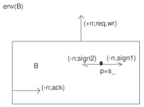
Figure 1. A typical block

$\sf{\partial(env(B))}$

2.2. Main Theorem

Definition 2.5.

For each message (i.e. input, output, sink/source) we define a measure $\mu$ – the information pressure – according to:

$$\begin{array}[]{l}\mu(i)=\mu(\mathbf{n};s_{1},...,s_{k})=k;\\ \mu(o)=\mu(-\,\mathbf{n};s_{1},...,s_{l})=-l;\\ \mu(s_{i})=\mu(\mathbf{n};s_{1},...,s_{p})=p\,;\\ \mu(s_{o})=\mu(-\,\mathbf{n};s_{1},...,s_{q})=-q\,.\end{array}$$

Remark 2.6.

Again, we allow the existence of ”mixed” punctures. In this case the measure associated which such a puncture is the arithmetic sum of its signals, considered with sign ”$+$” if they relate to a output, and with a ”$-$” if they correspond to an input.

Example 2.7.

Consider the puncture $p$ with messages: $(+\,{\bf n}\,;s_{1},s_{2}),\;(+\,{\bf n}\,;s_{3})\,,\;\\ (+\,{\bf n}\,;s_{4},s_{5})$. Then: $\mu(p)=2+1-2=1$.

With these notations we are in a position to formulate Green’s theorem for blocks:

Theorem 2.8.

Let $B$ be a block of(with) outputs $o(B)$, inputs $i(B)$ and sink/sources $p(B)=p_{+}(B)+p_{-}(B)$, where $p(B)$ denotes the set of punctures of the block $B$. Then the following holds:

(2.1) $$\sum_{i\in i(B)}\mu(i)+\sum_{o\in o(B)}\mu(o)+\sum_{p\in p(B)}\mu(s)=0$$

Proof Given a block $B$, every input/output signal is uniquely identified with a point on the boundary $Fr(B)$ with a length element given by the measure $\mu$ of the signal. Since overall-time information is conserved, applying Grenn’s Formula on such a block gives:

(2.2) $$0=\oint_{\partial(B)}{\footnotesize information}\,d\mu=\sum_{i\in i(B)}\mu(i)+\sum_{o\in o(B)}\mu(o)+\sum_{p\in p(B)}\mu(s)$$

$\Box$

Example 2.9.

The following simple rule relative to the block of Example 2.4 illustrates the method of implementing Formula  2.1:

$${\bf AG}\,({\tt(\neg ack\wedge req\wedge wr)}\rightarrow{\bf AF}\,{\tt ack})\qquad\rho$$

Since ${\tt req}$ and ${\tt wr}$ are outputs, they both contribute with a ”$+1$”, while ${\tt ack}$, being an input, adds a ”$-1$” to the general balance, so the measure variance associated to the rule $\varrho$ is $\Delta(\varrho)=1+1-1=1$. Note that - as stated before - we count only the asserted signals.
We shall show in Section 3 how to add the variances of individual rules in order to get the global variance $\Delta(B)$.

Note   Formula  2.1 should be understood as a qualitative indicator for the coverage of a given set of rules, hence this set is assumed to satisfy the following postulates:

1. Every input/output appears at least once in the set of rules, otherwise one could have, for instance the following set of rules, which consists of only one formula:

   $$\mathcal{S}_{1}\!:\;{\bf AG}\,({\tt req}\rightarrow{\bf AX}\,{\tt ack})\qquad\rho_{1}$$

   which satisfies  2.1, but evidently will not represent a complete set of rules for a realistic arbiter.

2. If a set of rules does not satisfy  2.1, it is guaranteed to be either incomplete or to have redundancies. On the other hand, sets of rules may satisfy  2.1, but still be inconsistent, such as the following:

   $$\mathcal{S}_{2}\!:\;\left\{\begin{array}[]{ll}{\bf AG}\,({\tt req}\rightarrow{\bf AX}\,{\tt ack})&\qquad\rho_{1}\\ {\bf AG}\,({\tt req}\rightarrow{\bf AX\,AX}\,{\tt ack})&\qquad\rho_{2}\end{array}\right.$$

   Indeed, if ”ack” is - as it normally does - a ”pulse” signal, then $\rho_{1}$ and $\rho_{2}$ will not be always satisfied in tandem by any normal system.
   Also, the following system contains a redundant rule:

   $$\mathcal{S}_{3}\!:\;\left\{\begin{array}[]{ll}{\bf AG}\,({\tt req}\rightarrow{\bf AX}\,{\tt ack})&\qquad\rho_{1}\\ {\bf AG}\,({\tt req}\rightarrow{\bf AF}\,{\tt ack})&\qquad\rho_{3}\end{array}\right.$$

   since if $\rho_{1}$ holds, then $\varrho_{3}$ is obviously redundant. However it still obviously satisfies  2.1, so a direct application of Theorem  2.8 will not reveal this fact.
   Therefore, it is imperative that the formalist satisfies the following:
   
   Fairness Assumption  The set of rules consists only of relevant rules and does                         not contain deliberate redundancies.

Remark 2.10.

Although, as shown in the previous Note, the given method does not give a completely automatic tool to solve the coverage problem, it gives the user, especially the skilled verifier, a numerical assessment of the block’s complexity. Two important conclusions ensue from this:
On one hand, a well formulated set of rules enables one to actually compute the complexity of the internal structure of the block, as this is expressed by the pressures contributed by the punctures, thus allowing a paradigm shift from the black-box concept to that of semi-transparent blocks.
On the other hand, it gives the verifier of neighboring blocks a computational tool for checking relative correctness along the common interface. This advantage becomes even more effective in pipelining units, for which the boundary interface is the simplest possible.

3. Case Studies

This work was partially motivated by the work of Katz, Grumberg and Geist (see [KGG]). We will demonstrate the application of  2.1 to the examples given in the paper mentioned above, and compare the results obtained and the efficiency of both methods.
Their main example consists of a synchronous arbiter $A$ having two inputs: ${\tt req1}$ and ${\tt req2}$ and two outputs: ${\tt ack1}$ and ${\tt ack2}$ (see Fig. 2).

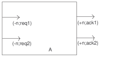
Figure 2. Arbiter

This arbiter’s behavior is (cf. [KGG] ) is described by the following complete set of rules that contains no redundancies:

$$\mathcal{S}:\left\{\begin{array}[]{ll}{\bf AG}\,[(\neg{\tt req1}\wedge\neg{\tt req2})\rightarrow{\bf AX}(\neg{\tt ack1}\wedge\neg{\tt ack2})]&\qquad\rho_{1}\\ {\bf AG}\,[({\tt req1}\wedge\neg{\tt req2})\rightarrow{\bf AX}{\tt ack1}]&\qquad\rho_{2}\\ {\bf AG}\,(\neg{\tt req1}\wedge{\tt req2})\rightarrow{\bf AX}{\tt ack2}]&\qquad\rho_{3}\\ {\bf AG}\,[({\tt req1}\wedge{\tt ack2})\rightarrow{\bf AX}{\tt ack1}]&\qquad\rho_{4}\\ {\bf AG}\,[({\tt req2}\wedge{\tt ack1})\rightarrow{\bf AX}{\tt ack2}]&\qquad\rho_{5}\\ {\bf A}\,[(\neg{\tt req1}\vee\neg{\tt req2}\vee{\tt ack1}\vee{\tt ack2}){\bf W}({\tt req1}\wedge{\tt req2}\wedge\neg{\tt ack1}\wedge\neg{\tt ack2}\wedge{\bf AX}{\tt ack1})]&\qquad\rho_{6}\\ ({\tt req1}\wedge{\tt req2}\wedge\neg{\tt ack1}\wedge\neg{\tt ack2})\rightarrow{\bf AX}[{\tt ack1}\rightarrow\\ {\bf A}\,[(\neg{\tt req1}\vee\neg{\tt req2}\vee{\tt ack1}\vee{\tt ack2}){\bf W}({\tt req1}\wedge{\tt req2}\wedge\neg{\tt ack1}\wedge\neg{\tt ack2}\wedge{\bf AX}{\tt ack2})]]&\qquad\rho_{7}\\ ({\tt req1}\wedge{\tt req2}\wedge\neg{\tt ack1}\wedge\neg{\tt ack2})\rightarrow{\bf AX}[{\tt ack2}\rightarrow\\ {\bf A}\,[(\neg{\tt req1}\vee\neg{\tt req2}\vee{\tt ack1}\vee{\tt ack2}){\bf W}({\tt req1}\wedge{\tt req2}\wedge\neg{\tt ack1}\wedge\neg{\tt ack2}\wedge{\bf AX}{\tt ack1})]]&\qquad\rho_{8}\\ \end{array}\right.$$

The computation of the variances for the rules above is summarized in the table bellow:

	Message Type
Rule	Input(s)		Output(s)		$\Delta$
	req1	req2	ack1	ack2
$\rho_{1}$	0	0	0	0	0
$\rho_{2}$	1	0	1	0	0
$\rho_{3}$	0	1	0	1	0
$\rho_{4}$	1	0	1	1	+1
$\rho_{5}$	0	1	1	1	+1
$\rho_{6}$	1	1	2	1	+1
$\rho_{7}$	2	2	2	2	0
$\rho_{8}$	2	2	2	2	0

Figure 3.

Then $\Delta(A)=\Delta(\rho_{1})+...+\Delta(\rho_{8})=+3$. That is:

$$\sum_{i\in i(A)}\mu(i)+\sum_{o\in o(A)}\mu(o)=+3\neq 0.$$

Thus, in order for  2.1 to hold, the arbiter also must have a puncture, responsible resulting from the logical complexity of the block.
Indeed, expressed in the $SMV$ language, the inner structure of the arbiter is given (again cf. [KGG] ) by:

$$\begin{array}[]{ll }var\\ \quad req1,req2,ack1,ack2,robin:boolean;\\ assign\\ \quad init(ack1):=0;\\ \quad init(ack2):=0;\\ \quad init(robin):=0;\\ next(ack1):=case\\ \quad!req1\qquad:0;\\ \quad!req2\qquad:1;\\ \quad!ack1\,\&\,!ack2\qquad:\,!robin;\\ \quad 1\qquad:!ack1;\\ esac;\\ next(ack2):=case\\ \quad!req2\qquad:0;\\ \quad!req1\qquad:1;\\ \quad!ack1\,\&\,!ack2\qquad:\,robin;\\ \quad 1\qquad:!ack1;\\ esac;\\ next(robin):=if\>req1\,\&\,req2\,\&\,!ack1\,\&\,!ack2\;\;then\;\,!robin\\ \qquad\qquad\qquad\quad\ else\>\,robin\>\,endif;\end{array}$$

Therefore, a more realistic representation of the arbiter would be given by Fig.4:

Figure 4. An Improved Arbiter

Since ”robin” is asserted iff ”ack1” or ”ack2” are asserted, the signal ”robin” will appear three times and, since it is emitted by the puncture towards the arbiter, its sign will be ”-”. Thus $\sum_{p\in p(A)}\mu(s)=-3$, as required and, indeed, the fact that the system $\mathcal{S}$ is complete and contains no redundancies is expressed by the fact that the variance we have found ($\Delta$ = 3) exactly balances with the contribution of the internal logic due to the ”robin” puncture.
We further test our method by applying it on the same variations of the main example as considered in [KGG] and concisely comparing the results.
The first variation is produced by replacing rule $\rho_{4}$ by $\rho_{4}^{\prime}$, thus considering the modified system $\mathcal{S^{\prime}}$, and also modifying the internal structure of the arbiter by inserting the new lines bellow: (Here and in the following examples the new/modified rules appear in bold characters.)

$$\mathcal{S^{\prime}}:\left\{\begin{array}[]{ll}{\bf AG}\,[(\neg{\tt req1}\wedge\neg{\tt req2})\rightarrow{\bf AX}(\neg{\tt ack1}\wedge\neg{\tt ack2})]&\qquad\rho_{1}\\ {\bf AG}\,[({\tt req1}\wedge\neg{\tt req2})\rightarrow{\bf AX}{\tt ack1}]&\qquad\rho_{2}\\ {\bf AG}\,(\neg{\tt req1}\wedge{\tt req2})\rightarrow{\bf AX}{\tt ack2}]&\qquad\rho_{3}\\ {\bf AG}\,[({\tt req1}\wedge{\tt ack2})\rightarrow{\bf AX}({\tt ack1\vee ack2})]&\qquad\huge{\mathbf{\rho_{4}^{\prime}}}\\ {\bf AG}\,[({\tt req2}\wedge{\tt ack1})\rightarrow{\bf AX}{\tt ack2}]&\qquad\rho_{5}\\ {\bf A}\,[(\neg{\tt req1}\vee\neg{\tt req2}\vee{\tt ack1}\vee{\tt ack2}){\bf W}({\tt req1}\wedge{\tt req2}\wedge\neg{\tt ack1}\wedge\neg{\tt ack2}\wedge{\bf AX}{\tt ack1})]&\qquad\rho_{6}\\ ({\tt req1}\wedge{\tt req2}\wedge\neg{\tt ack1}\wedge\neg{\tt ack2})\rightarrow{\bf AX}[{\tt ack1}\rightarrow\\ {\bf A}\,[(\neg{\tt req1}\vee\neg{\tt req2}\vee{\tt ack1}\vee{\tt ack2}){\bf W}({\tt req1}\wedge{\tt req2}\wedge\neg{\tt ack1}\wedge\neg{\tt ack2}\wedge{\bf AX}{\tt ack2})]]&\qquad\rho_{7}\\ ({\tt req1}\wedge{\tt req2}\wedge\neg{\tt ack1}\wedge\neg{\tt ack2})\rightarrow{\bf AX}[{\tt ack2}\rightarrow\\ {\bf A}\,[(\neg{\tt req1}\vee\neg{\tt req2}\vee{\tt ack1}\vee{\tt ack2}){\bf W}({\tt req1}\wedge{\tt req2}\wedge\neg{\tt ack1}\wedge\neg{\tt ack2}\wedge{\bf AX}{\tt ack1})]]&\qquad\rho_{8}\\ \end{array}\right.$$

$$\begin{array}[]{ll }var\\ \quad req1,req2,ack1,ack2,robin:boolean;\\ assign\\ \quad init(ack1):=0;\\ \quad init(ack2):=0;\\ \quad init(robin):=0;\\ next(ack1):=case\\ \quad!req1\qquad:0;\\ \quad!req2\qquad:1;\\ \quad!ack1\,\&\,!ack2\qquad:\,!robin;\\ \quad\mathbf{robin\,\&\,ack2\qquad:\{0,1\};}\\ \quad 1\qquad:!ack1;\\ esac;\\ next(ack2):=case\\ \quad!req2\qquad:0;\\ \quad!req1\qquad:1;\\ \quad!ack1\,\&\,!ack2\qquad:\,robin;\\ \quad\mathbf{ack2\qquad:!next(ack1);}\\ \quad 1\qquad:!ack1;\\ esac;\\ next(robin):=if\>req1\,\&\,req2\,\&\,!ack1\,\&\,!ack2\;\;then\;\,!robin\\ \qquad\qquad\qquad\quad\ else\>\,robin\>\,endif;\end{array}$$

These changes produce a positive overall variance $\Delta(A^{\prime})=3>0$; thus indicating the unbalance introduced due to redundancy the System of Laws fitting, to the ”Unimplemented Transition Evidence” considered in [KGG]). The next example relates to the so called ”Unimplemented State Evidence” of [KGG]. It is produced by introducing an internal auxiliary variable of ”input” type , thus augumenting the internal complexity of the arbiter, in a way that can not be detected and balanced by the rules. In this case the modifications bellow indeed generate a negative $\Delta(A^{\prime\prime})$, as expected.

$$\begin{array}[]{ll}var\\ \quad\mathbf{req1_{-}temp,req2,ack1,ack2,robin:boolean;}\\ \mathbf{define\;req1:=req1_{-}temp\,\&\,!(ack1\,\&\,ack2);}\\ assign\\ \quad init(ack1):=0;\\ \quad init(ack2):=0;\\ \quad init(robin):=0;\\ next(ack1):=case\\ \quad!req1\qquad:0;\\ \quad!req2\qquad:1;\\ \quad!ack1\,\&\,!ack2\qquad:\,!robin;\\ \quad\mathbf{ack1\qquad:\{0,1\};}\\ \quad 1\qquad:!ack1;\\ esac;\\ next(ack2):=case\\ \quad!req2\qquad:0;\\ \quad!req1\qquad:1;\\ \quad!ack1\,\&\,!ack2\qquad:\,robin;\\ \quad 1\qquad:!ack1;\\ esac;\\ next(robin):=if\>req1\,\&\,req2\,\&\,!ack1\,\&\,!ack2\;\;then\;\,!robin\\ \qquad\qquad\qquad\quad\ else\>\,robin\>\,endif;\end{array}$$

Finally, we consider the modification bellow:

$$\begin{array}[]{ll }var\\ \quad\mathbf{req1,req2,req11,req21,ack1,ack2,ack11,ack21,robin:boolean;}\\ assign\\ \quad\mathbf{init(ack1):=0;\;init(ack11):=0;}\\ \quad\mathbf{init(ack2):=0;\;init(ack21):=0;}\\ \quad init(robin):=0;\\ \mathbf{define}\\ \mathbf{ack1:=case}\\ \mathbf{\quad!req11\qquad:0;}\\ \mathbf{\quad!req21\qquad:1;}\\ \mathbf{\quad!ack11\,\&\,!ack21\qquad:\,!robin;}\\ \mathbf{\quad 1\qquad:!ack11;}\\ esac;\\ next(ack2):=case\\ \mathbf{\quad!req21\qquad:0;}\\ \mathbf{\quad!req11\qquad:1;}\\ \mathbf{\quad!ack11\,\&\,!ack21\qquad:\,robin;}\\ \mathbf{\quad 1\qquad:!ack11;}\\ esac;\\ next(robin):=if\>req1\,\&\,req2\,\&\,!ack1\,\&\,!ack2\;\;then\;\,!robin\\ \qquad\qquad\qquad\quad\ else\>\,robin\>\,endif;\\ \mathbf{next(req11):=req1;\;next(req21):=req2};\\ \mathbf{next(ack11):=ack1;\;next(ack21):=ack2};\end{array}$$

Since it is basically produced by multiplying the true original signals, the resulting $\Delta(A^{\prime\prime\prime})$ is a indeed a multiple of the original (corresponding to the ”Many to One” (cf. [KGG]).

Remark 3.1.

While the existence of punctures is remarked in [KGG] (the so-called ”Non-Observable Implementation Variables”), the approach described in the mentioned article can not detect them. This emphasizes one of the strengths of the method proposed here: it not only detects the above mentioned punctures, but it also estimates them numerically.

4. Global Theory

Since the coverage problem is more crucial in large scale systems, i.e. for units composed of several blocks, it is natural to try to extend the method presented here to such systems as well.
This is possible in the same way that Green’s Theorem extends from simply-connected regions to multiply connected regions. In this manner we obtain the following:

Proposition 4.1.

Let $U$ be a unit with bounded environment components $B_{j}$, each of which corresponds to some block component of $U$. For each $B_{j}$ let $\Delta_{i}$ denote the difference $\Delta_{i}=\sum_{i\in i(B_{j})}\mu(i)-\sum_{o\in o(B_{j})}\mu(o)$.
Then $U$ satisfies:

(4.1) $$\sum_{j}\mu_{U}(i)-\sum_{j}\mu_{U}(o)+\sum_{j}\Delta_{j}=0$$

where $\mu_{U}(i),\mu_{U}(o)$ are the information measures of $U$ w.r.t. its external environment component. In short, if we denote $\Delta U=\sum_{j}\mu_{U}(i)-\sum_{j}\mu_{U}(o)$, then the following holds:

(4.2) $$\Delta(U)=-\sum_{j}\Delta_{j}$$

Example 4.2.

The example described in Fig. 5 represents schematically the control unit of a A Bus Interface Unit (cf. [GLS] ) and its component blocks.

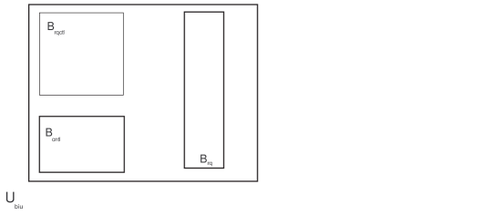
Figure 5. The Control unit of a Bus Interface Unit (following [GLS])

Then $\Delta(U_{biu})=-\big{(}\,\Delta(B_{cntl})+\Delta(B_{rq})+\Delta(B_{rqctl})\big{)}$

Given the technique above, it is evident how to proceed ”upward” for larger and larger units: we consider an integrated circuit $S$ as top level $S=S_{0}=L_{0}$, its composing units as the first level $L_{1}=\{S_{1,m}\}$, their structural subunits as the 2-nd level $L_{2}=\{S_{2,n}\}$, and so on, where, at the ”$k$”-th level ”$S_{k}$” denote the elementary blocks, so eventually we have the following generalization of Theorem 2.8:

Theorem 4.3.

(4.3) $$\Delta(S)=\Delta(S_{0})=-\sum\Delta(S_{1})=\sum\sum(\Delta(S_{2}))=\ldots=(-1)^{k}\underbrace{\sum\cdots\sum}_{k\,sums}\Delta(S_{k})$$

Example 4.4.

The example presented in Fig. 6 shows a A Bus Interface Unit (cf. [GLS] ). The whole Processor $S$ is designated as level 0 ($L_{0}$ ), the $BIU$ $U_{biu}$ being one of he components of level 1 ($L_{1}$). The drawing(scheme) also shows the building blocks of $U_{biu}$, which belong to Level 2 ($L_{2}$).

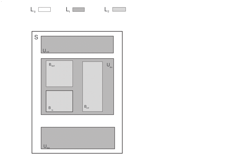
Figure 6. A Bus Interface Unit (after [GLS])

Remark 4.5.

Theorem 4.3. gives the verifier the ability to encompass a global estimate viewpoint of the complexity of a large system, ”from top to bottom”, as the formula can be readily used at the architectural stage, through the design faze, down to the verification stage where. At each stage the more complex units are being characterized by having large pressure contributions. Thus permitting the immediate extension of Model Checking methods to very large scale systems in a manner which is point-wise precise.

5. Future Work

Since punctures, blocks, units, etc., display the same arithmetic behavior, it is only natural to regard each component at any given level as a puncture of the unit of the component containing it and which belongs to next upper level. Therefore it appears that the appropriate and promising way to study the intrinsic nature of integrated circuits would be by means of Networks and Graph Theory. Such study is currently in progress.

6. Appendix

Theorem 6.1.

(Green) Let $S=int(S)\subseteq\mathbb{R}^{2}$ be an open set in the plane and let $P,Q:U=int(S)\rightarrow\mathbb{R}^{2}$ continuously differentiable functions. Let $\gamma\subset S$ be a piecewise smooth simple, closed curve, and let $R=int(\gamma)$ (i.e. $c=\partial{R}$).
Then:

(6.1) $$\int\int_{\footnotesize R}\Big{(}\frac{\partial{Q}}{\partial{x}}-\frac{\partial{P}}{\partial{y}}\Big{)}dxdy=\oint_{\partial{R}}Pdx+Qdy$$

In vectorial notation (6.1) has the following form:

(6.2) $$\int\int_{\footnotesize R}div\,\overrightarrow{V}dxdy=\oint_{\partial{R}}\overrightarrow{V}\cdot\overrightarrow{n}ds$$

where $\overrightarrow{V}=(Q,-P)$, $div\,\overrightarrow{V}=\frac{\partial{Q}}{\partial{x}}-\frac{\partial{P}}{\partial{y}}$ is the divergence of the vector field $\overrightarrow{V}$, $\overrightarrow{n}=+\,\bf{n}$ is the unit outer normal to $\partial{R}$, and $ds$ represents the length element of $\partial{R}$.
The classical interpretation of (6.2) above is the following: $\overrightarrow{V}$ represents the flux density of an incompressible fluid, then $div\overrightarrow{V}$ measures the amount of mass transported away from each point per time unit. This quantity differs from zero only then there are sinks and/or sources. Thus $\int\int_{\footnotesize R}div\overrightarrow{V}dxdy$ measures the amount of fluid escaping from (respectively entering) the region $R$ through $\partial{R}$. Therefore (6.2) expresses the Mass Conservation Law for $R$.

References

- [CGP] Clarke,E.M. Jr. , Grumberg, O. and Peled D.A. Model Checking , The MIT Press, 1999.
- [GLS] Geist, D. Landver, A. and Singer, B.W. Formal Verification of a Processor’s Bus Interface Unit , IBM Technical Report, 1996.
- [KGG] Katz, S. , Grumberg, O. and Geist, D. ”Have I written enough proprieties?” - A method of comparison between specification and implementation , CHARME’99, Bad Herrenalb, Germany, September 27-29, 1999.
- [McM] McMillan, K.L. Symbolic Model Checking , Kluwer Academic Publishers, 1993.
- [P] Parash, A. Formal Verification of an MPEG Decoder Chip: A case study in the industrial use of formal methods , WAVe 2000 - a CAV’2000 workshop.
- [AS] Apelboim, E. and Saucan, E. The Axiomatic Approach to Model Checking in preparation.
- [HKHZ] Hoskote, Y. Kam, T. Ho, P.-S. and Zhao, X. Coverage Estimation for Symbolic Model Checking , In ”Proceedings of the 36-rd Design Automation Conference (DAC’99)”, IEEE Computer Society Press, June 1999.
- [A] Apostol, Tom M. , Calculus, volume II, Blaisdell, New York,third edition, 1965.