Controlled hierarchical filtering: Model of neocortical sensory processing

Abstract.

A model of sensory information processing is presented. The model assumes that learning of internal (hidden) generative models, which can predict the future and evaluate the precision of that prediction, is of central importance for information extraction. Furthermore, the model makes a bridge to goal-oriented systems and builds upon the structural similarity between the architecture of a robust controller and that of the hippocampal entorhinal loop. This generative control architecture is mapped to the neocortex and to the hippocampal entorhinal loop. Implicit memory phenomena; priming and prototype learning are emerging features of the model. Mathematical theorems ensure stability and attractive learning properties of the architecture. Connections to reinforcement learning are also established: both the control network, and the network with a hidden model converge to (near) optimal policy under suitable conditions. Falsifying predictions, including the role of the feedback connections between neocortical areas are made.

1. Introduction

Our thinking is best expressed by the words of Albert Szent-Györgyi [125], the famous Hungarian Nobel Laureate: ‘There is no real difference between structure and function; they are the two sides of the same coin. If structure does not tell us anything about function, it means we have not looked at it correctly.’

Here, a general framework is searched for that explains information processing function of the brain, extends to the goal-oriented nature of information processing and explains the structure given these functions. For the sake of clarity, first our assumptions about the function shall be stated. Built on the assumptions, we shall work on ‘deriving’ the building blocks of structure. Finally, these blocks will be mapped to the substrate.

1.1. Starting assumptions

The model is built on a few interlinked ‘axioms’:

1. The brain interacts with the environment, signals are received and responses are generated.

2. Signal detection corresponds to filtering of all possible detectable phenomena.

3. Response generation influences the environment, influence on the environment is goal oriented and aims to control environmental parameters.

4. Control of the environment is subject to optimization.

1.2. ‘Guiding principles’

Our starting assumptions are constrained as follows:

The homunculus fallacy should be solved

Our thoughts are grounded on the hypothesis that representations do exist in the brain (see e.g. the debates about the Representational Theory of Mind and its modern extension, the Computational Theory of Mind [25, 17], but also [19]). The use of representations can hardly be avoided in any computational modelling. Generally speaking, the processing of signals that may convey information can be considered as a transformation into another form that still carries the whole amount or just a piece of the original information. The environment feeds the system with some inputs and the system output represents (a part of) the environment. Whilst most models address the problem of coding inputs and making efficient internal representation, we are more concerned about the fundamental problem of making sense of these representations. In our view, the central issue of making sense or meaning is to provide answers to questions like ‘what does it mean?’ in terms of our past experiences, or ‘how are they related?’ in terms of known facts. In other words, making sense is inherently related to declarative memory. As a consequence, the homunculus fallacy (see e.g., [116]) — that the internal representation is meaningless without an interpreter — is of central importance. This fallacy claims that all levels of abstraction require at least one further level to become the corresponding interpreter. Unfortunately, the interpretation — according to the fallacy — is just a new transformation and we are trapped in an endless regression.

1.2.1. Constraint of reconstruction

Our standpoint is that the paradox stems from vaguely described procedure of ‘making sense’. The fallacy arises by saying that the internal representation should make sense. One can turn the fallacy upside down by changing the roles [73]: Not the internal representation but the input should make sense. Our proposal is that the input makes sense if the same (or similar) inputs have been experienced before and if the input can be derived or regenerated by means of the internal representation [73, 81]. All in all, the goal is to turn the infinite regression into a reconstructing loop structure and shortcut the fallacy. According to this approach the internal representation interprets the input by (re)constructing it. This function is more than mirroring the environment. Interpretation based reconstruction can fill in missing parts of spatio-temporal patterns, which includes the capacity of prediction.

1.2.2. Constraints of control and optimization

Interpretation is goal oriented and forms a delicate

‘perception-action loop’: The actual goal requires (1) the sensing of environmental parameters, (2) the ability to influence, i.e, to control those parameters, (3) the sensing of consequences of control and so on. In turn, perceptual information is transformed, transformation is controlled and the control of transformation is subject to the actual goal. Because transformation depends on the actual goal, control typically acts on a partially observed environment; information is filtered.

Sensing and control of the environment consumes energy, which should be minimized. Minimization of energy consumption is a long-term task: short term saving at the cost of large long-term spending needs to be avoided and long-term cumulated cost is to be minimized. Such optimization problems are formulated within the framework of reinforcement learning (RL). It is then necessary to consider control concepts subject to principles developed in RL in partially observed environments. This challenging [84] and generally computationally intractable problem [15, 71] should be addressed by the model.

1.2.3. Architectural constraints on the neural level

There are constraints on the building blocks of the filtering and controlling system, such as

1. Locality: The architecture is made of connected simple computational units. Connected units are neighbors. Computations of any unit are based on information received from its neighbors.

2. Connections are directed and serve as filters. Connections possess tunable filtering strength or weights. Tuning of connections is subject to Hebbian-learning: signals of the two computational units at the two ends of a directed connection determine the adaptation of the weight of the connection.

3. Locality and Hebbian-learning concern all functions, including sensing, control and optimization.

1.2.4. Anatomical constraints

The architecture should match known architectural properties of sensory processing areas of the neocortex up to the top, the hippocampus (HC) and its surrounding, the hippocampal formation.

1.3. Origins of the model

Ever since the discovery of the central role of the hippocampus and its adjacent areas in memory formation [117, 88], numerous studies and models dealt with the properties and the possible functions of the hippocampus and its environment. The number of new experimental findings is increasing and highlight the complexity of the behavior of memory. Although views are strikingly different, they seem to have their own, experimentally supported merits. The interested reader is referred to the literature for excellent reviews on the hippocampus written, e.g., by Squire [121], Hasselmo and McClelland [41], Redish [106] and O’Reilly and Rudy [97]. The majority of the models have been developed to describe one part (mainly the CA3 field) of the hippocampus (see, e.g. [69, 56]). Attempts have been made to develop an integrating model of the HC [108, 43, 70, 24, 42]. See also works collected by Gluck [27]. It is known though, that hippocampus is deeply embedded in the neocortical information flow through the entorhinal cortex (EC).

This fact explains the emergence of a few EC-HC models like [86, 89, 75, 109, 80, 96]. For example, McClelland et al. [86] emphasize the necessity of a dual system for the seemingly contradictory tasks of learning of specific properties and allowing for generalization.

The controlled hierarchical filtering (CHF) model that we present here, has its origin in the old standing proposal that the hippocampus and/or its environment serve as a ‘comparator’ [32, 120, 139]. More recent works about this subject try to provide a neuro-psychological account of anxiety and consciousness [33, 34, 36, 35]. Other models use somewhat different nomenclature, e.g., the focus is placed on match/mismatch detection [102, 93, 37]. Match/mismatch detection is closely related to familarity/novelty detection, another direction of theoretical efforts to describe medial temporal lobe areas [98, 110, 141]. The form of novelty is probably polymorphous and there is increasing evidence that different brain areas share the task of recognizing different aspects of novelty within the same scene [140]. It seems that the encoding of novelty is distributed, which is a crucial point of the CHF model.

The CHF architecture is an extension of our previous works [75, 76, 80]. It may be worth noting that two falsifying predictions of that model, (a) large and tunable temporal delaying capabilities of neurons of the dentate gyrus and (b) persistent activities at deep layers of the entorhinal cortex have been reinforced recently by Henze et al., [44] and by Egorov et al. [23], respectively.

The paper is constructed as follows. First (in Section 2), terminology is provided and basic concepts are defined. The CHF model is detailed here. Section 3 deals with the mapping of the control and

reconstruction architectures to the entorhinal-hippocampal loop and to neocortical areas. Section 4 discusses relations to other computational models, e.g.,

[29, 122, 104, 105, 9]. This section treats learning and stability properties of the architecture, connections between RL and the model architecture, connections to RL and to partially observed RL problems, the emerging neurobiological features, missing links and some conjectures of the model. The paper is finished by an Appendix containing some of the mathematical details. Other mathematical details can be found in the cited references, including the technicalities, which are made available as technical reports through http://arxiv.org.

2. Model construction

Notations of the control field and notations of neuron networks differ. In control theory, input-output systems are considered. In graphical form, box denotes the system and arrows denote the system’s input(s) and output(s). Processing occurs in the box (Fig. 1(A)). On the contrary, artificial neural networks consist of computational units, the putative analogs of real neurons. The units, also called neurons, receive (provide) inputs (outputs) through the connection structure, and this internal functioning is drawn explicitly. Neurons execute simple computations, like summing up inputs, thresholding and alike. The main part of the neural network performs distributed computation using the connection structure performing (non-linear) filtering. This distributed filter system, which may connect all neurons, is called the connection system, weights, or synapses. In a neural network architecture different neural layers are distinguished. Connections between these layers are explicitly drawn in most cases (Fig. 1(B)). Computations of neural networks between their inputs and outputs can be given in the following condensed form:

(1) $$\mathbf{y}=f(\mathbf{Wx})$$

where input and output are denoted by $\mathbf{x}\in\mathbb{R}^{n}$ and $\mathbf{y}\in\mathbb{R}^{m}$, respectively, linear transformation from $\mathbb{R}^{n}$ to $\mathbb{R}^{m}$ is represented by matrix $\mathbf{W}\in\mathbb{R}^{m\times n}$, the connections, and function $f$ denotes components-wise non-linearity. If this function is the identity function, then we have a linear network. Here, a simplified notation will be used: neural layers will be denoted by horizontal thick lines. Any particular set of connections between two layers will be represented by a single arrow. A feedforward linear network is depicted in Fig. 1(C). The graphical form of a network with component-wise non-linearity is shown in Fig. 1(D). Different transformations may exist between two layers. Recurrent connections (also called ‘recurrent collaterals’) target the same layer where they originate from.

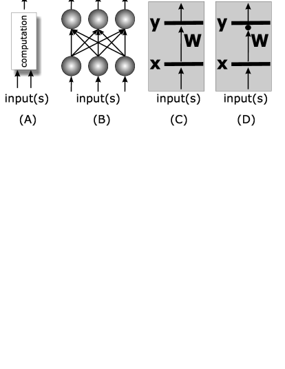
Figure 1. Notations
A: Control representation of input output systems. Computations are performed in the box.
B: Neural network representation of computations: inputs are received by input neurons and are (non-linearly) transformed by connections and the output neurons, which provide the outputs. An output neuron could be an input neuron of the next processing stage.
C: Linear neural transformation. Input: $\mathbf{x}$, transformation $\mathbf{W}$, output: $\mathbf{y}$, $\mathbf{y}=\mathbf{W}\mathbf{x}$.
D: Non-linear neural transformation. $\mathbf{y}=f(\mathbf{W}\mathbf{x})$. Graphical form: arrow with a circle. More than one transformation may exist between layers. Recurrent network is a neural layer with a transformation that targets the same layer.
Terminology in the context of neurobiology:
Layer corresponds to a given area sometimes called field or subfield, such as the CA3 and CA1 regions of the hippocampus, or the different layers of the neocortex. Transformations may correspond to (i) excitatory synapses connecting layers or targeting neurons of the same layer, such as the recurrent collaterals and the associative connections of the CA3 subfield of the hippocampus and the intra-layer excitatory connections of layers II and III of the neocortex or (ii) inhibitory synapses between layers or within layers, such as the rich interneural networks in the hippocampus.

2.1. The control model

Our control problem is formulated in terms of state dependent directions pointing towards target positions. A mapping which renders direction (change of state, or change of state per unit time, i.e., velocity) to each state is called speed-field. A particular speed-field is given, for example, by the difference vectors between the target state and all other states. An important feature of speed-field is that motion is not specified in time. The control task is defined as moving according to the speed-field at each state. This control task is called speed-field tracking (SFT). For a review on SFT, see, e.g., [49]. SFT formulation is flexible because different fields can be designed for the same task and, also, it allows motions to speed up or to slow down simply by scaling of the speed-field. Speed-field can be seen as a local tool for path planning (see, e.g., [26] and references therein). The control task of path (also called trajectory) tracking is, however, different. The difference between SFT and ordinary trajectory tracking is shown in Fig. 2. One might say that SFT is less stringent, less precise and puts more emphasis on the global goal than on the local perturbations.

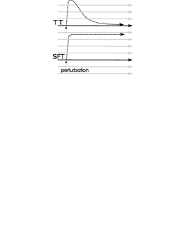
Figure 2. Trajectory tracking (TT) versus speed field tracking (SFT)
TT: Horizontal lines represent different nearby trajectories. Black line: initial trajectory. Upon perturbations the system (the ‘plant’) should return to the original trajectory.
SFT: Horizontal lines represent a small part of the speed-field to be tracked. Black line: initial speed trajectory. Upon perturbation, the plant adjusts its speed to the speed of the actual neighborhood.

The dynamic equation of a system is a (possibly continuous) set of differential equations. This set of equations determines the change of state per unit time given the external forces acting upon the system, including the control action. Inverse dynamics works in the opposite way: given the state and (desired) change of state, inverse dynamics provides the control vector. If the inverse dynamics is perfect then inserting the control vector into the dynamic equation the desired change of state is achieved. The controller, in turn, maps state and speed to control action.

Inverse dynamics, however, changes if kinematic parameters (such as dimensions; length, width, etc.), or parameters of the dynamics (e.g., weight, flexibility and so on) change: Inverse dynamics is almost never perfect. Moreover, it is well known, that approximate inverse dynamics can give rise to instabilities [54]. In turn, a robust extension of speed-field tracking is needed. Such robust control architecture is described here.

Let $\mathbf{x}$ and $\mathbf{\dot{x}}$, where ‘dot’ denotes temporal derivation, represent the state and the change of the state per unit time (the momentum) of the plant, respectively. Let

(2) $$\mathbf{\dot{x}}=\mathbf{f}(\mathbf{x},\mathbf{u})$$

denote the dynamics of the plant, i.e., in state $\mathbf{x}\in\mathbb{R}^{n}$ and under control $\mathbf{u}\in\mathbb{R}^{p}$, the momentum of the plant becomes $\mathbf{\dot{x}}\in\mathbb{R}^{n}$ described by the nonlinear function $\mathbf{f}:\mathbb{R}^{n\times p}\rightarrow\mathbb{R}^{n}$. Let $\mathbf{v}(\mathbf{x})\in\mathbb{R}^{n}$ denote the desired change of state (the desired momentum). Assume that we have an approximate feedforward model of the inverse dynamics:

(3) $$\mathbf{u}_{ff}=\mathbf{u}_{ff}(\mathbf{x},\mathbf{\dot{x}},\mathbf{v}(\mathbf{x}))$$

which is an input-output system receiving inputs (the state, the momentum, the desired momentum) and providing output (the control vector $\mathbf{u}_{ff}:\mathbb{R}^{n\times n\times n}\rightarrow\mathbb{R}^{p}$). If this control vector is used directly to influence the plant then it is called feedforward controller. The perfect feedforward control vector $\mathbf{u}^{*}_{ff}$ makes the plant to produce momentum $\mathbf{v}(\mathbf{x})$:

(4) $$\mathbf{v}(\mathbf{x})=\mathbf{f}(\mathbf{x},\mathbf{u}^{*}_{ff}(\mathbf{x},\mathbf{\dot{x}},\mathbf{v}(\mathbf{x})))$$

If the feedforward control vector is imprecise then error (a difference between the desired momentum and the experienced momentum) $\mathbf{e}_{c}=\mathbf{v}(\mathbf{x})-\mathbf{\dot{x}}$ appears. To correct this error, the (same or another) model of the inverse dynamics can be used. This error correcting controller is called feedback controller: its inputs are the state, the momentum and the desired compensation, i.e., $\mathbf{e}_{c}$. The output of the feedback controller is subject to temporal integration. The output is called the feedback control vector $\mathbf{u}_{fb}$. The time integrated and amplified output of this controller is used to correct the feedforward control vector:

(5) $$\mathbf{\dot{w}}=\Lambda\mathbf{u}_{fb}$$

(6) $$\mathbf{u}=\mathbf{u}_{ff}+\mathbf{w}$$

i.e., $\mathbf{u}=\mathbf{u}_{ff}+\Lambda\int\mathbf{u}_{fb}\,dt$ where $\Lambda$ denotes the (amplifying) gain factor. Feedback vector $\mathbf{u}_{fb}$ disappears when $\mathbf{u}_{ff}=\mathbf{u}^{*}_{ff}$. Assume an approximate inverse dynamics of the following form:

(7) $$\mathbf{u}=\mathbf{\hat{\Phi}}(\mathbf{x},\mathbf{\dot{x}}).$$

A particular form of the feedback control vector is simply a comparator that disappears provided that $\mathbf{u}_{ff}(\mathbf{x},\mathbf{\dot{x}},\mathbf{v}(\mathbf{x}))$ is perfect:

(8) $$\mathbf{u}_{fb}=\mathbf{\hat{\Phi}}(\mathbf{x},\mathbf{v}(\mathbf{x}))-\mathbf{\hat{\Phi}}(\mathbf{x},\mathbf{\dot{x}})$$

This scheme is depicted in Fig. 3.

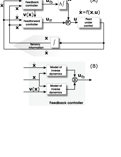
Figure 3. Robust controller for speed-field tracking tasks
A: The model of the inverse dynamics is inputted by the actual state $\mathbf{x}$, the momentum $\mathbf{\dot{x}}=\frac{d\mathbf{x}}{dt}$ , and the desired momentum at the actual state $\mathbf{v}(\mathbf{x})$. The output of the model is the feedforward control vector $\mathbf{u}_{ff}=\mathbf{u}_{ff}(\mathbf{x},\mathbf{\dot{x}},\mathbf{v}(\mathbf{x}))$. The feedforward control vector may need corrections. The feedback control vector, which is inputted by the state, the momentum and the desired compensation $\mathbf{e}_{c}=\mathbf{v}(\mathbf{x})-\mathbf{\dot{x}}$ serves this purpose. The output of the feedback controller is integrated by time, it is multiplied by the gain factor $\Lambda$ and the result is added to the feedforward control vector to form the approximate control vector $\mathbf{u}$.
B: The feedback controller is composed of two simplified models of the inverse dynamics. Their effect cancels and, in turn, feedback control action disappears when the feedforward controller is perfect, i.e., when control vector $\mathbf{u}_{ff}$ produces the desired momentum: $\mathbf{\dot{x}}=\mathbf{v}(\mathbf{x})$. These models have two arguments, the state and the momentum. The first model is inputted by the actual state and the desired momentum. The output of the model makes a positive contribution. The second model uses the actual state and the actual momentum. The difference of the two outputs, $\mathbf{u}_{fb}=\mathbf{\hat{\Phi}}(\mathbf{x},\mathbf{v}(\mathbf{x}))-\mathbf{\hat{\Phi}}(\mathbf{x},\mathbf{\dot{x}})$, is the feedback control vector.

2.2. From control architecture to reconstruction networks

Our control architecture can be related to a reconstruction network. To see this, first a particular (state dependent but linear) form of the inverse dynamics is assumed [128]:

(9) $$\mathbf{\hat{\Phi}}(\mathbf{x},\mathbf{\dot{x}})=\mathbf{\hat{A}}(\mathbf{x})\mathbf{\dot{x}}+\mathbf{b}(\mathbf{x}).$$

It has been shown that one can use the feedback controller in ‘feedforward position’ without effecting stability properties [128]:

(10) $$\mathbf{u}_{ff}=\mathbf{\hat{\Phi}}(\mathbf{x},\mathbf{v}(\mathbf{x}))-\mathbf{\hat{\Phi}}(\mathbf{x},\mathbf{\dot{x}})$$

In this case the feedforward controller will never be perfect. Explicit modelling of $\mathbf{b}(\mathbf{x})$, is unnecessary given that this quantity falls out in this comparation-based controller

(11) $$\mathbf{u}_{fb}(\mathbf{x},\mathbf{\dot{x}},\mathbf{v}(\mathbf{x}))=\mathbf{u}_{fb}(\mathbf{x},\mathbf{\dot{x}},\mathbf{v}(\mathbf{x}))=\mathbf{\hat{A}}(\mathbf{x})\left(\mathbf{v}(\mathbf{x})-\mathbf{\dot{x}}\right).$$

This simplified architecture, which is built of comparators is depicted in Fig. 4. We note that (i) the control scheme is capable of controlling plants of any order (Appendix 5.2) and (ii) it has attractive global stability properties [128].

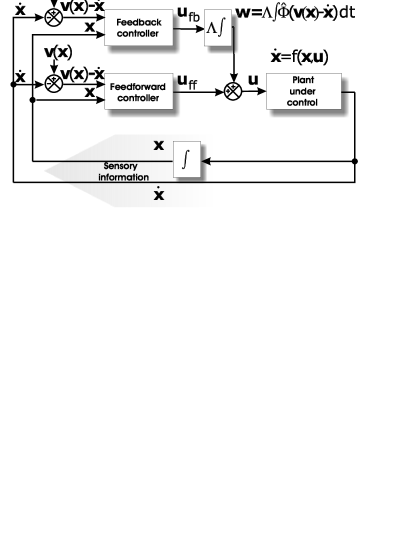
Figure 4. Robust speed-field tracking controller using differences between desired and experienced quantities
Feedforward and feedback controllers are the same, the output of the latter is integrated over time, amplified and is added to the output of the former to control the plant. Both controllers make use of the simplified inverse dynamics of Fig. 3(B) and both controller is inputted by the desired compensation $\mathbf{e}_{c}=\mathbf{v}(\mathbf{x})-\mathbf{\dot{x}}$. The scheme produces globally stable control under suitable conditions (Appendix 5.1).

Figure 4 can be further simplified (i) by assuming a first order plant, i.e., a plant with dynamical equation $\mathbf{\dot{x}}=\mathbf{f}(\mathbf{u})$ being independent of the actual state and (ii) by neglecting the feedforward controller. Now, the experienced variable is $\mathbf{x}$, whereas the desired variable is the desired state denoted by $\mathbf{\hat{x}}$. The corresponding architecture is shown in Fig. 5(A). Figure 5(B) depicts a loop made of neural network layers with the same dynamical properties (Appendix 5.3). From now on, let $\mathbf{W}$ and $\mathbf{Q}$ denote the ‘bottom-up’ (BU) and the top-down (TD )connections of the reconstruction network, respectively. There is, however, a subtle difference between the two architectures: The control network starts from a planned desired state $\mathbf{\hat{x}}$ and acts upon the plant to experience that state. The reconstruction network experiences the state (i.e., the input) $\mathbf{x}$ and acts upon a hidden layer to produce an the internal representation $\mathbf{h}$ of the network, which generates a reconstructed input $\mathbf{y}$ that should match the experienced input. The reconstruction network is an auto-associator, equipped with a hidden layer [45, 46]. The reconstruction network is also a comparator that minimizes the reconstruction error $\mathbf{e}=\mathbf{x}-\mathbf{\hat{x}}$. It is worth noting that the sign of the difference is the opposite as it is in the control architecture. The reason is that reconstruction network follows the environment, whereas control architecture manipulates it. The reconstruction network

1. generates the reconstructed input $\mathbf{\hat{x}}$ via the ‘top-down’ (TD) transformation, which is inputted by the hidden internal representation $\mathbf{h}$,

2. compares the input with the reconstructed input and produces the reconstruction error $\mathbf{e}=\mathbf{x}-\mathbf{\hat{x}}$,

3. processes the reconstruction error via the ‘bottom-up’ (BU) transformation and corrects the internal representation by that. (In continuous time, adding up ‘corrections’ is equivalent to the temporal integration of the error.)

Under certain conditions – matrix $\mathbf{WQ}$ of Fig. 5(B) should be positive definite (see Appendix 5.3) – error compensation converges and the network relaxes.

(12) $$\mathbf{\dot{h}}=\mathbf{W}(\mathbf{x}-\mathbf{Q}\mathbf{h})$$

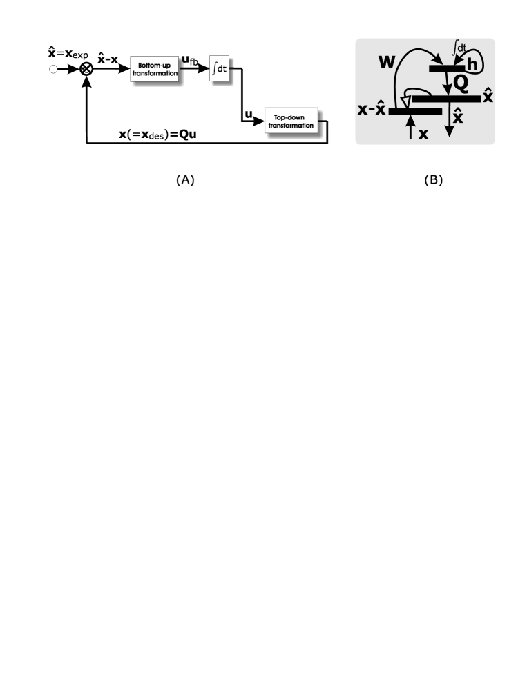
Figure 5. Control architecture for first order plant and the equivalent reconstruction network
A: Control architecture for first order plants and without feedforward controller.
For first order plant, the desired quantitiy is the desired state, whereas the experienced quantity is the experienced state. For the sake of comparison with subfigure B, desired state and experienced state are denoted by $\mathbf{x}$ and $\mathbf{\hat{x}}$, respectively.
B: The corresponding reconstruction network.
Reconstruction network with the same dynamical properties. Input (vector) $\mathbf{x}$ is provided to the network. Input is compared to ‘reconstructed input’ (vector) $\mathbf{\hat{x}}$, which is generated by internal representation (vector) $\mathbf{h}$ through the ‘top-down’ (TD) transformation (matrix) $\mathbf{Q}$. Mismatch (vector) $\mathbf{x}-\mathbf{\hat{x}}$ is delivered to correct the internal representation via ‘bottom-up’ (BU) transformation (matrix) $\mathbf{W}$. Correction is achieved by temporal integration (i.e., adding up the correcting term and applying recurrent self-excitations) at the level of the internal representation. Note the switch between experienced (sensed) and desired (to be matched) quantities.

2.3. Extended reconstruction network

The reconstruction network of Fig. 5(B) can be extended to fulfill particular constraints and computational tasks. The extended network is depicted in Fig. 6. The working of the network can be understood as follows:

Figure 6. Extended and controlled reconstruction network architecture
Arrow with circle denote non-linear transformation. $\mathbf{x}$ and $\mathbf{\hat{x}}$: input and reconstructed input, $\mathbf{W}$ and $\mathbf{Q}$: bottom-up (BU) and top-down (TD) transformation, $\mathbf{s}$: BU processed reconstruction error with maximized information, $\mathbf{h}$: activity vector of the hidden (model) layer, $\mathbf{N}$: transformation from BU processed reconstruction error layer to the model layer, $\mathbf{P}=\mathbf{QN}^{-1}$: BU matrix of the inner loop, $f(\mathbf{P}\mathbf{\hat{x}})$ BU gate releasing vector, with sparsifying non-linearity $f(.)$, $\mathbf{B}$ and $\mathbf{v}$: tools of control. The reconstruction network can be considered as the environment of the control network, which provides the control vector $\mathbf{B}\mathbf{v}$. $\mathbf{v}$ is the desired momentum. Black: Reconstruction network architecture. Black and gray together: controlled reconstruction network.

Sensory input vector $\mathbf{x}$ is compared to the reconstructed input vector $\mathbf{\hat{x}}$. The error $\mathbf{e}=\mathbf{x}-\mathbf{\hat{x}}$ is transformed by the bottom-up (BU) transformation matrix $\mathbf{W}$ and forms the BU transformed error $\mathbf{s}$. BU transformation maximizes BU information transfer in order to facilitate reconstruction. BU transformed error is passed to the internal representation layer through transformation matrix $\mathbf{N}$ (the role of this transformation shall be discussed later) and is added to the internal representation $\mathbf{h}$ of the ‘hidden’ (or model) layer. The activity of the hidden layer is maintained by diagonal elements of recurrent matrix $\mathbf{M}$. Considering the BU error correction, matrix $\mathbf{M}$ can serve temporal integration.

Beyond this temporal integration, off-diagonal elements of associative matrix $\mathbf{M}$ can perform temporal prediction [104, 16, 100].

Reconstruction vector $\mathbf{\hat{x}}$ is generated by TD matrix $\mathbf{Q}$. Note that any column of matrix $\mathbf{Q}$ could be equal to (different) individual inputs. In this case, reconstructed input will be the optimal linear combination of the individual inputs. However, the learning principles of this TD matrix can be more sophisticated than such a fast imprinting-like encoding.

Our specific assumption on TD matrix $\mathbf{Q}$ is constrained by our proposal on the resolution of the homunculus fallacy: the function of the hidden layer should be spatio-temporal pattern completion. Spatial pattern completion using prewired or experienced correlations can complete missing pieces of information. Representations using single (i.e., positive) sign empower the learning of correlations. Algorithms capable of finding positive components are called positive (non-negative) matrix factorization algorithms [99, 65, 145]. Positive matrix factorization together with pattern completion algorithms may imply [124] recognition by components [8]. That is, TD matrix $\mathbf{Q}$ is assumed to accomplish positive matrix factorization. Matrix $\mathbf{Q}$, which plays a major role in determining the relaxed hidden activity, is considered the long-term memory of the network.

As inner loop is introduced in Fig. 6 to perform non-linear noise filtering or sparsification of the BU processed error. The sparsification matrix $\mathbf{P}=(\mathbf{QN})^{-1}$ transforms reconstruction vector $\mathbf{\hat{x}}$. Components of the output of this transformation form the gate opening vector. If a component of this gate opening vector is below a certain threshold then the corresponding component of the BU processed error is diminished. There are theoretical works underpinning the idea: It has been shown that wavelet denoising [85] can be generalized to different databases using independent component analysis (ICA) [55, 18, 64, 7, 14, 2, 57, 1]. For a recent review on ICA, see [51]. ICA maximizes information transfer under the assumption that there are hidden factors and the probability distribution of these factors is equal to the product of the probability distribution of the individual components. Estimations based on ICA components are local: each component can be estimated separately.

Thresholding of independent components, alike to thresholding of wavelet components decreases the structureless noise content of the reconstructed input [52, 50]. The method is called sparse code shrinkage (SCS). Relation between SCS and an overcomplete reconstruction network with sparsifying non-linearity [95] has also been established [52, 50].

Theoretical considerations [76, 80] indicate that (i) matrices $\mathbf{P}$, $\mathbf{Q}$, $\mathbf{N}$, $\mathbf{W}$ can be tuned by Hebbian means. (ii) The reconstruction process diminishes some of the components of the input by projecting into to the subspace determined by the columns of matrix $\mathbf{Q}$. (iii) Matrix $\mathbf{P}$ performs ICA on the reconstructed input and thus denoising concerns the subspace of matrix $\mathbf{Q}$. (iii) Matrix $\mathbf{W}$ performs ICA on the input and the two ICA transformations may differ. (iv) Upon tuning, matrix $\mathbf{QNW}$ becomes the identity matrix and (v) matrix $\mathbf{P}$ becomes equal to matrix $\mathbf{W}$ and both perform the same ICA transformation. (vi) The speed of tuning for matrices $\mathbf{P}$, $\mathbf{Q}$ and $\mathbf{W}$ should be such that tuning of TD matrix $\mathbf{Q}$ is the slowest and tuning of BU matrix $\mathbf{W}$ is the fastest. We shall return to these points later. In turn, this network does the following: (i) learns to predict (near) future, (ii) maximizes BU information transfer, and (iii) filters noise.

2.4. Working of the extended architecture under control

2.4.1. Working of the extended architecture

The extended and controlled architecture satisfies the following non-linear equations:

(13) $$\mathbf{\dot{h}}=\underbrace{\mathbf{N}}_{(A)}f_{\mathbf{P}\mathbf{\hat{x}}}(\mathbf{W}\underbrace{(\mathbf{\hat{x}}-\mathbf{x})}_{(B)}+\underbrace{\mathbf{M}\mathbf{h}}_{(C)}+\underbrace{\mathbf{B}\mathbf{v}}_{(D)},$$

where BU error $\mathbf{e}=\mathbf{\hat{x}}-\mathbf{x}$ is the mismatch between input and reconstructed input. This error vector undergoes BU transformation (matrix $\mathbf{W}$) and forms the BU error vector. Components of the BU error vector (Eq. 13B) are subject to sparsification (function $f_{\mathbf{P}\mathbf{\hat{x}}}(.)$) where matrix $\mathbf{P}$ is determined by matrix $\mathbf{Q}$. Matrix $\mathbf{M}$ (Eq. 13C) is responsible for temporal integration, for prediction and for component based completion of spatio-temporal patterns [80].

2.4.2. Control of the extended architecture

The reconstruction network of Fig. 6 can be controlled by acting on the internal representation. This is the fourth term (D) of the r.h.s. of Eq. 13. Control adds extra contribution, i.e., $\mathbf{B}\mathbf{v}$ to the hidden layer. Vector $\mathbf{v}$ – which can be a function of the internal representation $\mathbf{h}$ ($\mathbf{v}=\mathbf{v}(\mathbf{h})$) – is the desired momentum. From the point of view of the controller, either $f(\mathbf{W}(\mathbf{\hat{x}}-\mathbf{x}))$ or its linear transform $\mathbf{N}f(\mathbf{W}(\mathbf{\hat{x}}-\mathbf{x}))$ can serve as the experienced momentum. Clearly, there is no warranty that the experienced momentum will match the desired one, unless matrix $\mathbf{B}$ is properly tuned. For a learning system, this match can not be warranted and thus a robust control scheme that can enforce the desired quantities becomes a necessity.

2.5. Reconstruction network controlled by a robust controller

The control scheme of Section 2.1 has several advantages (see Appendix 5.1):

1. As a result of the robustness, the learning of controlling is simplified: if the control action is sign proper, i.e., the control action takes the system into the good direction, then control is ultimately uniformly bounded and globally stable. Moreover, the bound of the tracking-error can be made arbitrarily small.

2. ‘Learning–by–doing’ can be accomplished during controlling, no matter if sign properness is fulfilled or not: the actual state and momentum are to be associated with the actual control vector.

Reconstruction network extended by the robust controller is depicted in Fig. 7(A) The working of the architecture on Fig. 7 can be understood as follows: First, let us consider the lower reconstruction network. This is the ‘plant’ (i.e., the ‘environment’) to be controlled. The controller is the upper reconstruction network. The lower network passes its experienced BU error ($\mathbf{\dot{x}}$) to the upper network through matrix $\mathbf{U}$. The effect of matrix $\mathbf{U}$ may be modulated by vector $\mathbf{V}\mathbf{h}$. The BU input to the upper network is $\mathbf{U}\mathbf{\dot{x}}$, which – up to a linear transformation – is equal to $\mathbf{\dot{h}}$. The desired momentum is provided by a particular transformation (not shown explicitly in any of the figures, but which is present in the neocortical structure [12, 13]) that originates from the internal representation and targets the corresponding reconstruction error layer of the same reconstruction network. We assume that this top-down signal is subtracted from the experienced momentum. The difference of the desired and experienced quantities forms the input to the feedforward controller. The output of the feedforward controller is $\mathbf{u}_{ff}=\mathbf{\hat{B}}(\mathbf{h})(\mathbf{v}(\mathbf{h})-\mathbf{\dot{h}})$. Note that matrix $\mathbf{\hat{B}}$ contains both BU and TD transformations. According to the working of the reconstruction network, the input, i.e., $\mathbf{v}(\mathbf{h})-\mathbf{\dot{h}}$, undergoes SCS noise filtering and temporal integration in the upper reconstruction network to make the reconstructed input. Apart from a linear transformation, this reconstructed input is the input to the feedback controller (Eqs. 5, 6 and Fig. 4). The output of the feedback controller is $\mathbf{u}_{fb}=\int\mathbf{\hat{A}}(\mathbf{h})(\mathbf{v}(\mathbf{h})-\mathbf{\dot{h}})dt$, where SCS noise filtering is not shown explicitly.

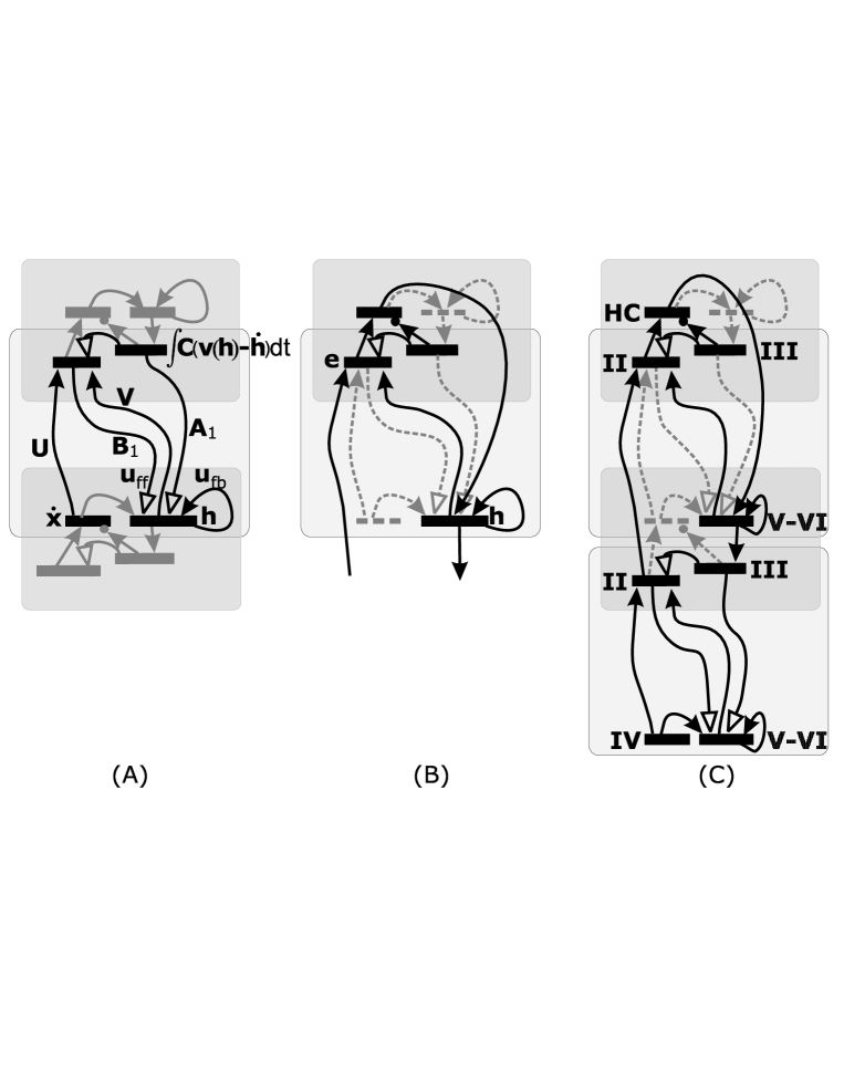
Figure 7. Robust control of the extended architecture
A: The two architectures, i.e., the reconstruction network and the robust control architecture are merged. Black color: components of the robust control architecture. Top and bottom: reconstruction networks. Matrix $\mathbf{U}$ carries $\mathbf{\dot{x}}$, the experienced speed. Also, $\mathbf{C}\mathbf{\dot{h}}=\mathbf{U}\mathbf{\dot{x}}$. Vector $\mathbf{V}\mathbf{h}$ may modulate the effect of matrix $\mathbf{U}$ and it can introduce state dependence. Matrices $\mathbf{A}_{1}$ and $\mathbf{B}_{1}$ are also components of the differencing controllers. $\mathbf{u}_{ff}=\mathbf{\hat{B}}(\mathbf{h})(\mathbf{v}(\mathbf{h})-\mathbf{\dot{h}})$. and $\mathbf{u}_{fb}=\int\mathbf{\hat{A}}(\mathbf{h})(\mathbf{v}(\mathbf{h})-\mathbf{\dot{h}})dt$ where matrices with hats comprise the effects of BU and TD transformations. (See text and Appendix 5.1.)
B: The top of the hierarchy. Dashed gray arrows and dashed gray levels do not belong to the architecture at the top. The top plays double role: (1)It is a reconstruction network. (2) It is a robust controller, because mismatch influences the activities of a hidden layer at a lower level.
C: The top of the hierarchy together with a lower robust controller. Roman letters represent corresponding sublayers of areas of the neocortical hierarchy. Dark gray areas: robust control, light gray boxes: neocortical layers, HC: hippocampus.

All components of the robust controller are now given and proper operation can be achieved, provided that transformations are sign-proper. In turn, the first and possibly the most problematic step of the learning task is the shattering of the state space to domains, within which the sign of control components does not change. Whereas the finding of the sign-proper domains may be a hard task, it is worth noting that there is no other condition imposed on the BU and TD matrices. For example, these transformations can be modulated vigorously, provided that sign-properness is kept (Appendix 5.1).

2.6. Working of the perfectly tuned hierarchy

Assume that all reconstruction networks are perfect: At all levels, the products $\mathbf{QNW}$ of Fig. 6 are equal to $\mathbf{I}$, the identity transformation. Assume that prediction is perfect, too. In this case, BU processing is error free, no error appears, no error correction occurs and, in turn, BU processing is as fast as in feedforward networks.

Similarly, for properly tuned inverse dynamics, top-down control will not produce error and top-down processing works also as a feedforward control architecture. These features are depicted for BU and TD processing in Fig. 8(A) and (B), respectively.

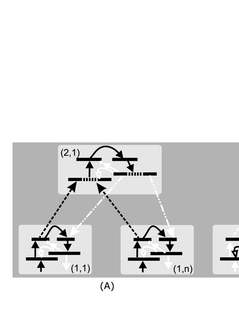
Figure 8. Bottom-up filtering (A) and top-down control (B) are both feedforward for perfectly tuned networks
Black arrows: the flow of information. White arrows: approximately silent connections.

2.7. Closing the loops of the hierarchy

We need to design the top of the sensory processing hierarchy. The top level receives information from different sensory systems, or modalities. Pattern completion may reveal that some of the components are missing or have been corrupted by noise and need to be fixed. To have a coherent interpretation, the top may need to correct such errors by influencing, i.e., controlling the internal representations of lower layers, the ‘environment’ of the top. In turn, we need a twist at the top: Mismatch between input and reconstructed input at the top should be also the mismatch between desired and experienced components. The two roles: reconstruction and robust control should be merged at the top. The solution is that the mismatch of the top reconstruction network is also the mismatch of the inverse dynamics effecting the hidden activity of a lower reconstruction network. This twist is shown in Fig. 7(B). Clearly, this is a reconstruction network with hidden layer $\mathbf{h}$ displaced. Figure 7(C) depicts the twisted top together with a lower control architecture. The hidden representation of the top reconstruction network has the double role form the point of view of its neighboring reconstruction error layers.

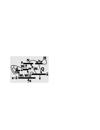
Figure 9. The top of the hierarchy and its mapping.
Maximization of BU information transfer is made in two steps: (i) whitening and (ii) ICA (separation). Blind source deconvolution sub-network has recurrent networks with long delays and removes temporal convolutions. Corresponding areas/layers in the loop formed by the hippocampus and the entorhinal cortex (EC): (i) reconstruction error (vector $\mathbf{e}=\mathbf{\hat{x}}-\mathbf{x}$): layer II of EC, (ii) reconstructed input (vector $\mathbf{x}$): layer III of EC, (iii) hidden or model layer (vector $\mathbf{h}$): layers V and VI of EC, (iv) recurrent loop of hidden layer (matrix $\mathbf{M}$): associative structure of EC layers V and VI, (v) BU processing layer in computational order (whitened reconstruction error $\mathbf{w}$ and separated reconstruction error $\mathbf{s}$): area CA3 and area CA1 of the hippocampus, respectively, (vi) BU matrices $\mathbf{W}_{1}$ and $\mathbf{W}_{2}$: EC afferents of the CA3 layer and Schaffer collaterals, respectively, (vii) recurrent loops with $\tau$ delays and vector $\mathbf{d}$: internal circuitry of the dentate gyrus and mossy cells of the dentate gyrus, respectively, (viii) matrix $\mathbf{W}_{3}$: perforant path afferents of the dentate gyrus, (ix) matrix $\mathbf{W}_{4}$: EC afferents of area CA1 of the hippocampus, (x) matrix $\mathbf{Q}$: deep layer to superficial layer connections of the EC, the long term memory components of the loop (xi) matrix $\mathbf{N}$: CA1 afferents of EC deep layers, the model layer of the loop.

This trick – that is the double role architecture at the top of the hierarchy – turns bottom-up processing to top-down control. However, there are additional constraints posed by information maximization: As long as lower networks are not properly tuned, processing is not feedforward and error correction gives rise to temporally convolved signals (Appendix 5.3). Temporal convolution corrupts the maximization of information transfer. In turn, temporal blind source deconvolution (BSD) [7, 137, 136, 66], is necessary.

As it has been emphasized by Lőrincz and Buzsáki [76], BSD in general, is very demanding. The number of neurons and the number of connections required by BSD are enormous. Fortunately, temporal convolution induced by reconstruction networks has special properties and, in principle, temporal deconvolution can be executed by a relatively small – but still ‘expensive’ – structure (see Appendix 5.3 for details). This structure needs recurrent connections with long and tunable delays. Given the robust control properties of the hierarchy, approximately correct signals can be enforced by starting from the top [75]. Thus, this expensive BSD structure is necessary only at the top of the hierarchy. BSD at the top deconvolves the reconstruction error before it is turned into a control signal. The reconstruction network together with BSD structure made of tunable delay lines is depicted in Fig. 9.

There is another difference between Figs. 6 and 9: BU processing is executed in Fig. 9 in two layers. The two layers perform two-step learning to maximize information transfer. The transformation to the first layer whitens (i.e., it decorrelates and normalizes components of the reconstruction error [64]), whereas the transformation to the second layer removes higher order correlations and, in turn, it develops independent components. The two step learning algorithm is fast, because it proceeds along the so called natural gradient (see, e.g., [1] and references therein). ICA can be slower in the BU sparsification transformation if it follows the one step learning rule of Bell and Sejnowski [7].

(14) $$\Delta\mathbf{P}\propto f(\mathbf{s})\mathbf{\hat{x}}^{T}+\mathbf{P}^{-1}$$

where $f(.)$ denotes component-wise non-linearity. This learning rule has two terms. One of them is a Hebbian term of the inputs and the outputs of matrix $\mathbf{P}$. The other term is proportional to matrix

(15) $$\mathbf{P}^{-1}=\mathbf{NQ}$$

that is to the rest of the loop. Matrix inversion, however, is not necessary, the second term can be approximated, e.g., by noise generated at the BU error layer and targeting the reconstructed input layer. The reconstruction architecture warrants this property through Eq. 15 [76, 80]. In turn, the order of learning is as follows: Novel structure not encoded into the TD matrix but embedded in mismatch vector $\mathbf{e}$ is blocked by SCS thresholding but undergoes fast ICA analysis and develops high amplitude BU error components, which can not be fully eliminated by thresholding. The access BU error undergoes temporal integration at the level of the internal representation. High activity components of vector $\mathbf{h}$ and high activity components of mismatch vector $\mathbf{e}$ will induce Hebbian learning in matrix $\mathbf{Q}$. This learning process is slow and it is followed adiabatically (i.e., very closely) by matrix $\mathbf{P}$. Given that learning of matrix $\mathbf{P}$ is subject to Hebbian learning between outputs of matrix $\mathbf{W}$ and reconstruction error produced by matrix $\mathbf{Q}$, learning of matrix $\mathbf{P}$ is kind of ‘supervised’ by these matrices: Upon TD matrix has incorporated the novel information, matrices $\mathbf{W}$ and $\mathbf{P}$ become equal, provided that no novel information has entered the loop. That is, we have the following scenario: (a) novelty is blocked, (b) matrix $\mathbf{W}$ is modified, (c) novelty is represented by a few large ICA components (i.e., a few components of BU error increases, whereas many components of BU error decreases), (d) large components overcome sparsification, (e) TD long-term memory changes slowly, (f) this slow change is closely followed by BU sparsification.

We note that a possible role of matrix $\mathbf{N}$ can be the whitening of the output of the BU error layer that underwent non-linear sparsification. This process, which advances Hebbian learning for matrix $\mathbf{M}$, will be discussed elsewhere [131].

3. Results: Straightforward mapping to sensory processing areas

Mapping – based on the reconstruction network description – has been thoroughly described elsewhere [76, 16, 80]. The control view [75] complements the basic structure of that mapping: beyond the function of connections between neocortical layers, it explains the function of connections of the neocortical layers that have not been modelled previously [80].

3.1. Mapping to neocortical regions

The neocortex is made of six sub-layers (Fig. 10(A)). The figure depicts the most prominent connections between these sub-layers [83]. Input typically arrives at layer IV. Layer IV neurons send messages to layer II and layer III (not shown). Furthermore, layer IV neurons send messages also to layer VI. Superficial neurons provide output down to layer V and VI. There are connections between neurons of layer V and layer VI. Neurons of layer II and III are also strongly connected. Layer V provide feedback to layers II and III. The main output to higher cortical layers emerges from layers II and III. The main feedback to lower layers is provided by layer V. (For a review see, e.g., [12].)

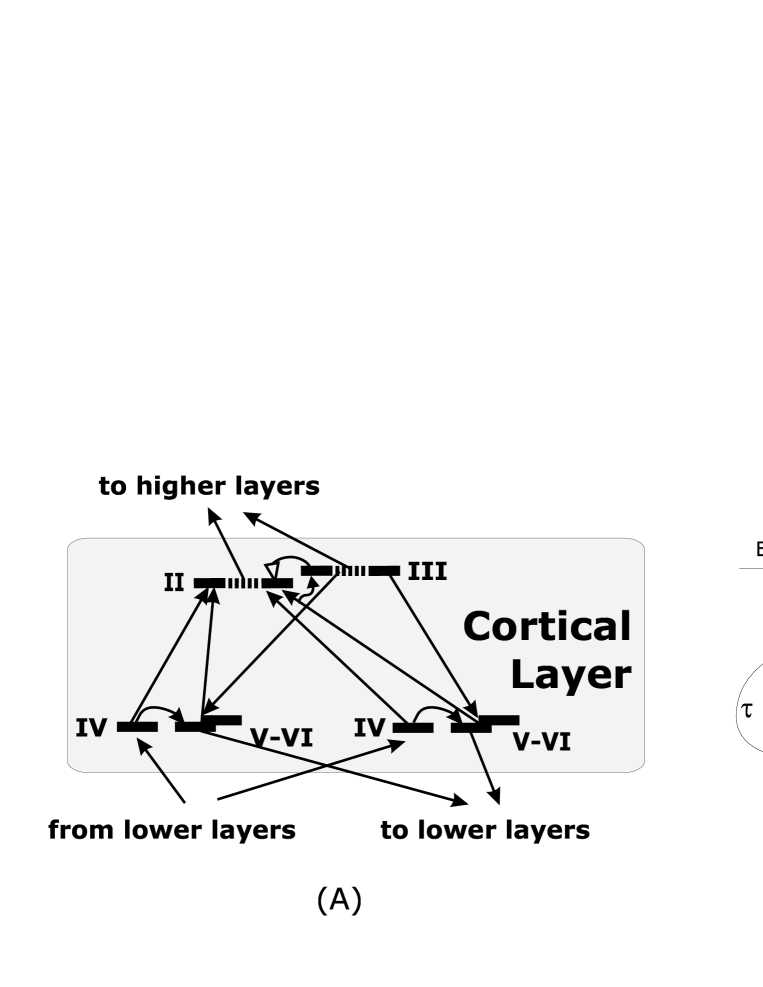
Figure 10. Neocortical circuitry and the dentate gyrus
A: Input: layer IV. Layer IV neurons send messages to layer II, layer III and layer VI. Layer V and layer VI neurons receive messages from layer II and layer III. Layer V neurons provide feedback to layers II and III. Neurons of layers V and VI are connected (indirectly shown by the proximity of these layers). Neurons of layer II and III are also connected (only inhibitory connections are shown). Feedforward output to higher cortical layers: layers II and III. Feedback to lower layers: layer V.
B: The excitatory connections between granule cells (g) and hilar mossy cells (mc) as well as in the g-CA3 pyramidal cells (p)-mc-g loop provide delay lines. Feedback inhibitory neurons innervate specific dendritic segments of the granule cells at the termination zone of the EC and mc afferents. HIPP: hilar interneuron with axonal termination in the perforant path zone; HICAP: hilar interneuron with axon termination in the commissural and association paths, mf: mossy fibers, $\tau$: synaptic delay. The activity of these interneurons also controls plastic changes (i. e., training) of the mc-gc synapses.

The theoretical model and the anatomical structure can be matched only by assuming that reconstruction networks are laid between neocortical layers as it was denoted by the dark gray areas in Fig. 7(A). On the other hand, robust control is executed by the cortical layers, the light gray boxes of Fig. 7(A). According to this figure, superficial layers of the lower cortical layer and deep layers of the higher cortical layer form one functional unit, the reconstruction network. The reconstruction error and the reconstructed input of this functional unit exert control action on lower reconstruction networks. This controller is inputted by the experienced state and by the BU processed reconstruction error (i.e., the experienced momentum) of the lower reconstruction network.

In this view, the V1 performs two functions: layers V and VI of the primary visual cortex hold the internal representation of the LGN, while layers II and III represent the input and the reconstructed input of V2, respectively.

3.2. Mapping to the hippocampal-entorhinal loop

The hippocampus (HC) is placed on the top of the hierarchy (Fig. 7(C)). The HC incorporates a unique subunit, the dentate gyrus, which, in our view, removes temporal convolution of lower reconstruction networks. Loops required for temporal deconvolution do exist in the dentate gyrus (Fig. 10(B)). Notably, extreme long delays (on the order of 500 ms), which is a crucial prediction of our model [76] has been found experimentally [44].

Besides temporal deconvolution, HC is also engaged in information maximization and performs whitening and separation (Fig. 9) performed by the CA3 and CA1 subfields of the hippocampus . According to our model, the hippocampus plays two roles:

1. HC acts upon the deep layers of the EC. In turn it can exert control action on the model layer of the EC.

2. HC and EC together, form a reconstruction network, the EC-HC loop. This loop is special in that it may perform blind source deconvolution on its inputs.

The two-phase operation of the loop [11] ensures correct order of learning: analyzing and maximizing BU information transfer and the encoding of top-down memory. Details about the mapping to the EC-HC loop as well as details about two-phase encoding can be found elsewhere [76]. According to that model, encoding of long term memory is initiated by the recurrent collaterals (not shown in the figure) of the CA3 area in one of the two-phases, the sharp-wave phase.

4. Discussion

4.1. Relation to other models

From the computational point of view, we should mention the model of Gluck and Myers [29], which was designed to perform reconstruction and classification together for modeling some properties of the hippocampus. This reconstruction idea gains also importance in a recent model of Stainvas et al. [122], in which reconstruction is used as regularization constraint in classification task for creating better representations.

Another approach has been proposed by Rao and Ballard. They have put forth an integrating model [104, 103, 105] by exploring a Kalman-filter analogy to cope with the input and system uncertainties (treated as noise) and presented a hierarchy for error correction and prediction using top-down inference from higher levels. For spatial learning tasks, another Kalman-filter based model has been proposed with a biological mapping to the hippocampus [9]. Kalman-filter is a kind of reconstruction or generative network, which uses an internal representation to generate expected inputs. Although the Kalman-filter idea could be an efficient and plausible function for sensory processing, the mapping of the proposed function onto the anatomical, neurophysiological findings has not been elaborated. Another problem is that noise filtering in Kalman-filters requires matrix inversions. Also Kalman-filters form loops, which are generally slow for the processing speeds found in neocortical areas. Apparently, sensory processing in neocortical areas is feedforward [63].

4.2. Algorithmic components of the CHF model

The CHF has two basic components: (1) the reconstruction network and (2) a robust control architecture.

1. According to Horn [48], vision is inverse graphics. Our model generalizes this view by the old standing proposal that the hippocampus and its environment serve as a ‘comparator’ [32, 120, 139]. Auto-associators with hidden layers [46], i.e., reconstruction networks come to the sight by considering these two suggestions together.

2. The control aspect of sensory processing has been suggested long time ago: According to Diamond [22] layer V could be seen as an extension of the motor cortex in all areas, because layer V neurons send inputs to basal ganglia, brain stem and sometimes even to the spinal cord. This conjecture is reinforced by our mapping, where layers V exert control actions on lower neocortical areas.

The CHF model makes use of maximization of information transfer in sensory processing, first suggested by Attneave [5] and Barlow [6]. We note that ICA produces optimal representation for mean-field approximation that empowers local (i.e., fast) approximation for inferencing (information extraction from uncertain observations) [39].

One of the main algorithmic components of the CHF model, the so called sparse code shrinkage (SCS) performs database optimized denoising [52, 50]. The intriguing point is that denoising is experience based and, in turn, novelty – at first sight – may appear as noise. The high ‘noise content’ blocked by sparsification is a direct sign of the possibility of novel information. Novelty detection that precedes recognition (the searching of the database) has been an old mystery of information processing in the brain. The SCS algorithm placed into the reconstruction network offers a solution here (see later).

Speed-field tracking (SFT) based controlling is the other main component of our model. Efforts have been made to derive the entorhinal-hippocampal loop [75] starting from SFT. It can be motivated by

1. the opinion that the medial paralimbic system (that includes the supplementary motor area as well as the anterior cingulate cortex, and that develops the elaborated basal ganglia thalamocortical loops) originates from the hippocampal cortex [111, 30] and the strength of speed-field tracking in modelling those basal-ganglia thalamocortical loops [72, 77],

2. the control aspect of layer V of neocortical areas [22],

3. the view that the brain formulates signals that specify positions and directions of targets in extrapersonal space (see, e.g., [146]) that resembles speed-field with dynamic path planning capacity [26, 130],

4. the mathematical tractability of speed-field tracking based control architecture [126, 129, 128].

4.3. Arguments for the CHF model

4.3.1. Experimental evidences

As it has been noted in the introduction, two predictions of the model, (a) large and tunable temporal delaying capabilities of neurons of the dentate gyrus and (b) persistent activities at deep layers of the EC have been reinforced recently in [44] and in [23], respectively. This latter prediction follows from the temporal integration at the model layer, which are at the deep layers of the EC. In turn, the CHF model has already passed two falsifying predictions.

4.3.2. Implicit memory effects, order of learning

Order of learning:

Learning steps warranted by the model are as follows:

1. The possibility of novelty is signaled by non-sparse BU processed error activity pattern.

2. BU processed non-sparse activities, such as noise or novel information are gated by sparsification.

3. ‘Noise’ constantly undergoes fast maximization of information transfer in the BU processed error channel via ICA. Denoising (sparsification) cannot withhold high amplitude components of the BU processed error and information (i.e., structure embedded in noise) become available to the hidden layer of the model.

4. Structured information is encoded into the top-down matrix, the long-term memory of our model.

In turn, the architecture learns structure and rejects noise.

Some implicit memory effects emerge directly from the CHF model.

Repetition priming:

The term ‘priming’ in a broader sense refers to the observation that an earlier encounter with a given stimulus can modify (‘primes’) the responding to the same or a related stimulus (see, e.g., [107] and references therein).

It has been shown by numerical simulations of reconstruction networks using ICA for BU information maximization that repeated presentations of not yet learned (novel or partially novel) inputs shortens relaxation time of the reconstruction architecture without modifying LTM. The experienced decrease of relaxation time has been interpreted as priming [82]. It can also be demonstrated that this effect is enhanced by SCS denoising .

Repetition suppression and repetition enhancement:

The neuronal correlate of priming is thought to be repetition suppression [21]. This belief is supported by the joint appearance of the two phenomena in many experiments, see, e.g., [10, 87]: Both cognitive and neurophysiological experiments show that neurons in the neocortex respond with less and less activity in the case of repeated stimuli (see e.g., [113] and references therein). This repetition decrement is often called ‘repetition suppression’ in the primate literature [142]. Numerical experiments demonstrate that repetition suppression appears jointly with the shortening of relaxation time [82] in extended reconstruction networks. An intriguing phenomenon is that during repetition suppression, a few neurons do exhibit repetition enhancement [21]; an emergent property of our model: Repetition enhancement is shown by those few units, which upon information maximization become strongly activated and can break through the threshold of sparsification [82].

Distributed nature of implicit memory effects:

It is known that implicit memory effects, such as the recognition of novelty, is distributed [140]. The order of learning – as described at the beginning of this subsection – warrants that these effects, including novelty detection, may occur at every reconstruction network and, in turn, it is distributed in the CHF model. Similarly, the comparator function is distributed in the model, too.

Prototype learning:

Recent research has provided evidence that category learning is mediated by multiple neuronal systems in the brain (see, e.g., [3] and references therein, but see [92]). In contrast, when information is accumulated from many exemplars and no verbal rules are easily available, implicit mechanisms related to the basal ganglia may operate. A good example for this latter type is a classic prototype learning paradigm [101, 62, 61]. Interestingly, prototype learning, which is spared in patients with HC damage [62] is impaired in Alzheimer patients [59, 58]. In reconstruction networks, many exemplar based prototype learning may emerge in different ways. We have also demonstrated that the adaptation of the recurrent excitatory connections of the hidden layer [4, 60] can explain the impairment found in Alzheimer patients. Another candidate structure is the recurrent excitatory connections of superficial layers. These recurrent connections have not been included into the CHF model yet. Their function will be conjectured later.

4.3.3. Temporal compression

The recurrent excitatory connections of the deep layers, which perform spatio-temporal pattern completion, and the error-correcting associative connections of the superficial layers, together, fulfill the requirements of temporal compression if network operation is not continuous but periodic [138]. Such temporal compression has been observed in the hippocampus [94, 119].

4.3.4. Specific properties vs. generalization

McClelland et al. [86] emphasize the necessity of a dual system for the seemingly contradictory tasks of learning of specific properties and allowing for generalization. The CHF model allows for an attractive solution here: Specific properties can be encoded into the LTM, whereas generalization is allowed by the flexible combination of LTM components at different levels of the hierarchy by the control means. TD control, up to the limits imposed by sign-properness, can distort, combine, and excite memory components.

4.3.5. Mathematical issues

Adaptation and learning rules:

As it has been described elsewhere [76, 80], the loop structure is advantageous for Hebbian learning. Neural activities and noise, together, with a relatively long (5̃0 ms) temporal window are required for whitening and the learning of independent components in both BU pathways. Top-down matrices are trained by the reconstruction error and the hidden layer activity (the delta rule); the necessary signals for Hebbian learning are available between the model layer and the reconstruction error layer [76, 80].

The controller can learn by experimenting, i.e., by the learning-by-doing scheme [26]. No matter what the desired parameters are, the experienced parameters need to be associated to the control parameters to form an approximate inverse dynamics. When the approximation becomes sign-proper, the control architecture will be approximately precise [77].

Adaptation of the robust controller is straightforward and occurs via error feedback and temporal integration. It is an attractive property of the control architecture that fast temporal changes of different transformations of different networks of the hierarchy (i.e., learning) can not disturb the stability of the controller as long as the control remains sign-proper (Appendix 5.1)

Noise in the controller:

It has been noted in [126] that the SDS scheme is sensitive to noise if the noise enters the system just before the compensatory vector is integrated, i.e., if noise affects $\dot{{\bf w}}=\mathbf{u}_{fb}$ of Eq. 8. Such a noise can easily make the system unstable, because the perturbation takes the form

$$\Lambda\int_{0}^{T}n(t)dt,$$

where $n(t)$ denotes the noise. Unfortunately, the boundedness of integral of Eq. 8 cannot be ensured for the general case. Moreover, the amplitude of the perturbation will be proportional to $\Lambda$. This means that increasing $\Lambda$ will also increase the perturbation of the system. This problem is the problem of every dynamic state feedback controller provided that noise can enter precisely before the point where the compensatory control signal is integrated through time. It is an emerging feature of the CHF architecture that this problematic noise component can be diminished by optimized SCS denoising.

On the other hand, the presence of noise is necessary and advantageous in the CHF model. It is necessary for Hebbian learning [76] and it is also advantageous to improve generalizing capability of ICA [53].

Reinforcement learning and behavioral relevance:

It is a central issue if the robust controller can be incorporated into the reinforcement learning (RL) framework or not. This problem has been treated theoretically and answered positively: The integration of robust controller and RL is possible within the so called event learning framework, a novel form of reinforcement learning [78, 134, 135, 79]. In this scheme, time is broken into discrete time intervals and, if temporal resolution is sufficient then, near optimal performance with uncertain state descriptions can be achieved. Some parameters that might change considerably (e.g., the mass [128] or the length of a robotic arm [77]) may be left unobserved without affecting near optimality, a rare feature in RL models. Furthermore, the robust controller fits smoothly the reinforcement learning interpretation of dopamine responses found in the basal ganglia [115, 74]. Considering behavioral relevance, there is no decision-making system embedded into the CHF model; the CHF model is passive. On the other hand, we have succeeded to show that the CHF model, including the reconstruction loop architecture and the robust controller can be embedded into the reinforcement learning framework and near optimal performance will be warranted. In turn, the model can be easily extended by decision-making and planning.

In the CHF network, the hidden variables are controlled. It is then another issue if a model with hidden variables can be optimized using RL. We note that Kalman-filters, which are tractable from the point of view of mathematical considerations, can be seen as the mathematical approximation of the CHF scheme. Kalman-filters have been integrated into the reinforcement learning framework and convergence to the optimal solution is warranted [132, 133]. To our best knowledge, this is the first case when a partially observed Markovian decision problem is shown to converge and to learn the optimal policy. One emerging property of the derivation is that the learning rule for the value of states has a Hebbian form [132]. The weight factor of the learning rule is proportional to the error of value prediction. Based on this observation we may remark the followings:

Note (1) The CHF model, alike to its previous versions [75, 76, 80] is neither a model for episodic learning, nor a model for incremental learning and does not fit such traditional distinctions (see, e.g., [28]). On the one hand, when information maximization is not modulated by behavioral relevance, the CHF model is an incremental model. On the other hand, the CHF model can be instantaneous, if behavioral relevance (i.e., error in value estimation) increases learning efficiency. Error in value estimation can modulate the Hebbian learning rule of LTM and, in turn, input can be immediately encoded into the reconstruction architecture.

Note (2) Long-term memory of the CHF model are not permanent; they may change. Changes are subject to statistical properties of the information (because information transfer is to be maximized) and to behavioral relevance of the information. That is, in the CHF model, ‘memory traces are unbound’ [91].

4.4. Conjectures

The CHF model allows us to make predictions. Some of the conjectures qualify as attractive possibilities offered by the CHF model, whereas others are falsifying predictions.

Principles of learning bottom-up and top-down transformations may apply for the learning of the predictive matrix (i.e., matrix $\mathbf{N}$) of the hidden layer, too. It is easy to show that minimization of the square of the prediction error may lead to Hebbian learning for this matrix and has the following form:

(16) $$\Delta\mathbf{M}\propto\left(\mathbf{N\dot{h}}\right)\mathbf{h}^{T}$$

provided that three conditions are met: (i) connections (synapses) have access to the corresponding hidden layer activities, i.e., to $\mathbf{h}$. (ii) The same connections have access to the error of the hidden layer activities on the other side, i.e., to $\mathbf{N\dot{h}}$ and (iii) input to the hidden layer is whitened to avoid the necessity of multiplication by the inverse of the correlation matrix $C(\mathbf{h},\mathbf{\dot{h}})$. From condition (iii) it is conjectured that transformation $\mathbf{N}$, which corrects the activity of the hidden layer, whitens the sparsified BU error. This transformation has remained unconstrained: The prescribed identity transformation of the full loop can be achieved by rescaling matrices, e.g., the top-down matrix. Whitening is also advantageous from the point of view of learning: The learning rule of Eq. 16 follows the natural gradient [2]. Condition (ii) implies that one of the deep layers holds this whitened BU error, whereas the other holds the hidden activities. Local circuits between the two layers can provide the appropriate Hebbian training signals. Given that neurons of layer V play control roles, it is layer VI, which can hold the whitened BU error. If this is the case, indeed, then sustained activity of neurons of layer V may be more pronounced than that of neurons of layer VI.

The role of associative structures in the superficial layers is not apparent in the CHF model. It is conjectured here that these associative connections may serve error correction. We need to tell error correction and pattern completion apart. Here, pattern completion concern spatio-temporal patterns. Error correction, on the other hand, is seen as a synchronous operation over actual inputs, alike in content addressed memories [38] or Hopfield network-like constructs [143]. The dynamic Hopfield model [56] is a candidate CNS model for layers with recurrent collaterals. Note that in the CHF model [76] the recurrent collateral system of the CA3 subfield elicits randomly ordered temporal replays of input sequences and serves to encode information into the top-down memory and to diminish weak connections to improve generalization capabilities [53]. This replaying role is supported by experimental evidences [144, 118, 90, 47].

Feedback connections between neocortical layers are generally more numerous than the feedforward connections between neocortical layers and these connections seem to have a weak functional role (see, e.g., [12] and references therein). Also, interaction within neocortical layers is much stronger than feedback activities. On the other hand, these feedback connections play a central role in the CHF model; these connections form the long term memory of the architecture. In our view, this is an apparent contradiction. The trick is that reconstruction is fast and easy and, in the CHF model, it is feedforward in a well tuned network. The hard problems are (i) how to choose amongst the different possibilities, i.e., the ‘negotiation’ between different neocortical columns, different neocortical areas and different sensory modalities. The possibility that different interpretations may coexist in the brain has been made evident in the animal experiments on binocular rivalry (see, e.g., [68] and references therein) and in experiments with several possible visual interpretations [67]. (ii) How to express the decisions that have been made? It is expected that on-going control signals – no matter if conscious or not – are separated from background noise by synchronous operation. Such synchronous signals dominate the reconstruction process.

Falsifying prediction 1. An intriguing conjecture of the CHF model is that disturbance of the feedback connections between neocortical layers may corrupt apparent feedforward processing and recognition but should not corrupt prototype learning.

Falsifying prediction 2. The CHF model allows us to claim that perceptual learning (see, e.g., [114] and references therein) and categorical perception (see, e.g., [31, 40] and references therein) are two manifestations of the same long-term memory effects. If so then (i) the place of encoding should include almost exclusively the top-down LTM components of areas engaged in sensory processing and (ii) frequent appearance without strong behavioral relevance will barely modify the same components. Nevertheless, modified inputs to higher layers may influence bottom-up processing in areas above the place of encoding.

5. Appendices

5.1. Appendix A: Robustness and stable on-line adaptation

A plant is called first order if its ‘position’ (or configuration) determines the state of the plant and if the dynamical equation determines the momentum (of all parts of the plant). A plant is called second order if the state is given by the configuration and the momentum and if the dynamical equation determines the acceleration, and so on. Higher order plants can be rewritten into the form of a set of first order differential equations by concatenating ‘position’, ‘momentum’, etc. into the state vector (see also Appendix 5.2).

Speed field tracking (SFT) is not typical in the control literature, but arises naturally if we consider stationary optimal-control problems such as path planning tasks [49]. Conventional control tasks, such as point-to-point control and trajectory tracking cannot be exactly rewritten in the form of SFT and vice versa [126, 127]. SFT prescribes the speed vector $\mathbf{\dot{x}}$ of the plant as a function of the state vector:

(17) $$\mathbf{\dot{x}}=\mathbf{v}(\mathbf{x})$$

SFT task has the advantage that the designer can incorporate several objectives into the form of the speed-field to be tracked hence extend the model’s range of possibilities.

The mathematical treatment described here is a slight generalization of that of published in [128, 126]. The control scheme works for plants of any order, alike to the original proof. The identity of the feedforward and the feedback controllers is released. This slight generalization seems necessary to properly describe the superficial–to–deep layer wiring of the neocortex.

Let $D\subseteq\mathbf{R}^{n}$ denote the domain of the plant’s state with the equation of motion given by

(18) $$\mathbf{u}=\mathbf{B}(\mathbf{x})\mathbf{\dot{x}}+\mathbf{b}(\mathbf{x})$$

where $\mathbf{x}$ is the state vector of the plant and $\mathbf{u}\in\mathbf{R}^{m}$ is the control. For simplicity the dependence of $\mathbf{B}$ and $\mathbf{b}$ on $\mathbf{x}$ will not be explicitly represented. Now let us assume that we have two estimates of the true inverse-dynamics function $\Phi(\mathbf{x},\mathbf{\dot{x}})=\mathbf{B}\mathbf{\dot{x}}+\mathbf{b}$, given by $\mathbf{\hat{\Phi}}(\mathbf{x},\mathbf{\dot{x}})$ and $\mathbf{\hat{\Psi}}(\mathbf{x},\mathbf{\dot{x}})$:

(19) $$\mathbf{\hat{\Phi}}(\mathbf{x},\mathbf{\dot{x}})=\mathbf{\hat{B}}\mathbf{\dot{x}}+\mathbf{\hat{b}}$$

(20) $$\mathbf{\hat{\Psi}}(\mathbf{x},\mathbf{\dot{x}})=\mathbf{\hat{A}}\mathbf{\dot{x}}+\mathbf{\hat{a}}$$

The SDS Feedback Control equations can then be written as

(21) $$\mathbf{u} = \mathbf{u}_{ff}(\mathbf{x},\mathbf{\dot{x}},\mathbf{v}(\mathbf{x}))+\mathbf{w},$$

(22) $$\mathbf{\dot{w}} = \Lambda\left(\hat{\Phi}(\mathbf{x},\mathbf{v}(\mathbf{x}))-\hat{\Phi}(\mathbf{x},\mathbf{\dot{x}})\right)$$

where $\mathbf{u}_{ff}$ is the so called feedforward controller (to be specified later), $\Lambda>0$ is the gain of feedback.

In what follows the usual definition of positivity for fields of square matrices will be required.

Definition. Let $\mathbf{M}:D\rightarrow\mathbf{R}^{p\times p}$, $p>0$. $\mathbf{M}$ is said to be positive definite uniformly over $D$ iff for all $\mathbf{x}\in D$ the term $\mathbf{M}(\mathbf{x})$ is positive definite and there exists an $\epsilon>0$ such that $\lambda_{\min}(\mathbf{M(}\mathbf{x}))>\epsilon$ holds for all $\mathbf{x}\in D$. Uniform negative definiteness can be similarly defined.

If $\mathbf{M}$ is a real quadratic matrix then let $\mathbf{M}>0$ denote that $\mathbf{M}$ is positive definite. Similarly, if $\mathbf{M}$ is a matrix field over $D$, let $\mathbf{M}>0$ denote that $\mathbf{M}$ is uniformly positive definite over $D$ .

Theorem. Assume that the feedforward controller has the form

$$\mathbf{u}_{ff}(\mathbf{x},\mathbf{\dot{x}},\mathbf{v})=\mathbf{\hat{\Psi}}(\mathbf{x},\mathbf{v})-\mathbf{\hat{\Psi}}(\mathbf{x},\mathbf{\dot{x}}),$$

which is similar as the input of the feedback integrator. Further, assume that the followings hold:

1. $\mathbf{\hat{\Phi}}(\mathbf{x},\mathbf{\dot{x}})=\mathbf{\hat{B}}\mathbf{\dot{x}}+\mathbf{\hat{b}}$

2. $\mathbf{\hat{\Psi}}(\mathbf{x},\mathbf{\dot{x}})=\mathbf{\hat{A}}\mathbf{\dot{x}}+\mathbf{\hat{a}}$

3. $\mathbf{X}^{T}\mathbf{Y}$, where $\mathbf{X}$ and $\mathbf{Y}\in\{\mathbf{A},\mathbf{\hat{A}},\mathbf{\hat{B}}\}$ are uniformly positive definite over $D$

4. $\mathbf{A}$, $\mathbf{v}$, $\mathbf{b}$ are bounded and have uniformly bounded derivatives w.r.t. $\mathbf{x}$ over $D$

Then for all $\Lambda>0$ the error of tracking $\mathbf{v}(\mathbf{x})$, $\mathbf{e}=\mathbf{v}(\mathbf{x})-\mathbf{\dot{x}}$, is eventually uniformly bounded and, further, the eventual bound $b$ of the tracking-error can be made arbitrarily small. More specifically $b=\mathcal{O}(1/\Lambda)$, and the eventual bound for the time reaching $||\mathbf{e}||\leq b$ is proportional to $\Lambda$.

The proof of this theorem relies on a Liapunov-function approach. First of all, note that $\mathbf{\dot{w}}=\Lambda\mathbf{\hat{B}}(\mathbf{v}-\mathbf{\dot{x}})$ and that $\mathbf{u}=\mathbf{\hat{A}}(\mathbf{v}-\mathbf{\dot{x}})+\mathbf{w}$. The relation $(\mathbf{B}+\mathbf{\hat{B}})\mathbf{e}=\mathbf{A}\mathbf{v}+\mathbf{b}-\mathbf{w}$ can be employed to show that $L={1\over 2}\mathbf{e}^{T}\left[(\mathbf{A}+\mathbf{\hat{A}})^{T}(\mathbf{A}+\mathbf{\hat{A}})\right]\mathbf{e}$ is an appropriate semi-Liapunov function. The proof starts by differentiating $\mathbf{e}$ according to time:

(23) $$\frac{d}{dt}\mathbf{A}\mathbf{v}+\mathbf{b}-\mathbf{w} = \frac{\partial(\mathbf{A}\mathbf{v}+\mathbf{b})}{\partial\mathbf{x}}\mathbf{\dot{x}}-\mathbf{\dot{w}}$$

(24) $$= \frac{\partial(\mathbf{A}\mathbf{v}+\mathbf{b})}{\partial\mathbf{x}}\mathbf{\dot{x}}-\Lambda\mathbf{\hat{B}}(\mathbf{v}-\mathbf{\dot{x}})$$

(25) $$= \mathbf{f}-\Lambda\mathbf{\hat{B}}\mathbf{e}$$

where $\frac{\partial\mathbf{x}}{\partial\mathbf{x}}$ denotes the Jacobi derivative matrix of vector $\mathbf{x}$ according to vector $\mathbf{x}$ and $\mathbf{f}=\frac{\partial(\mathbf{A}\mathbf{v}+\mathbf{b})}{\partial\mathbf{x}}\mathbf{\dot{x}}$. In turn, the temporal derivative of our semi-Liapunov function assumes the following form:

(26) $$\frac{d}{dt}L=\mathbf{e}^{T}(\mathbf{A}+\mathbf{\hat{A}})^{T}\left[\mathbf{f}-\Lambda\mathbf{\hat{B}}\mathbf{e}\right]$$

Then the proof can be completed by using the methods thoroughly detailed in [126]. The proof compares the two terms of the r.h.s. of Eq 26 and notes that the negative term, which can be made arbitrarily large, ensures uniform boundedness.

The subtle point of this theorem is the requirement that $\mathbf{A}^{T}\mathbf{\hat{A}}$ and $\mathbf{A}^{T}\mathbf{\hat{B}}$ should be uniformly positive definite over $D$. The theorem gives rise to a global stability result. Notice too that the particular form of the feedforward and feedback controllers make it unnecessary to build an estimate of $\mathbf{b}$.

Note that in the case of Eq. 26 there is no dependence on the approximated inverse-dynamics. This fact can be exploited to show that the above proof remains valid if $\mathbf{\hat{A}}$, $\mathbf{\hat{B}}$, $\mathbf{\hat{a}}$ and $\mathbf{\hat{b}}$ vary in time but the conditions of the theorem remain valid at every instant. Thus we get the following important corollary:

Corollary. Suppose that the conditions of Theorem hold and also that $\mathbf{\hat{A}}=\mathbf{\hat{A}}(t)$, $\mathbf{\hat{B}}=\mathbf{\hat{B}}(t)$, $\mathbf{\hat{a}}=\mathbf{\hat{a}}(t)$ and $\mathbf{\hat{b}}=\mathbf{\hat{b}}(t)$. Next assume that $\mathbf{B}^{T}\mathbf{\hat{B}}$ and $\mathbf{X}^{T}(t)\mathbf{Y}(t)$, where $\mathbf{X}(t)$ and $\mathbf{Y}(t)\in\{\mathbf{A}(t),\mathbf{\hat{A}}(t),\mathbf{\hat{B}}(t)\}$ are uniformly positive-definite over $D$ and for all $t>0$, and that $\mathbf{\hat{A}}(t)$ and $\mathbf{\hat{B}}(t)$ are bounded. Then the conclusions of the above theorem still hold.

The uniform positive-definiteness conditions of the corollary follow, e.g. when $\mathbf{\hat{B}}$ is bounded away from singularities uniformly over $D$: an assumption often required in adaptive control [112]. It is clear, too that the stability result does not depend on the specific adaptation mechanism utilized, which is a fairly rare condition in adaptive control theory. It also follows that gain $\Lambda$ can be adapted during controlling.

However, one has to provide an additional proof to show that the conditions required for $\mathbf{\hat{A}}$ and $\mathbf{\hat{B}}$ are obeyed. If those conditions are not obeyed, then exponential deviation may occur. In the case of exponential deviation, control should be stopped before crash and and the ‘learning-by-doing’ procedure (Section 4) can be invoked for the history recently experienced.

Change of notations

One may make use of the following condensed notations: $\mathbf{x}_{des}=\mathbf{x}_{des}(\mathbf{x})$, $\mathbf{x}_{exp}=\mathbf{x}_{exp}(\mathbf{x})$, where ‘des’ and ‘exp’ refer to desired and experienced quantitites, which are dependent on the state $\mathbf{x}$. This notation can be augmented by the following ‘subtraction rule’:

(27) $$\mathbf{x}_{des}-\mathbf{x}_{exp}=\left(\begin{array}[]{c}\mathbf{v}(\mathbf{x})-\mathbf{\dot{x}}\\ \mathbf{x}\\ \end{array}\right)$$

The notation and the subtraction rule allows one to depict the robust control scheme of higher order plants (with no feedforward controller) in the graphical form of Fig. 5(A)

5.2. Appendix B: Transcription of higher order differential equations into first order differential equation

Let us assume that the dynamical equation of the plant has the following form:

(28) $$\frac{\partial^{n}\mathbf{q}}{\partial t^{n}}=\mathbf{f}\left(\mathbf{q},\frac{\partial\mathbf{q}}{\partial t},\frac{\partial^{2}\mathbf{q}}{\partial t^{2}},\ldots,\frac{\partial^{n-1}\mathbf{q}}{\partial t^{n-1}}\right)$$

and introduce the notations

(29) $$\mathbf{x} = (\mathbf{z}_{1},\ldots,\mathbf{z}_{n-1})$$

(30) $$\mathbf{z}_{1} = \mathbf{q}$$

(31) $$\mathbf{z}_{k} = \frac{\partial\mathbf{z}_{k-1}}{\partial t}\,\,\,\,(k=2,\ldots,n-1)$$

then Eq. 28 can be rewritten as

(32) $$(\mathbf{\dot{x}}=)\,\,\frac{\partial\mathbf{x}}{\partial t^{n}}=\mathbf{g}\left(\mathbf{x}\right)$$

5.3. Appendix C: Relaxed deconvolving needs of signals temporally convolved and mixed by reconstruction networks

It is easy to show by insertion that the dynamical equation

(33) $$\mathbf{\dot{h}}(t)=\mathbf{W}(\mathbf{x}-\mathbf{Q}\mathbf{h})$$

of the reconstruction network of Fig. 5(B) gives rise to the following solution

(34) $$\mathbf{h}(t)=\int_{-\infty}^{t}\exp\left(-\mathbf{WQ}(t-t^{\prime})\right)\mathbf{W}\mathbf{x}(t^{\prime})dt^{\prime}$$

The condition of convergence is that $\mathbf{WQ}$ is positive definite.

Solution (34) is forms a temporal convolution, which needs to be removed for proper maximization of information transfer. Blind source deconvolution (BSD), in general, is demanding in terms of the number of neurons and connectivity structure [66]. However, the convolution of Eq. 34 can be simplified by mixing. Diagonalizing matrix $\mathbf{WQ}$ as $\mathbf{WQ}=\mathbf{U}\mathbf{\Lambda}_{diag}\mathbf{U}^{T}$ with $\mathbf{U}\mathbf{U}^{T}=\mathbf{U}^{T}\mathbf{U}=\mathbf{I}$, mixing $\mathbf{h}$ by $\mathbf{U}$, denoting the mixed quantity by $\mathbf{\chi}$($=\mathbf{U}\mathbf{h}$) and introducing notations $\mathbf{\xi}=\mathbf{U}\mathbf{W}\mathbf{x}$, one has

(35) $$\mathbf{\chi}(t)=\int_{-\infty}^{t}\exp\left(-\mathbf{\Lambda}_{diag}(t-t^{\prime})\right)\mathbf{\xi}(t^{\prime})dt^{\prime}$$

For BSD, Eq. (35) requires only diagonal delay lines and BSD is to be followed by a separate ICA transformation, a much relaxed set of conditions. For some simulations, and for arguments on convergence-divergence patterns in the dentate gyrus, see [76].

References

- [1] S.-I. Amari, Natural gradient works efficiently in learning, Neural Computation 10 (1998), 251–276.
- [2] S.-I. Amari, A. Cichocki, and H.H. Yang, A new learning algorithm for blind signal separation., Advances in Neural Information Processing Systems, Morgan Kaufmann, San Mateo, CA, 1996, pp. 757–763.
- [3] G. F. Ashby and S. W. Ell, The neurobiology of human category learning, Trends in Cog. Sci 5 (2001), 204–210.
- [4] P. Aszalós, Sz. Kéri, Gy. Kovács, Gy. Benedek, Z. Janka, and A. Lőrincz, Generative network explains category formation in alzheimer patients, Proceedings of IJCNN 1999, Washington DC, July 9-16 1999, CD ROM: JCNN2137.PDF, IEEE Catalog Number: 99CH36339C.
- [5] F. Attneave, Some informational aspects of visual perception, Psychological Review 61 (1954), 183–193.
- [6] H. B. Barlow, Learning receptive fields, Proceedings of the IEEE 1st Annual Conf on Neural Networks, vol. IV, IEEE Press, USA, 1987, pp. 115–121.
- [7] A. J. Bell and T. J. Sejnowski, An information-maximization approach to blind separation and blind deconvolution, Neural Computation 7 (1995), 1129–1159.
- [8] I. Biederman, Recognition-by-components: a theory of human image understanding, Psychol. Rev. 94 (1987), 115–147.
- [9] O. Bousquet, K. Balakrishnan, and V. Honavar, Proceedings of the pacific symposium on biocomputing, ch. Is the Hippocampus a Kalman Filter?, pp. 619–630, 1999.
- [10] R. L. Buckner, J. Goodman, M. Burock, M. Rotte W., Koutstaal, D. Schacter, B. Rosen, and A. M. Dale, Functional-anatomic correlates of object priming in humans revealed by rapid presentation event-related fmri, Neuron 20 (1998), 285–296.
- [11] Gy. Buzsáki, A two-stage model of memory trace formation: A role for ”noisy” brain states, Neuroscience 31 (1989), 551–570.
- [12] E. M. Callaway, The mit encyclopedia of cognitive sciences, MIT Press, Cambridge, MA, 2000, pp. 867–869.
- [13] W. H. Calvin, The mit encyclopedia of the cognitive sciences, ch. Columns and modules, pp. 148–150, MIT Press, Cambridge, MA, 1999.
- [14] J. F. Cardoso and B. Laheld, Equivalent adaptive source separation., IEEE Trans. on Signal Proc. 44 (1996), 3017–3030.
- [15] M. L. Littman A. R. Cassandra and L. P. Kaelbling, Learning policies for partially observable environments: Scaling up, Proc. Twelfth International Conference on Machine Learning (San Francisco, CA) (A. Prieditis and S. Russell, eds.), Morgan Kaufmann, 1995, pp. pp. 362–370.
- [16] J. J. Chrobak, A. Lőrincz, and Gy. Buzsáki, Physiological patterns in the hippocampo-entorhinal cortex system, Hippocampus 10 (2000), 457–465.
- [17] P. M. Churchland, On the nature of theories: A neurocomputational perspective, Scientific Theories: Minnesota Studies in the Philosophy of Science (W. Savage, ed.), vol. 14, University of Minnesota Press, Minneapolis, 1989, pp. 59–101.
- [18] P. Comon, Independent component analysis - A new concept?, Signal Processing 36 (1994), 287–314.
- [19] D. C. Dennett, The intentional stance, The MIT Press, Cambridge, Mass., 1987.
- [20] by same author, Consciousness explained, Little Brown, Boston, MA, 1991.
- [21] R. Desimone, Neural mechanisms for visual memory and their role in attention, Proc. Natl. Acad. Sci. 93 (1996), 13494–13499.
- [22] I. Diamond, Progress in psychobiology and physiological psychology, ch. The subdivision of neocortex: A proposal to revise the traditional view of sensory, motor and association areas, pp. 1–43, Academic Press, New York, 1979.
- [23] A. V. Egorov, B. N. Hamam, E. Fransén, M. E. Hasselmo, and A. A. Alonso, Graded persistent activity in entorhinal cortex neurons, Nature 420 (2002), 173–178.
- [24] H. Eichenbaum, A cortical-hippocampal system for declarative memory, Nature Reviews 1 (2000), 41–50.
- [25] J. A. Fodor, Representations, The MIT Press, Cambridge, Mass., 1981.
- [26] T. Fomin, T. Rozgonyi, Cs. Szepesvári, and A. Lőrincz, Self-organizing multi-resolution grid for motion planning and control, Int. J. of Neural Systems 7 (1996), 757–776.
- [27] M. A. Gluck, Computational models of hippocampal function in memory, Hippocampus 6 (1996), 565–762.
- [28] M. A. Gluck, M. Meeter, and C. E. Myers, Computational models of the hippocampal region: linking incremental learning and episodic memory, Trends in Cogn. Science 7 (2003), (in press).
- [29] M. A. Gluck and C. E. Myers, Hippocampal mediation of stimulus representation: A computational theory, Hippocampus 3 (1993), no. 4, 491–516.
- [30] G. Goldberg, Premotor systems, attention to action and behavioural choice, Neurobiology of Motor Programme Selection, Pergamon Press, Oxford, UK, 1992, pp. 225–249.
- [31] R. L. Goldstone, Influences of categorization on perceptual discrimination, J. of Exp. Psychology (General) 123 (1994), 178–200.
- [32] E. Grastyán, K. Lissák, I. Madarász, and H. Donhoffer, The hippocampal electrical activity during the development of conditioned reflexes, Electroencephal. Clin. Neurophysiol. 11 (1959), 409–430.
- [33] J. A. Gray, The neuropsychology of anxiety: An enquiry into the functions of the septo-hippocampal system, Oxford University Press, Oxford, UK, 1982.
- [34] by same author, Precis of ’the neuropsychology of anxiety: An enquiry into the functions of the septo-hippocampal system, BBehav. and Brain Sci. 5 (1982), 469–484.
- [35] by same author, The contents of consciousness: A neuropsychological conjecture, Behav. and Brain Sci. 18 (1995), 659–722.
- [36] J. A. Gray and J. N. P. Rawlins, The hippocampus, ch. Comparator and buffer memory: An attempt to integrate two models of hippocampal function, Plenum Press, 1986.
- [37] S. Grossberg, Processing of expected and unexpected events during conditioning and attention: A psychophysiological theory, Psychol. Rev. 89 (1982), 529–572.
- [38] by same author, Computational neuroscience, ch. Content-addressable memory storage by neural networks: A general model and global Liapunov method, MIT Press, Cambridge, MA, 1989.
- [39] M. Haft, R. Hofmann, and V. Tresp, Model-independent mean field theory as a local method for approximate propagation of information, Network: Comp. in Neural Systems 10 (1999), 93–105.
- [40] S. Harnad, S. J. Hanson, and J. Lubin, Learned categorical perception in neural nets: Implications for symbol grounding, Symbol processors and connectionist network models in artificial intelligence and cognitive modeling: Steps toward principled integration (V. Honavar and L. Uhr, eds.), Academic Press, New York, 1995, pp. 191–206.
- [41] M. Hasselmo and J. L. McClelland, Neural models of memory, Current Option in Neurobiology 9 (1999), 184–188.
- [42] M. E. Hasselmo, C. Bodelon, and B. P. Wyble, A proposed function for hippocampal theta rhythm: Separate phases of encoding and retrieval enhance reversal of prior learning, Neural Comput. 14 (2002), 793–817.
- [43] M. E. Hasselmo, B. P. Wyble, and G. V. Wallenstein, Encoding and retrieval of episodic memories: Role of cholinergic and gabaergic modulation in the hippocampus, Hippocampus 6 (1996), 693–708.
- [44] D. A. Henze, L. Wittner, and Gy. Buzsáki, Single granule cells reliably discharge targets in the hippocampal ca3 network in vivo, Nature Neurosci. 5 (2002), 790–795.
- [45] G. E. Hinton and T. J. Sejnowski, Optimal perceptual inference, Proc. of the IEEE Computer Society Conf. on Vision and Pattern Recognition (New York, USA), IEEE Computer Society, 1983, pp. 448–453.
- [46] G. E. Hinton and R. S. Zemel, Autoencoders, minimum description length and Helmholtz free energy, Advances in Neural Processing Systems (J.D. Cowan, G. Tesauro, and J. Alspector, eds.), vol. 6, Morgan Kaufmann, San Mateo, CA, 1994, pp. 3–10.
- [47] H. Hirase, X. Leinekugel, A. Czurkó, J. Csicsvari, and Gy. Buzsáki, Firing rates of hippocampal neurons are preserved during subsequent sleep episodes and modified by novel awake experience, Proc. Nat. Acad. Sci. 98 (2001), 9386–9390.
- [48] B. K. P. Horn, Understanding image intensities, Artificial Intelligence 8 (1977), 201–231.
- [49] Y.K. Hwang and N. Ahuja, Gross motion planning – a survey, ACM Computing Surveys 24 (1992), no. 3, 219–291.
- [50] A. Hyvärinen, Sparse code shrinkage: Denoising of nongaussian data by maximum likelihood estimation, Neural Computation 11 (1999), 1739–1768.
- [51] by same author, Survey on independent component analysis, Neural Computing Surveys 2 (1999), 94–128.
- [52] A. Hyvärinen, P. Hoyer, and E. Oja, Sparse code shrinkage: Denoising by nonlinear maximum likelihood estimation, Advances in Neural Information Processing Systems 11 (NIPS*98), MIT Press, 1999, pp. 1739–1768.
- [53] A. Hyvärinen and R. Karthikesh, Sparse priors on the mixing matrix in independent component analysis, Proc. Int. Workshop on Independent Component Analysis and Blind Signal Separation (ICA2000) (Helsinki, Finland), 2000, pp. 477–452.
- [54] A. Isidori, Nonlinear control systems, Springer-Verlag, Berlin, 1989.
- [55] C. Jutten and J. Herault, Blind separation of sources, Part I: An adaptive algorithm based on neuromimetic architecture, Signal Processing 24 (1991), 1–10.
- [56] S. Káli and P. Dayan, The involvement of recurrent connections in area ca3 in establishing the properties of place fields: A model, J. Neurosci. 20 (2000), 7463–7477.
- [57] J. Karhunen, E. Oja, L. Wang, R. Vigario, and J. Joutsensalo, A class of neural networks for independent component analysis, IEEE Trans. on Neural Networks 8 (1997), 487–504.
- [58] Sz. Kéri, Are alzheimer’s disease patients able to learn visual prototypes?, Neuropsychologia 39 (2001), 1218–1223.
- [59] Sz. Kéri, Gy. Benedek, and Z. Janka, Classification learning in Alzheimer’s disease, Brain (1999), no. 122, 1063–1068.
- [60] Sz. Kéri, Z. Janka, Gy. Benedek, P. Aszalós, B. Szatmáry, G. Szirtes, and A. Lőrincz, Categories, prototypes and memory systems in Alzheimer’s disease, Trends in Cognitive Sciences 6 (2002), 132–136.
- [61] B. J. Knowlton, What can neuropsychology tell us about category learning?, Trends in Cog. Sci. 3 (1999), 123–124.
- [62] B.J. Knowlton and L. R. Squire, The learning of natural categories: Parallel memory systems for item memory and category-level knowledge, Science 262 (1993), 147–149.
- [63] C. Koch and T. Poggio, Predicting the visual world: Silence is golden, Nature Neuroscience 2 (1999), 9–10.
- [64] B. Laheld and J. F. Cardoso, Adaptive source separation with uniform performance, Signal Processing VII: Theories and applications. Proceedings of EUSIPCO-94, Edinburgh, UK, September 1994, vol. 2, 1994, pp. 183–186.
- [65] D. D. Lee and H. S. Seung, Learning the parts of objects by non-negative matrix factorization, Nature 401 (1999), 788–791.
- [66] T. W. Lee, A. J. Bell, and R. H. Lambert, Blind separation of convolved and delayed sources, dvances in Neural Information Processing Systems (Cambridge, MA) (M.I. Jordan, M.J. Kearns, and S.A. Solla, eds.), vol. 9, MIT Press, 1997, pp. 758–764.
- [67] D. A. Leopold, Visual perception: Shaping what we see, Current Biology 13 (2003), R10–R12.
- [68] D. A. Leopold and N. K. Logothetis, Multistable phenomena: Changing views in perception, Trends in Cognitive Sciences 3 (1999), 254–264.
- [69] W. B. Levy, A sequence predicting CA3 is a flexible associator that learns and uses context to solve hippocampal-like tasks, Hippocampus 6 (1996), 579–590.
- [70] J. E. Lisman, Relating hippocampal circuitry to function: Recall of memory sequences by reciprocal dentate-ca3 interactions, Neuron 22 (1999), 233–242.
- [71] M. L. Littman, Algorithms for sequential decision making, Ph.d. thesis, Department of Computer Science, Brown University, Providence, RI, February 1996.
- [72] A. Lőrincz, Static and dynamic state feedback control model of basal ganglia - thalamocortical loops, Int. J. of Neural Systems 8 (1997), 339–357.
- [73] by same author, Towards a unified model of cortical computation II: From control architecture to a model of consiousness, Neural Network World 7 (1997), 137–152.
- [74] by same author, Basal ganglia perform differencing between ‘desired’ and ‘experienced’ parameters, Computational Neural Science: Trends in Research ’97 (J.M. Bower, ed.), Plenum Press, New York, 1998, pp. 77–82.
- [75] by same author, Forming independent components via temporal locking of reconstruction architectures: A functional model of the hippocampus, Biol. Cyb. 75 (1998), 37–47.
- [76] A. Lőrincz and Gy. Buzsáki, The parahippocampal region: Implications for neurological and psychiatric dieseases, Annals of the New York Academy of Sciences (H.E. Scharfman, M.P. Witter, and R. Schwarz, eds.), vol. 911, New York Academy of Sciences, New York, 2000, pp. 83–111.
- [77] A. Lőrincz, Gy. Hévízi, and Cs. Szepesvári, Ockham’s razor modeling of the matrisome channels of the basal ganglia thalamocortical loop, Int. J. of Neural Systems 11 (2001), 125–143.
- [78] A. Lőrincz, I. Pólik, and I. Szita, Event learning and robust policy heuristics, http://people.inf.elte.hu/lorincz/Files/NIPG-ELU-14-05-2001.pdf, 2001, Technical Report NIPG-ELU-14-05-2001.
- [79] by same author, Event-learning and robust policy heuristics, Cognitive Systems Research (2003), (in press).
- [80] A. Lőrincz, B. Szatmáry, and G. Szirtes, Mystery of structure and function of sensory processing areas of the neocortex: A resolution, J. Comp. Neurosci. 13 (2002), 187–205.
- [81] A. Lőrincz, B. Szatmáry, G. Szirtes, and B. Takács, Recognition of novelty made easy: Constraints of channel capacity on generative networks, Connectionist Models of Learning, Development and Evolution (R. French, ed.), Springer-Verlag, London, 2001, pp. 73–82.
- [82] A. Lőrincz, G. Szirtes, B. Takács, I. Biederman, and R. Vogels, Relating priming and repetition suppression, Int. J. of Neural Systems 12 (2002), 187–202.
- [83] J. S. Lund, Anatomical organization of macaque monkey striate visual cortex, Annu. Rev. Neurosci. 11 (1988), 253–288.
- [84] 1998 american association for artificial intelligence fall symposium, http://www.cs.duke.edu/ mlittman/talks/pomdp-symposium.html, Oct. 23-25 1998.
- [85] S Mallat, A wavelet tour of signal processing, Academic Press, San Diego, CA., 1998.
- [86] J. L. McClelland, B. L. McNaughton, and R. C. O’Reilly, Why are there complementary learning systems in the hipocampus and neocortex., Psychological Review 102 (1995), 419–457.
- [87] E. K. Miller and R. Desimone, Parallel neuronal mechanisms for short-term memory, Science 263 (1994), 520–522.
- [88] B. Milner, Disorders of learning and memory after temporal lobe lesions in man, Clin. Neurosurg. 19 (1972), 421–446.
- [89] C. E. Myers, M. A. Gluck, and M. Granger, Dissociation of hippocampal and entorhinal function in associative learning: A computational approach, Psychobiology 23 (1995), 116–138.
- [90] Z. Nádasdy, H. Hirase, A. Czurkó, J. Csicsvári, and Gy. Buzsáki, Replay and time compression of recurring spike sequenses in the hippocampus, J. of Neuroscience 19 (1999), 6200–6212.
- [91] K. Nader, Memory traces unbound, Trends in Neurosciences 23 (2003), 65–72.
- [92] R. M. Nosofsky and S. R. Zaki, Dissociation between categorization and recognition in amnesic and normal individuals: An exemplar-based interpretation, Psychol. Sci. 9 (1998), 247–255.
- [93] J. O’Keefe and L. Nadel, The hippocampus as a cognitive map, Oxford University Press, Oxford, UK, 1978.
- [94] J. O’Keefe and M. L. Recce, Phase relationship between hippocamapal place units and the EEG theta rythm, Hippocampus 3 (1993), 317–330.
- [95] B. Olshausen and D. J. Field, Sparse coding with an overcomplete basis set: A strategy employed by v1?, Vision Research 37 (1997), 3311–3325.
- [96] R. C. O’Reilly and K. A. Norman, Hippocampal and neocortical contributions to memory: Advances in the complementary learning systems framework, Trends in Cognitive Sciences 6 (2002), 505–510.
- [97] R. C. O’Reilly and J. W. Rudy, Conjunctive representations in learning and memory: Principles of cortical and hippocampal function, Tech. report, Department of Psychology, University of Colorado, Boulder, 1999.
- [98] T. Otto and H. Eichenbaum, Neuronal activity in the hippocampus during delayed non-match to sample performance in rats: Evidence for hippocampal processing in recognition memory, Hippocampus 2 (1992), 323–334.
- [99] P. Paatero and U. Tapper, Positive matrix factorization: a non-negative factor model with optimal utilization of error estimates of data values, Environmetrics 5 (1994), 111–126.
- [100] B. Póczos and A. Lőrincz, Kalman-filter using local interaction, http://arxiv.org/abs/cs.AI/0302039, 2003.
- [101] M. L. Posner and S. W. Keele, On the genesis of abstract ideas, J. Exp. Psychol. 77 (1968), 353–363.
- [102] J. B. Ranck Jr., Studies on single neurons in dorsal hippocampal formation and septum in unrestrained rats, Exp. Neurol. 41 (1973), 461–555.
- [103] R. P. N. Rao, An optimal estimation approach to visual perception and learning, Vision Research 39 (1999), 1963–1989.
- [104] R. P. N. Rao and D. H. Ballard, Dynamic model of visual recognition predicts neural response properties in the visual cortex, Neural Comput. 9 (1997), 721–763.
- [105] by same author, Predictive coding in the visual cortex: A functional interpretation of some extra-classical receptive-field effects, Nature Neuroscience 2 (1999), 79–87.
- [106] A. D. Redish, Beyond the cognitive map: From place cells to episodic memory, MIT Press, Cambridge, MA, 1999.
- [107] H. L. Roediger and K. B. McDermott, Implicit memory in normal human subjects, Handbook of Neuropsychology (F. Boller and J. Grafman, eds.), vol. 8, New York: Elsevier, 1993, pp. 63–131.
- [108] E. T. Rolls, Neural models of plasticity: Experimental and theoretical approaches, ch. Functions of neuronal networks in the hippocampus and neocortex in memory, pp. 240–265, Academic Press, San Diego, 1989, Eds.: J. H. Byrne and W. O. Berry.
- [109] by same author, Hippocampo-cortical and cortico-cortical backprojections, Hippocampus 10 (2000), 380–388.
- [110] E. T. Rolls, P. M. B. Cahusac, J. D. Feigenbaum, and Y. Miyashita, Responses of single neurons in the hippocampus of the macaque related to recognition memory, Exp. Brain. Res. 93 (1993), 299–306.
- [111] F. Sanides, Comparative architectonics of the neocortex of mammals and their evolutionary significance, Ann. NY Acad. Sci. 167 (1969), 404–423.
- [112] S. Sastry and M. Bodson, Adaptive control - Stability, convergence and robustness, Prentice Hall, Englewood Cliffs, New Jersey, 1989.
- [113] D. L. Schacter, N. M. Alpert, C. R. Savage, S. L. Rauch, and M. S. Albert, Conscious recollection and the human hippocampal formation: evidence from positron emission topography, Proc. Natl. Acad. Sci. USA 93 (1996), 321–25.
- [114] A. Schoups, R. Vogels, N. Qian, and G. Orban, Practising orientation identification improves orientation coding in V1 neurons, Nature 412 (2001), 549–553.
- [115] W. Schultz, P. Dayan, and P. R. Montague, A neural substrate of prediction and reward, Science 275 (1997), 1593–1599.
- [116] J. R. Searle, The rediscovery of mind, Bradford Books, MIT Press, Cambridge, MA, 1992.
- [117] M. Sidman, L. T. Stoddard, and J. P. Mohr, Some additional quantitative observations of immediate memory in a patient with bilateral hippocampal lesions, Neuropsychologia 6 (1968), 245–254.
- [118] W. E. Skaggs and B. L. McNaughton, Replay of neuronal firing sequences in rat hippocampus during sleep following spatial experience, Science 271 (1996), 1870–1873.
- [119] W. E. Skaggs, B. L. McNaughton, M. A. Wilson, and C. A. Barnes, Theta phase precession in neuronal populations and the compression of temporal sequences, Hippocampus 6 (1996), 149–172.
- [120] E. N. Sokolov, Higher nervous functions: the orienting reflex, Annual Rev. Physiol. 25 (1963), 545–580.
- [121] L. R. Squire, Memory and the hippocampus: A synthesis of findings with rats, monkeys, and humans, Psychol. Rev. 99 (1992), 195–231.
- [122] I. Stainvas, N. Intrator, and A. Moshaiov, Improving classification via reconstruction, http://citeseer.nj.nec.com/338389.html, 2000.
- [123] R. Sutton and A. G. Barto, Reinforcement Learning: An Introduction, MIT Press, Cambridge, 1998.
- [124] B. Szatmáry, G. Szirtes, A. Lőrincz, J. Eggert, and E. Körner, Robust hierarchical image representation using non-negative matrix factorization with sparse code shrinkage preprocessing, Pattern Analysis and Application Journal (2003), (in press).
- [125] A. Szent-Györgyi, Chemistry of muscular contraction, Academic Press, New York, 1951.
- [126] Cs. Szepesvári, Sz. Cimmer, and A. Lőrincz, Neurocontroller using dynamic state feedback for compensatory control, Neural Networks 10 (1997), 1691–1708.
- [127] Cs. Szepesvári and A. Lőrincz, Neurocontrol II: High precision control achieved using approximate inverse dymanics models, Neural Network World 6 (1996), 897–920.
- [128] by same author, Applications of neural adaptive control technology, ch. Approximate Inverse-Dynamics Based Robust Control Using Static and Dynamic Feedback, pp. 151–179, World Scientific, Singapore, 1997.
- [129] by same author, Robust control using inverse dynamics neurocontrollers, Nonlinear Anal, Methods and Appl. 30 (1997), 1669–1676.
- [130] by same author, Integrated architecture for motion control and path planning, J of Robotic Systems 15 (1998), 1–15.
- [131] G. Szirtes, B. Póczos, and A. Lőrincz, Optimization of kalman-gain and the hidden model of the kalman-filter, http://arxiv.org/abs/cs.AI/, 2003.
- [132] I. Szita and A. Lőrincz, Kalman filter control embedded into the reinforcement learning framework, Neural Comp. (2003), (in press).
- [133] I. Szita and A. Lőrincz, Reinforcement learning with linear function approximation and LQ control converges, http://arxiv.org/abs/cs.AI/, 2003.
- [134] I. Szita, B. Takács, and A. Lőrincz, Reinforcement learning integrated with a non-Markovian controller, Proc. of the 15th European Conf. on Artif. Intell. (Amsterdam) (F. van Harmelen, ed.), ECAI, IOS Press, 2002, pp. 365–369.
- [135] by same author, Epsilon-MDPs: Learning in varying environments, J. of Machine Learning Res. 3 (2003), 145–174.
- [136] K. Torkkola, Blind separation of convolved sources based on information maximization, IEEE Workshop on Neural Networks for Signal Processing Acoustics, Speech and Signal Processing, Kyoto, Japan, IEEE Press, Atlanta, GA, 1996, pp. 423–432.
- [137] by same author, Blind separation of delayed sources based on information maximization, Proceedings of the IEEE International Conference on Acoustics, Speech and Signal Processing, IEEE Press, Atlanta, GA, 1996, pp. 3510–3513.
- [138] M. Tsodyks, W. Skaggs, T. J. Sejnowski, and B. L. McNaughton, Population dynamics and theta rhythm phase precession of hippocmpal place cell firing: A spiking neuron model, Hippocampus 6 (1996), 271–280.
- [139] O. S. Vinogradova, The hippocampus, vol. 2, ch. Functional organization of the limbic system in the process of registration of information: Facts and hypotheses, pp. 3–69, Plenum Press, New York, 1975.
- [140] H. Wan, J. P. Aggleton, and M. W. Brown, Different contributions of the hippocampus and perirhinal cortex to recognition memory, J. Neurosci. 19 (1999), 1142–1148.
- [141] S. P. Wiebe and U. V. Saubli, Dynamic filtering of recognition memory codes in the hippocampus, J. Neurosci. 19 (1999), 10562–10574.
- [142] C. L. Wiggs and A. Martin, Properties and mechanisms of perceptual priming, Current Opinion on Neurobiology 8 (1998), 227–233.
- [143] H. R. Wilson and J. D. Cowan, Excitatory and inhibitory interactions in localized populations of model neurons, Biophys 12 (1972), 1–24.
- [144] M. A. Wilson and B. L. McNaughton, Reactivation of hippocampal ensemble memories during sleep, Science 265 (1994), 676–679.
- [145] G. Xijin and I. Shuichi, Learning the parts of objects by auto-association, Neural Networks 15 (2002), 285–295.
- [146] D. Zipser and R.A. Andersen, A backpropagation programmed network that simulates response properties of a subset of posterior parietal neurons, Nature 331 (1988), 679–684.