A New Analytical Radial Distortion Model for Camera Calibration

Abstract

Common approach to radial distortion is by the means of polynomial approximation, which introduces distortion-specific parameters into the camera model and requires estimation of these distortion parameters. The task of estimating radial distortion is to find a radial distortion model that allows easy undistortion as well as satisfactory accuracy. This paper presents a new radial distortion model with an easy analytical undistortion formula, which also belongs to the polynomial approximation category. Experimental results are presented to show that with this radial distortion model, satisfactory accuracy is achieved.
Key Words: Camera calibration, Radial distortion, Radial undistortion.

I Introduction

Cameras are widely used in many engineering automation processes from visual monitoring, visual metrology to real time visual servoing or visual following. We will focus on a new polynomial radial distortion model which introduces a quadratic term yet having an analytical undistortion formula.

I-A Camera Calibration

Camera calibration is to estimate a set of parameters that describes the camera’s imaging process. With this set of parameters, a perspective projection matrix can directly link a point in the 3-D world reference frame to its projection (undistorted) on the image plane by:

$$\lambda\left[\matrix{u\cr v\cr 1}\right]={\bf A}\,\left[{\bf R}\mid{\bf t}\right]\left[\matrix{X^{w}\cr Y^{w}\cr Z^{w}\cr 1}\right]=\left[\matrix{\alpha&\gamma&u_{0}\cr 0&\beta&v_{0}\cr 0&0&1}\right]\left[\matrix{X^{c}\cr Y^{c}\cr Z^{c}}\right],$$ (1)

where $(u,v)$ is the distortion-free image point on the image plane; the matrix $\bf A$ fully depends on the camera’s 5 intrinsic parameters $(\alpha,\gamma,\beta,u_{0},v_{0})$ with $(\alpha,\beta)$ being two scalars in the two image axes, $(u_{0},v_{0})$ the coordinates of the principal point, and $\gamma$ describing the skewness of the two image axes; $[X^{c},Y^{c},Z^{c}]^{T}$ denotes a point in the camera frame which is related to the corresponding point $[X^{w},Y^{w},Z^{w}]^{T}$ in the world reference frame by $P^{c}={\bf R}P^{w}+\bf t$ with $({\bf R},{\bf t})$ being the rotation matrix and the translation vector. For a variety of computer vision applications where camera is used as a sensor in the system, the camera is always assumed fully calibrated beforehand.

The early works on precise camera calibration, starting in the photogrammetry community, use a 3-D calibration object whose geometry in the 3-D space is required to be known with a very good precision. However, since these approaches require an expensive calibration apparatus, camera calibration is prevented from being carried out broadly. Aiming at the general public, the camera calibration method proposed in [1] focuses on desktop vision system and uses 2-D metric information. The key feature of the calibration method in [1] is that it only requires the camera to observe a planar pattern at a few (at least 3, if both the intrinsic and the extrinsic parameters are to be estimated uniquely) different orientations without knowing the motion of the camera or the calibration object. Due to the above flexibility, the calibration method in [1] is used in this work where the detailed procedures are summarized as: 1) estimation of intrinsic parameters, 2) estimation of extrinsic parameters, 3) estimation of distortion coefficients, and 4) nonlinear optimization.

I-B Radial Distortion

In equation (1), $(u,v)$ is not the actually observed image point since virtually all imaging devices introduce certain amount of nonlinear distortions. Among the nonlinear distortions, radial distortion, which is performed along the radial direction from the center of distortion, is the most severe part [2, 3]. The radial distortion causes an inward or outward displacement of a given image point from its ideal location. The negative radial displacement of the image points is referred to as the barrel distortion, while the positive radial displacement is referred to as the pincushion distortion [4]. The removal or alleviation of the radial distortion is commonly performed by first applying a parametric radial distortion model, estimating the distortion coefficients, and then correcting the distortion.

Lens distortion is very important for accurate 3-D measurement [5]. Let $(u_{d},v_{d})$ be the actually observed image point and assume that the center of distortion is at the principal point. The relationship between the undistorted and the distorted radial distances is given by

$$r_{d}=r+\delta_{r},$$ (2)

where $r_{d}$ is the distorted radial distance and $\delta_{r}$ the radial distortion (some other variables used throughout this paper are listed in Table I).

TABLE I: List of Variables

Variable	Description
$(u_{d},\,v_{d})$	Distorted image point in pixel
$(u,\,v)$	Distortion-free image point in pixel
$(x_{d},\,y_{d})$	$[x_{d},\,y_{d},\,1]^{T}=A^{-1}[u_{d},\,v_{d},\,1]^{T}$
$(x,\,y)$	$[x,\,y,\,1]^{T}=A^{-1}[u,\,v,\,1]^{T}$
$r_{d}$	$r_{d}^{2}=x_{d}^{2}+y_{d}^{2}$
$r$	$r^{2}=x^{2}+y^{2}$
$\bf k$	Radial distortion coefficients

Most of the existing works on the radial distortion models can be traced back to an early study in photogrammetry [6] where the radial distortion is governed by the following polynomial equation [1, 6, 7, 8]:

$$r_{d}=r\,f(r)=r\,(1+k_{1}r^{2}+k_{2}r^{4}+k_{3}r^{6}+\cdots),$$ (3)

where $k_{1},k_{2},k_{3},\ldots$ are the distortion coefficients. It follows that

$$x_{d}=x\,f(r),\;\;\;y_{d}=y\,f(r),$$ (4)

which is equivalent to

$$\left\{\begin{array}[]{c}u_{d}-u_{0}=(u-u_{0})\,f(r)\\ v_{d}-v_{0}=(v-v_{0})\,f(r)\end{array}\right..$$ (7)

This is because

$$u_{d} = \alpha\,x_{d}+\gamma\,y_{d}+u_{0},$$

$$= \alpha\,xf(r)+\gamma\,yf(r)+u_{0}$$

$$= (u-u_{0})\,f(r)+u_{0}$$

$$v_{d} = \beta\,y_{d}+v_{0}.$$

$$= (v-v_{0})\,f(r)+v_{0}$$

For the polynomial radial distortion model (3) and its variations, the distortion is especially dominated by the first term and it has also been found that too high an order may cause numerical instability [3, 1, 9]. In this paper, at most two terms of radial distortion are considered. When using two coefficients, the relationship between the distorted and the undistorted radial distances becomes [1]

$$r_{d}=r\,(1+k_{1}\,r^{2}+k_{2}\,r^{4}).$$ (8)

The inverse of the polynomial function in (8) is difficult to perform analytically but can be obtained numerically via an iterative scheme. In [10], for practical purpose, only one distortion coefficient $k_{1}$ is used.

For a specific radial distortion model, the estimation of distortion coefficients and the correction of radial distortion can be done by correspondences between feature points (such as corners [1] and circles [11]), image registration [12], the plumb-line algorithm [13], and the blind removal technique [14] that exploits the fact that lens distortion introduces specific higher-order correlations in the frequency domain. However, this paper mainly focuses on the radial distortion models, advantages and disadvantages of the above four calibration methods are not further discussed.

In this work, a new radial distortion model is proposed that belongs to the polynomial approximation category. To compare the performance of different distortion models, final value of optimization function $J$, which is defined to be [1]:

$$J=\sum_{i=1}^{N}\sum_{j=1}^{n}\|m_{ij}-\hat{m}({\bf A},{\bf k},{\bf R}_{i},{\bf t}_{i},M_{j})\|^{2},$$ (9)

is used, where $\hat{m}({\bf A},{\bf k},{\bf R}_{i},{\bf t}_{i},M_{j})$ is the projection of point $M_{j}$ in the $i^{th}$ image using the estimated parameters; $\bf k$ denotes the distortion coefficients; $M_{j}$ is the $j^{th}$ 3-D point in the world frame with $Z^{w}=0$; $n$ is the number of feature points in the coplanar calibration object; and $N$ is the number of images taken for calibration. In [1], the estimation of radial distortion is done after having estimated the intrinsic and the extrinsic parameters and just before the nonlinear optimization step. So, for different radial distortion models, we can reuse the estimated intrinsic and extrinsic parameters.

The rest of the paper is organized as follows. Sec. II describes the new radial distortion model and its inverse analytical formula. Experimental results and comparison with the existing polynomial models are presented in Sec. III. Finally, some concluding remarks are given in Sec. IV.

II The New Radial Distortion Model

II-A Model

The conventional radial distortion model (8) with 2 parameters does not have an exact inverse, though there are ways to approximate it without iterations, such as the model described in [11], where $r$ can be calculated from $r_{d}$ by

$$r=r_{d}\,(1-k_{1}\,r_{d}^{2}-k_{2}\,r_{d}^{4}).$$ (10)

The fitting results given by the above model can be satisfactory when the distortion coefficients are small values. However, equation (10) introduces another source of error that will inevitably degrade the calibration accuracy. Due to this reason, an analytical inverse function that has the advantage of giving the exact undistortion solution is one of the main focus of this work.

To overcome the shortcoming of no analytical undistortion formula but still preserving a comparable accuracy, the new radial distortion model is proposed as [15]:

$$r_{d}=r\,f(r)=r\,(1+k_{1}\,r+k_{2}\,r^{2}),$$ (11)

which has the following three properties:

• This function is radially symmetric around the center of distortion (which is assumed to be at the principal point $(u_{0},v_{0})$ for our discussion) and it is expressible in terms of radius $r$ only;

• This function is continuous, hence $r_{d}=0$ iff $r=0$;

• The resultant approximation of $x_{d}$ is an odd function of $x$, as can be seen next.

Introducing a quadratic term $k_{1}\,r^{2}$ in (11), the new distortion model still approximates the radial distortion, since the distortion is in the radial sense.

From (11), we have

$$\left\{\begin{array}[]{l}x_{d}=x\,f(r)=x\,(1+k_{1}r+k_{2}r^{2})\\ y_{d}=y\,f(r)=y\,(1+k_{1}r+k_{2}r^{2})\end{array}\right..$$ (12)

It is obvious that $x_{d}=0$ iff $x=0$. When $x_{d}\neq 0$, by letting $c=y_{d}/x_{d}=y/x$, we have $y=cx$ where $c$ is a constant. Substituting $y=cx$ into the above equation gives

$$x_{d} = x\,\left[1+k_{1}\sqrt{x^{2}+c^{2}x^{2}}+k_{2}(x^{2}+c^{2}x^{2})\right]$$ (13)

$$= x\,\left[1+k_{1}\sqrt{1+c^{2}}\,{\tt sgn}(x)x+k_{2}(1+c^{2})x^{2}\right]$$

$$= x+k_{1}\sqrt{1+c^{2}}\,{\tt sgn}(x)\,x^{2}+k_{2}(1+c^{2})\,x^{3},$$

where ${\tt sgn}(x)$ gives the sign of $x$ and $x_{d}$ is an odd function of $x$.

The well-known radial distortion model (3) that describes the laws governing the radial distortion does not involve a quadratic term. Thus, it might be unexpected to add one. However, when interpreting from the relationship between $(x_{d},y_{d})$ and $(x,y)$ in the camera frame as in equation (13), the radial distortion function is to approximate the $x_{d}\leftrightarrow x$ relationship which is intuitively an odd function. Adding a quadratic term to $\delta_{r}$ does not alter this fact. Furthermore, introducing quadratic terms to $\delta_{r}$ broadens the choice of radial distortion functions.

Remark II.1

The radial distortion models discussed in this paper belong to the category of Undistorted-Distorted model, while the Distorted-Undistorted model also exists in the literature to correct the distortion [16]. The new radial distortion model can be applied to the D-U formulation simply by defining

$$r=r_{d}\,(1+{\tilde{k}}_{1}\,r_{d}+{\tilde{k}}_{2}\,r_{d}^{2}).$$ (14)

Consistent results and improvement can be achieved in the above D-U formulation.

II-B Radial Undistortion of The New Model

From (11), we have

$$r^{3}+a\,r^{2}+b\,r+c=0,$$

with $a=k_{1}/k_{2},b=1/k_{2}$, and $c=-r_{d}/k_{2}$. Let ${\bar{r}}=r-a/3$, the above equation becomes

$${\bar{r}}^{3}+p\,{\bar{r}}+q=0,$$

where $p=b-a^{2}/3,\;q=2a^{3}/27-ab/3+c$. Let $\Delta=(\frac{q}{2})^{2}+(\frac{p}{3})^{3}$. If $\Delta>0$, there is only one solution; if $\Delta=0$, then $r=0$ , which occurs when $\delta_{r}=0$; if $\Delta<0$, then there are three solutions. In general, the middle one is what we need, since the first root is at a negative radius and the third lies beyond the positive turning point [17, 18]. After $r$ is determined, $(u,v)$ can be calculated from (7) uniquely.

The purpose of this work is to show that by adding a quadratic term to $\delta_{r}$, the resultant new model achieves the following properties:

• Given $r_{d}$ and the distortion coefficients, the solution of $r$ from $r_{d}$ has closed-form solution;

• It approximates the commonly used distortion model (8) with higher accuracy than $f(r)=1+k\,r^{2}$ based on the final value of the optimization function $J$ in (9), as will be presented in Sec. III.

III Experimental Results and Comparisons

In this section, the performance comparison of our new radial distortion model with two other existing models is presented based on the final value of objective function $J$ in (9) after nonlinear optimization by the Matlab function fminunc, since common approach to camera calibration is to perform a full-scale nonlinear optimization for all parameters. The three different distortion models for comparison are:

$${\tt distortion\;\;model_{1}:} f(r)=1+k_{1}\,r^{2}+k_{2}\,r^{4},$$

$${\tt distortion\;\;model_{2}:} f(r)=1+k_{1}\,r^{2},$$

$${\tt distortion\;\;model_{3}:} f(r)=1+k_{1}\,r+k_{2}\,r^{2}.$$

Notice that all the three models are in the polynomial approximation category.

Using the public domain test images [19], the desktop camera images [20] (a color camera in our CSOIS), and the ODIS camera images [20, 21] (the camera on ODIS robot built in our CSOIS), the final objective function $J$, the 5 estimated intrinsic parameters ($\alpha,\beta,\gamma,u_{0},v_{0}$), and the estimated distortion coefficients ($k_{1},k_{2}$) are shown in Tables II, III, and IV respectively. The extracted corners for the model plane of the desktop and the ODIS cameras are shown in Figs. 1 and 2. As noticed from these images, the two cameras both experience a barrel distortion. The plotted dots in the center of each square are only used for judging the correspondence with the world reference points.

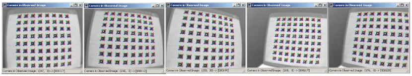
Figure 1: Five images of the model plane with the extracted corners (indicated by cross) for the desktop camera.

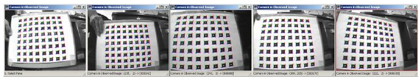
Figure 2: Five images of the model plane with the extracted corners (indicated by cross) for the ODIS camera.

From Tables II, III, and IV, it is observed that the final value of $J$ of model₃ is always greater than that of model₁, but much smaller than that of model₂. The comparison between model₂ and model₃ might not be fair since the new model has one more coefficient and it is evident that each additional coefficient in the model tends to decrease the fitting residual. However, our main point is to emphasize that by adding a quadratic term in $\delta_{r}$, higher accuracy can be achieved without sacrificing the property of having analytical undistortion function.

A second look at the results reveals that for the camera used in [19], which has a small lens distortion, the advantage of model₃ over model₂ is not so significant. However, when the cameras are experiencing a severe distortion, the radial distortion model₃ gives a much better performance over model₂, as can be seen from Tables III and IV.

Remark III.1

Classical criteria that are used in the computer vision to assess the accuracy of calibration includes the radial distortion as one part inherently [4]. However, to our best knowledge, there is not a systematically quantitative and universally accepted criterion in the literature for performance comparisons among different radial distortion models. Due to this lack of criterion, in our work, the comparison is based on, but not restricted to, the fitting residual of the full-scale nonlinear optimization in (9).

Remark III.2

To make the results in this paper reproducible by other researchers for further investigation, we present the options we use for the nonlinear optimization: options = optimset(‘Display’, ‘iter’, ‘LargeScale’, ‘off’, ‘MaxFunEvals’, 8000, ‘TolX’, $10^{-5}$, ‘TolFun’, $10^{-5}$, ‘MaxIter’, 120). The raw data of the extracted feature locations in the image plane are also available [20].

TABLE II: Comparison of Distortion Models Using Public Images

Public Images
Model	$\#1$	$\#2$	$\#3$
$J$	144.8802	148.2789	145.6592
$\alpha$	832.4860	830.7425	833.6508
$\gamma$	0.2042	0.2166	0.2075
$u_{0}$	303.9605	303.9486	303.9847
$\beta$	832.5157	830.7983	833.6866
$v_{0}$	206.5811	206.5574	206.5553
$k_{1}$	-0.2286	-0.1984	-0.0215
$k_{2}$	0.1905	-	-0.1566

TABLE III: Comparison of Distortion Models Using Desktop Images

Desktop Images
Model	$\#1$	$\#2$	$\#3$
$J$	778.9767	904.6797	803.3074
$\alpha$	277.1449	275.5953	282.5642
$\gamma$	-0.5731	-0.6665	-0.6199
$u_{0}$	153.9882	158.2016	154.4913
$\beta$	270.5582	269.2301	275.9019
$v_{0}$	119.8105	121.5257	120.0924
$k_{1}$	-0.3435	-0.2765	-0.1067
$k_{2}$	0.1232	-	-0.1577

TABLE IV: Comparison of Distortion Models Using ODIS Images

ODIS Images
Model	$\#1$	$\#2$	$\#3$
$J$	840.2650	933.0981	851.2619
$\alpha$	260.7658	258.3193	266.0850
$\gamma$	-0.2741	-0.5165	-0.3677
$u_{0}$	140.0581	137.2150	139.9198
$\beta$	255.1489	252.6856	260.3133
$v_{0}$	113.1727	115.9302	113.2412
$k_{1}$	-0.3554	-0.2752	-0.1192
$k_{2}$	0.1633	-	-0.1365

IV Concluding Remarks

This paper proposes a new radial distortion model for camera calibration that belongs to the polynomial approximation category. The appealing part of this distortion model is that it preserves high accuracy together with an easy analytical undistortion formula. Performance comparisons are made between this new model with two other existing polynomial radial distortion models. Experiments results are presented showing that this distortion model is quite accurate and efficient especially when the actual distortion is significant.

References

- [1] Zhengyou Zhang, “Flexible camera calibration by viewing a plane from unknown orientation,” IEEE International Conference on Computer Vision, pp. 666–673, September 1999.
- [2] Frederic Devernay and Olivier Faugeras, “Straight lines have to be straight,” Machine Vision and Applications, vol. 13, no. 1, pp. 14–24, 2001.
- [3] Roger Y. Tsai, “A versatile camera calibration technique for high-accuracy 3D machine vision metrology using off-the-shelf TV cameras and lenses,” IEEE Journal of Robotics and Automation, vol. 3, no. 4, pp. 323–344, August 1987.
- [4] Juyang Weng, Paul Cohen, and Marc Herniou, “Camera calibration with distortion models and accuracy evaluation,” IEEE Transactions on Pattern Analysis and Machine Intelligence, vol. 14, no. 10, pp. 965–980, October 1992.
- [5] Reimar K. Lenz and Roger Y. Tsai, “Techniques for calibration of the scale factor and image center for high accuracy 3-D machine vision metrology,” IEEE Transactions on Pattern Analysis and Machine Intelligence, vol. 10, no. 5, pp. 713–720, September 1988.
- [6] Chester C Slama, Ed., Manual of Photogrammetry, American Society of Photogrammetry, fourth edition, 1980.
- [7] J. Heikkil and O. Silvn, “A four-step camera calibration procedure with implicit image correction,” in IEEE Computer Society Conference on Computer Vision and Pattern Recognition, San Juan, Puerto Rico, 1997, pp. 1106–1112.
- [8] Janne Heikkila and Olli Silven, “Calibration procedure for short focal length off-the-shelf CCD cameras,” in Proceedings of 13th International Conference on Pattern Recognition, Vienna, Austria, 1996, pp. 166–170.
- [9] G. Wei and S. Ma, “Implicit and explicit camera calibration: theory and experiments,” IEEE Transactions on Pattern Analysis and Machine Intelligence, vol. 16, no. 5, pp. 469–480, May 1994.
- [10] Charles Lee, Radial Undistortion and Calibration on An Image Array, Ph.D. thesis, MIT, 2000.
- [11] Janne Heikkila, “Geometric camera calibration using circular control points,” IEEE Transactions on Pattern Analysis and Machine Intelligence, vol. 22, no. 10, pp. 1066–1077, October 2000.
- [12] Toru Tamaki, Tsuyoshi Yamamura, and Noboru Ohnishi, “Correcting distortion of image by image registration,” in The 5th Asian Conference on Computer Vision, January 2002, pp. 521–526.
- [13] D.C. Brown, “Close-range camera calibration,” Photogrammetric Engineering, vol. 37, no. 8, pp. 855–866, 1971.
- [14] Hany. Farid and Alin C. Popescu, “Blind removal of lens distortion,” Journal of the Optical Society of America A, Optics, Image Science, and Vision, vol. 18, no. 9, pp. 2072–2078, September 2001.
- [15] Lili Ma, YangQuan Chen, and Kevin L. Moore, “Flexible camera calibration using a new analytical radial undistortion formula with application to mobile robot localization,” in IEEE International Symposium on Intelligent Control, Houston, USA, October 2003.
- [16] Toru Tamaki, Tsuyoshi Yamamura, and Noboru Ohnishi, “Unified approach to image distortion,” in International Conference on Pattern Recognition, August 2002, pp. 584–587.
- [17] Zhengyou Zhang, “On the epipolar geometry between two images with lens distortion,” in International Conference on Pattern Recognition, Vienna, August 1996, pp. 407–411.
- [18] Ben Tordoff, Active Control of Zoom for Computer Vision, Ph.D. thesis, University of Oxford, Robotics Research Group, Department of Engineering Science, 2002.
- [19] Zhengyou Zhang, “Experimental data and result for camera calibration,” Microsoft Research Technical Report, http://rese- arch.microsoft.com/~zhang/calib/, 1998.
- [20] Lili Ma, “Camera calibration: a USU implementation,” CSOIS Technical Report, ECE Department, Utah State University, http://cc.usu.edu/ lilima/, May, 2002.
- [21] “Cm3000-l29 color board camera (ODIS camera) specification sheet,” http://www.video-surveillance-hidden-spy -cameras.com/cm3000l29.htm.