Abstract

We present memory-efficient deterministic algorithms for constructing $\epsilon$-nets and $\epsilon$-approximations of streams of geometric data. Unlike probabilistic approaches, these deterministic samples provide guaranteed bounds on their approximation factors. We show how our deterministic samples can be used to answer approximate online iceberg geometric queries on data streams. We use these techniques to approximate several robust statistics of geometric data streams, including Tukey depth, simplicial depth, regression depth, the Thiel-Sen estimator, and the least median of squares. Our algorithms use only a polylogarithmic amount of memory, provided the desired approximation factors are inverse-polylogarithmic. We also include a lower bound for non-iceberg geometric queries.

1 Introduction

With the proliferation of streams of packets on the Internet, as well as data streaming from embedded systems, digital monitors, sensor networks, and scientific instruments, there is a need for new algorithms that can compute approximations or answer approximate queries on data streams. The main challenge in these contexts is that the data volumes are often much larger than the memory size of a typical computer. Thus, there is a considerable amount of interest in methods that can process data streams using limited memory (e.g., see recent surveys by Muthukrishnan [27] and Babcock [2]). The model we choose to work in is the so called Time Series model in which each time instant reveals a new element of the data stream “signal.”

A typical approach in data streaming algorithms is to maintain a random sample of the input data and perform computations on the sample with the hope that information about the sample can be used to infer properties of the entire set. Naturally, such inferences come with an associated probability that they are inaccurate. In this paper, we are interested in deterministically constructing samples of a data stream that have guaranteed approximation properties for the original set. Moreover, because of the limited memory restriction of data streaming applications, we are interested in deterministic samples that can be constructed using space that is polylogarithmic in the data stream’s length.

In addition, because much of the streaming data is coming from sensors and scientific instruments, we are interested in this paper in studying streaming algorithms for geometric data. Such data could include multi-dimensional points in the color space of astrophysical data or two-dimensional lines defined by a point-line duality of a stream of points in the plane. Of particular interest, then, is data streaming algorithms for constructing $\epsilon$-nets and $\epsilon$-approximations, which are general structures developed in the computational geometry literature for deterministically sampling geometric data. Indeed, $\epsilon$-nets and $\epsilon$-approximations are developed in a very general context of bounded-dimensional range spaces, where we are given a ground set and a polynomial-sized family of ranges on that set (which constitute the queries or sampling statistics we are interested in). Hence, results for constructing such deterministic samples should have a considerable number of applications.

1.1 Related work on Streaming Algorithms

Data streaming problems have engendered a large amount of interest among the algorithms community over the last few years. For a comprehensive survey of the work done so far and some interesting directions for the future, the reader is referred to Muthukrishnan’s work [27]. An earlier survey by Babcock et. al. [2] explores the issues arising in building data stream systems.

We are not familiar with any previous work for constructing $\epsilon$-nets or $\epsilon$-approximations in streaming models, although these structures have been extensively studied in full-memory contexts (e.g., see the chapter by Matoušek [26]). The closest previous work is done in the iceberg query [9] framework of Manku and Motwani [22], who provide $1+\epsilon$ approximations for the frequency counts of items in a data stream that occur more than $\epsilon N$ times (which are the so-called “icebergs”). Similarly, algorithms for computing the quantiles of a data stream have been given by Greenwald and Khanna [12] guaranteeing a precision of $\epsilon N$, which is similar to the guarantees that are provided by $\epsilon$-approximations, while using $O(\frac{1}{\epsilon}\log\epsilon N)$ space. This limitation of an additive $\epsilon N$ error in every quantile is overcome by Gupta and Zane [13]. The latter’s method provides relative error for all quantiles but uses $O(\log^{2}N/\epsilon^{3})$ space and requires knowledge of an upper bound on the stream size.

The first geometric problem to be studied in the streaming model was that of finding the diameter of a set of points. Feigenbaum, Kannan and Zhang [10] gave an $O(1/\epsilon)$ space algorithm for computing the diameter of points in two dimensions in the streaming model and a $O(\frac{1}{\epsilon^{3/2}}\cdot\log^{3}N(\log R+\log\log N+\log(\frac{1}{\epsilon})))$ space algorithm for computing it in the sliding window model where $R$ is the maximum, over all windows, of the ratio of the diameter to the distance between the closest two points in the window. Indyk [16] gave a streaming algorithm which maintains a $c$-approximate diameter of points in $d$ dimensions using $O(dn^{1/(c^{2}-1)})$ space taking $O(dn^{1/(c^{2}-1)})$ time per new point, for $c>\sqrt{2}$.

Cormode and Muthukrishnan generalized the exponential histograms used on single dimensional data sets in earlier works on streaming algorithms [7, 19] and defined radial histograms [6], which allowed them to give a $O(1+\epsilon)$ approximation to the diameter using $O(1/\epsilon)$ space. They were also able to use these structures to approximate convex hulls in the sense that no point in the input stream is more than $\epsilon D$ outside the approximate hull, where $D$ is the diamter of the point set. Constructing an approximate hull takes them $O(q/\epsilon)$ space. Hershberger and Suri [15] improve this to give a sampling-based algorithm for approximating the convex hull of a streaming point set, showing how to maintain an adaptive sample of at most $2r$ points such that the distance between the hull of their sample and the true convex hull is $O(D/r^{2})$, where $D$ is the current diameter of the sample. Some of the other geometric problems that have been studied in a streaming model include minimum spanning tree and minimum weight matching [17] and certain facility location and nearest neighbour kind of queries [6].

1.2 Our Results

In this paper, we present memory-efficient deterministic algorithms for constructing $\epsilon$-nets and $\epsilon$-approximations of streams of geometric data. Our algorithms use a polylogarithmic amount of memory, provided $\epsilon$ is at least inverse-polylogarithmic. As mentioned above, $\epsilon$-nets and $\epsilon$-approximations are of interest in their own right and have many applications in computational geometry. We show how our deterministic samples can be used to answer online iceberg geometric queries on data streams, such as in multi-dimensional iceberg range searching. Because the information typically of interest from data streams is statistical, we focus in this paper primarily on the use of $\epsilon$-nets and $\epsilon$-approximations to compute approximations to several robust statistics of geometric data streams, including Tukey depth, simplicial depth, regression depth, the Thiel-Sen estimator, and the least median of squares. Thus, we additionally give polylogarithmic-space data streaming algorithms for computing approximations to these statistics. We also include a lower bound for non-iceberg range queries in data streams.

2 Preliminaries on $\epsilon$-Nets and $\epsilon$-Approximations

In this section we recap certain aspects of $\epsilon$-Nets and $\epsilon$-approximations [34, 26], which are part of a general framework for modelling a number of interesting problems in computational geometry and derandomizing divide-and-conquer type algorithms.

A range space is a set system, i.e., a pair $\Sigma=(X,\mathcal{R})$, where $X$ is a set and $\mathcal{R}$ is a set of subsets of $X$. We call the elements of $\mathcal{R}$ the ranges of $\Sigma$, as $\mathcal{R}$ is typically defined in terms of some well structured geometry. If $Y$ is a subset of $X$, we denote by $\mathcal{R}|_{Y}$ the set system induced by $\mathcal{R}$ on $Y$, i.e., $\{R\cap Y|R\in\mathcal{R}\}$.

We say a subset $Y\subseteq X$ is shattered if every possible subset of $Y$ is induced by $\mathcal{R}$, i.e., if $\mathcal{R}|_{Y}=2^{Y}$. The VC-dimension of $\Sigma$ is the maximum size of a shattered subset of $X$. If there are shattered subsets of any size, then the VC-dimension is infinite. A related and simpler notion is the scaffold dimension [11] of $\Sigma$. It is based on the notion of the shatter function $\pi_{\mathcal{R}}(m)$, which we define as the maximum possible number of sets in a subsystem of $\Sigma$ induced by an $m$-sized subset of $X$. In other words, it is the $\sup\{|R|_{Y}|:Y\subseteq X,|Y|=m\}$. We now define the scaffold dimension of $(X,\mathcal{R})$ as the infimum of all numbers $d$ such that $\pi_{\mathcal{R}}(m)$ is $O(m^{d})$. It turns out that the shatter function of a set system of VC-dimension $d^{\prime}$ is bounded by $\binom{m}{0}+\binom{m}{1}+\cdots+\binom{m}{d^{\prime}}=\Theta(m^{d^{\prime}})$ [31, 34]. Thus the scaffold dimension is always at most the VC-dimension. Conversely, if the scaffold dimension is bounded by a constant, the VC-dimension too is bounded by a constant. There are, however, many natural geometric set systems of scaffold dimension strictly smaller than the VC-dimension; for instance, the scaffold dimension of a set system defined by halfplanes in the plane is 2, while the VC-dimension is 3. In the rest of the paper, we will always refer to the scaffold dimension of a set system. In addition, we consider only those set systems whose scaffold dimensions are bounded by a constant.

We are now ready to define $\epsilon$-nets and $\epsilon$-approximations. A subset $S\subseteq X$ is an $\epsilon$-net for $(X,\mathcal{R})$ provided that $S\cap R\not=\emptyset$ for every $R\in\mathcal{R}$ with $|R|/|X|<\epsilon$. A subset $A\subseteq X$ is an $\epsilon$-approximation for $(X,\mathcal{R})$ provided that

$$\left|\frac{|A\cap R|}{|A|}-\frac{|X\cap R|}{|X|}\right|\leq\epsilon$$ (1)

for every set $R\in\mathcal{R}$. Note that every $\epsilon$-approximation is automatically an $\epsilon$-net, but the converse need not be true. A remarkable property about set systems of scaffold dimension $d$ is that, for any $\epsilon\in[0,1)$, they admit an $\epsilon$-approximation whose size depends only on $d$ and $\epsilon$, not on the size of $X$. The first basic result in this vein is the following lemma.

Lemma 2.1

For any set system $(X,\mathcal{R})$, with a finite $X$, and a scaffold dimension at most $d$, where $d\geq 1$, there exists, for any $\epsilon\in[0,1]$, an $\epsilon$-net of size at most $C_{1}\epsilon^{-1}\lg(\epsilon^{-1})$, and an $\epsilon$-approximation of size at most $C_{2}\epsilon^{-2}\lg(\epsilon^{-1})$. Here $C_{1},C_{2}$ depend on only $d$.

Note that, in general, the $\lg(\epsilon^{-1})$ factor cannot be removed from the bound.

Matoušek [25] gave a deterministic algorithm for efficiently computing small sized $\epsilon$-approximations (and thereby, $\epsilon$-nets) for set systems with constant-bounded scaffold dimensions. Such an algorithm needs that the set system to be given in a form more “compact” than simply the listing of the elements in each set. For this we assume the existence of a subsystem oracle, i.e. an algorithm (depending on the specific geometric application) that, given any subset $Y\subseteq X$, lists all sets of $\mathcal{R}|_{Y}$. We say that the subsystem oracle is of dimension at most $d$ if it lists all sets in time $O(|Y|^{d+1})$. This corresponds to the scaffold dimension; the maximum number of sets in $\mathcal{R}|_{Y}$ is $\pi_{\mathcal{R}}(|Y|)$, and the “$+1$” in the exponent accounts for the fact that each output set is given by a list of size up to $|Y|$. Matoušek’s result is summarized by the following lemma.

Lemma 2.2

Let $(X,\mathcal{R})$ be a set system with a subsystem oracle of dimension $d$, where $d$ is a constant. Given any $\epsilon\in[0,1)$, we can compute an $\epsilon$-approximation of size $O(\epsilon^{-2}\lg(\epsilon^{-1}))$ and an $\epsilon$-net of size $O(\epsilon^{-1}\lg(\epsilon^{-1}))$ in time $O(|X|\epsilon^{-2d}\lg^{d}(e^{-1}))$.

We shall use the algorithm above as a sub-routine for our streaming algorithm for $\epsilon$-approximations (see Section 4). It is based on two observations that we state below. They correspond to two basic operations of our algorithm, the merge step and the reduce step. Many algorithms for computing $\epsilon$-approximations (certainly the one Matoušek gave, and the one we shall give) start by partitioning $X$ into small pieces, and then essentially alternate between the two steps until they get the desired approximation.

Observation 2.3 (Merge Step)

Let $X_{1},\ldots,X_{m}\subseteq X$ be disjoint subsets of equal cardinality and let $A_{i}$ be an $\epsilon$-approximation of cardinality $b$ for $(X_{i},\mathcal{R}|_{X_{i}}),i=1,\ldots,m$. Then $A_{1}\cup\ldots\cup A_{m}$ is an $\epsilon$-approximation for the subsystem induced by $\mathcal{R}$ on $X_{i}\cup\ldots\cup X_{m}$.

Observation 2.4 (Reduce Step)

Let $A$ be an $\epsilon$-approximation for $(X,\mathcal{R})$ and let $A^{\prime}$ be a $\delta$-approximation for $(A,\mathcal{R}|_{A})$. Then $A^{\prime}$ is an $(\epsilon+\delta)$-approximation for $(X,\mathcal{R})$.

Before we end this preliminary section, we state the following extension to Lemma 2.2. This, too, was given by Matoušek [25].

Lemma 2.5

Let $X$ be a finite set equipped by a probabilistic measure $\mu$ (given by a table) and let $\Sigma=(X,\mathcal{R})$ be a range space satisfying the assumptions of Lemma 2.2. Then an $\epsilon$-approximation for $\Sigma$ with respect to the measure $\mu$ can be computed with the same asymptotic efficiency in the running time and size of the $\epsilon$-approximation in the case of uniform measure in Lemma 2.2.

When $X$ is associated with a probabilistic measure $\mu$, an $\epsilon$-approximation of $(X,\mathcal{R})$ is a multi-set $A$ such that

$$\left|\frac{|A\cap R|}{|A|}-\frac{\mu(X\cap R)}{\mu(X)}\right|\leq\epsilon$$

for every $R\in\mathcal{R}$.

3 Some Additional Extensions for Weighted Sets

While the extensions described above are useful in our context, we nevertheless need some further generalizations, which will be useful in the data streaming model. In particular, we need to generalize Observation 2.3 to a weighted case. This allows us to merge $\epsilon$-approximations of different sizes and for sets of different cardinalities. To the best of our knowledge, this is the first time such an observation is being made. Note that in the un-weighted case, for an $\epsilon$-approximation $A$ for $(X,\mathcal{R})$, each element in $A$ “represents” $|X|/|A|$ elements in $X$. This is easy to see if we write Requirement 1 in the following form

$$\left||A\cap R|\frac{|X|}{|A|}-|X\cap R|\right|\leq\epsilon|X|$$

Now, instead of having an element p in the $\epsilon$-approximation $A$ represent the same number of elements in $X$, we can assign it a weight $\gamma(p)$ equal to the number of elements in $X$ that it represents. In this generalized scenario, a subset $A\subseteq X$, is a weighted $\epsilon$-approximation for $(X,\mathcal{R})$ provided that

$$\left|\sum_{p\in A\cap R}\gamma(p)-|X\cap R|\right|\leq\epsilon|X|.$$

We are now ready to state our observation related to weighted merging.

Observation 3.1 (Weighted Merge Step)

Let $X_{1},\ldots,X_{m}\subseteq X$ be disjoint subsets (of cardinalities not necessarily the same) and let $A_{i}$ be a weighted $\epsilon$-approximation of $(X_{i},\mathcal{R}|_{X_{i}}),i=1,\ldots,m$. Then $A_{1}\cup\ldots\cup A_{m}$ is a weighted $\epsilon$-approximation for the subsystem induced by $\mathcal{R}$ on $X_{i}\cup\ldots\cup X_{m}$, where the weights on the points remain as they were.

4 Computing $\epsilon$-Approximations in Geometric Streams

Let $x_{1},\ldots,x_{n},\ldots$ be a stream of geometric objects in the time series model. Let $X$ be the set of all the objects in the stream that have arrived till now. Let $\mathcal{R}$ be a set of ranges defined on $X$, and $\Sigma=(X,\mathcal{R})$ be the current range space. In addition, let $d$, where $d$ is a constant, be the scaffold dimension of $\Sigma$.

We present an algorithm which computes an $\epsilon$-approximation to $(X,\mathcal{R})$, given any $\epsilon\in[0,1)$. Our algorithm maintains a polylogarithmic-sized data structure from which it computes this $\epsilon$-approximation. Additionally, it takes polylogarithmic time to update this structure on the arrival of a new item in the stream.

The $\epsilon$-approximation our algorithm produces is asymptotically equal in size to that produced in the static model (see Lemma 2.2). Interestingly, our algorithm does not need to know the value of $n$ in advance. Our algorithm simulates the divide-and-conquer approach of the static algorithm in a bottom up fashion. We now outline how this is done.

We begin by imposing a hierarchy of groupings onto the stream: define canonical sets $S_{j,k}$ as $\{x_{i}|j2^{k}\leq i<(j+1)2^{k}\}$ for $j,k\geq 0$. Canonical sets are inter-related through a natural tree hierarchy. The children of set $S_{j,k}$, $k\geq 1$, are the canonical sets $S_{2j,k-1}$ and $S_{2j+1,k-1}$. We say that a canonical set $S_{j,k}$ becomes available when the last element in it, i.e., $x_{(j+1)2^{k}-1}$, arrives. A maximal canonical set is one that is available but whose parent is not yet available. Observe that when $x_{n}$ arrives, there are at most $\lg n$ maximal canonical sets. Also, the union of all the maximal canonical sets is the set $X$ of all elements that have arrived till now.

We use the following building blocks.

• $\epsilon$-approx(): An algorithm for deterministically computing $\epsilon$-approximation with small size (see Lemma 2.2.)

• weighted_$\epsilon$-approx(): An algorithm for deterministically computing $\epsilon$-approximations of weighted items (see Lemma 2.5.)

Note that we cannot afford to use $\epsilon$-approx() on an input that is larger than logarithmic, as otherwise we will not remain within our space and time bounds.

Our algorithm, we call it $\epsilon$-stream_approx(), follows the basic merge and reduce technique [26] for constructing $\epsilon$-approximations. To follow this technique we need to use a sequence $w_{1},\ldots,w_{u},\ldots$ with the property that $W\triangleq\sum_{u=1}^{\infty}w_{u}=O(1)$. Here we shall use $w_{i}=i^{-1-c}$, for some $c>0$.

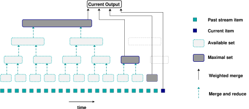
Figure 1: Schematic: Computing an $\epsilon$-approximation of a data stream

At a high level the algorithm is as follows (see Figure 1): At every stage, the algorithm stores a $\delta$-approximation for all available maximal canonical sets, where $\delta$ varies with the set, but is always at most $\epsilon/2$. Let $A_{j,k}$ be such an approximation for $S_{j,k}$. This $\delta$-approximation is constructed through merging the approximations $A_{2j,k-1}$ and $A_{2j+1,k-1}$ which were earlier computed for $S_{j,k}$’s two children.

The $\epsilon$-approximation of the set $X$ at any point, the stream output, is determined by weighted merging. Each element $p\in A_{j,k}$ is assigned a weight $\gamma(p)=|S_{j,k}|/|A_{j,k}|$ for this purpose. As it happens, once a weight is assigned to an object, we don’t ever need to change it.

We are now ready to formally specify $\epsilon$-stream_approx(). Figure 2 contains the specification. Assume that $A_{j,0}$ is the element itself in the singleton set $S_{j,0}$.

$\epsilon$-stream_approx() When the next element $x_{n}$ in the stream arrives For each canonical set $S_{j,k}$ that becomes available, taken in the order of increasing $k$, where $k\geq 1$ /* Combine approximations of its children using (un-weighted) merge to get approximation for the parent */ $B\leftarrow A_{2j,k-1}\cup A_{2j+1,k-1}.$ /* Reduce the size of the approximation */ $A_{j,k}\leftarrow$ $(\epsilon/2\cdot w_{k}/W)$-approximation of $B$ using $\epsilon$-approx(). /* Assign weights to elements */ For all $p\in A_{j,k}$: $\gamma(p)\leftarrow|S_{j,k}|/|A_{j,k}|.$ /* Combine approximations of maximal canonical sets using weighted merge to get approximation for the stream */ $A^{\prime}\leftarrow\bigcup_{\mbox{$S_{j,k}$ is available}}A_{j,k}$. Each element in $A^{\prime}$ retains its weight from its orginal $A_{j,k}$. /* Reduce the size of the approximation */ $A\leftarrow$ $(\epsilon/2)$-approximation of $A^{\prime}$ using weighted_$\epsilon$-approx(). Output $A$.

Figure 2: Algorithm for computing an $\epsilon$-approximation of a geometric stream.

Correctness, Space, and Time.

Observations 2.3 and 2.4 imply that $A_{i,j}$ is a $\delta$-approximation for $S_{j,k}$, where

$$\delta\leq\sum_{u=1}^{k}\frac{\epsilon}{2}\cdot\frac{w_{u}}{W}<\frac{\epsilon}{2}.$$

Together with Observation 3.1, this implies that $A^{\prime}$ is a weighted $(\epsilon/2)$-approximation for the set $X$ of elements in the stream. Now bring in the properties of weighted_$\epsilon$-approx() and another application of Observation 2.4 to see that $A$ is indeed an $\epsilon$-approximation of $(X,\mathcal{R})$.

The data structure needs to store just the ‘$A_{j,k}$’s; all other sets are intermediate results that can be discarded. Lemma 2.2 implies that the size of $A_{j,k}$, is $O((\epsilon\cdot w_{k})^{-2}\lg((\epsilon\cdot w_{k})^{-1}))$; remember that the size is determined by just the last reduction step. Denote the size of largest such set, i.e., $A_{j,\lg n}$, by $s=s(n,\epsilon^{-1})$, which is $O(\lg^{2+2c}n\cdot\epsilon^{-2}\cdot(\lg\lg n-\lg\epsilon))$. Note that $s$ is also an upper bound for the size of the input to $\epsilon$-approx().

Consider the space and time requirements. These are dominated by the requirements for weighted_$\epsilon$-approx(). The input to weighted_$\epsilon$-approx()is $O(\lg n\cdot s)$. Lemma 2.5 implies that the space and time requiments for $\epsilon$-stream_approx() are $O(\lg^{3+2c}n\cdot e^{-2d-2}\lg(e^{-1})\cdot(\lg\lg n-\lg\epsilon))$.

5 Applications

$\epsilon$-Nets and $\epsilon$-approximations have a number of applications in computational geometry, and even other areas like learning theory — see, e.g., [24]. Many of the problems in these have streaming versions. One basic application is range counting. In this, we are given a set $S$ of $n$ points in $\mathbb{R}^{d}$, and a family $\mathcal{R}$ (the ranges) of subsets of $\mathbb{R}^{d}$. Each query consists of a range $R\in\mathcal{R}$ and asks for the number of points in it. Typical range families are axes-orthogonal ranges, spherical ranges (proximity queries), and simplical ranges. The corresponding range spaces for these all have a bounded scaffold dimension. In the streaming version, the point set $S$ comes as a continuous stream, interspersed with queries. It is easy to see how our algorithm would work here: use $\epsilon$-stream_approx() to maintain an $\epsilon$-approximation $A$ of the current $(S,\mathcal{R})$. When queried with range $R\in\mathcal{R}$, output $|A\cap R|\cdot n/|A|$. This is within an additive $\epsilon n$ of the true value; this is akin to the iceberg queries mentioned earlier.

The above technique has implications in a lot of specific applications. To get a flavor of this, we delve deeper into the specific area of robust statistic in the next few paragraphs.

5.1 Robust Statistics

Robust statistics concerns the study of statistical estimators that can tolerate high numbers of outliers, while maintaining an accuracy of estimation that depends only on the remaining uncorrupted data points. In contrast, ordinary least squares estimators, while trivial to compute even in the streaming model, can be forced to produce estimates that are arbitrarily far from the correct model even in the presence of a single outlier. The number of outliers that an estimator can tolerate while preserving its accuracy is called its breakdown point; in general, methods with high breakdown points are preferred but other criteria are also important including statistical efficiency (number of samples needed to achieve a given accuracy) and computational efficiency (amount of time it takes to compute a given estimate from a set of samples). Many robust statistical methods also have the advantage of being non-parametric, not requiring the statistician to produce a prior probability distribution or other arbitrary parameters before producing a fit. The paradigmatic example of a robust statistic is the median of one-dimensional data, which, unlike the mean, is robust with a breakdown point of $\frac{1}{2}$. Much research on streaming algorithms has gone into methods for maintaining approximate medians or more general quantiles [12], and we would like to find similar methods for higher dimensional statistics.

Two of the critical problems studied in robust statistics are location (finding a central point in a cloud of data points) and regression (fitting the data to a model in which a dependent variable or variables is a linear function of the independent variables). Many methods in this area are based on various concepts of depth, which measures the quality of fit of an estimate. It is natural to seek the estimate maximizing the depth, but it is also of importance to be able to compute depths of non-optimal estimates, in order to form depth contours that produce a center-outward ordering of the data.

For many of these robust statistical methods, a computationally efficient streaming approximation to the depth measure can be obtained from an $\epsilon$-approximation of the sample data. The deepest fit can be approximated by a deepest fit to the $\epsilon$-approximation, and this approximate fit often has similar breakdown point properties to the non-approximate fit on which it is based. We describe below several of the methods to which this technique applies:

Tukey Depth.

This quantity [8] measures the quality of fit of a center, as the minimum proportion of sample points among all halfspaces that contain the center. The Tukey depth of a point can be computed in time $O(n^{d}\log n)$, where $n$ denotes the number of sample points [30]. The Tukey median is the point of maximum depth. It is known that any Tukey median has depth at least $1/(d+1)$, and the breakdown point of the Tukey median as an estimate of location is also $1/(d+1)$. There are known static algorithms for finding Tukey medians, or other points of high depth, in two or three dimensions [18, 20, 23], but in higher dimensions only inefficient linear-programming based exact solutions are known and it is necessary to resort to more efficient approximation algorithms [5].

Since the Tukey depth is based on counting points in halfspaces, it can be approximated using $\epsilon$-approximations for halfspace ranges [5]: the depth of a point within an $\epsilon$-approximation of a sample is within an additive error of $\epsilon$ of its depth in the original sample data. In particular, the Tukey median of an $\epsilon$-approximation has depth within $\epsilon$ of that of the true Tukey median. The breakdown point of this approximate Tukey median is $1/(d+1)-\epsilon$. Thus, by using our streaming $\epsilon$-approximation algorithm, we can efficiently maintain not only an approximate Tukey median of the data set, but also a space-efficient data structure from which we can compute accurate approximations of the Tukey depth of any point.

Simplicial Depth.

This is another measure of quality of fit for location, introduced by Liu [21]. The simplicial depth of a fit point is defined to be the proportion of simplices, among all the $n\choose d+1$ simplices formed by convex hulls of $(d+1)$-tuples of sample points, that contain the fit point. Equivalently, it is the probability that a randomly chosen $(d+1)$-tuple contains the fit point in its convex hull. As we now argue, for points in the plane, the simplicial depth in a sample set is accurately approximated by the simplicial depth of an $\epsilon$-approximation for wedge ranges (that is, ranges formed by intersecting two halfplanes). Therefore, as for Tukey depth, we can answer approximate depth queries and maintain an approximate deepest point in a space-efficient manner for streaming data.

Let $\delta$ be a value to be determined later and imagine the following process for measuring approximately the simplicial depth of a fit point: first, let $L$ be a set of $1/\delta$ lines through the fit point, partitioning the plane into $2/\delta$ wedges having the fit point as a common apex, with at most a $\delta$ fraction of the sample points in any wedge. Let $e_{1}$ be the proportion of triangles, determined by three input points, that are not all on one side of one of a line in $L$. Then $e_{1}$ is an overestimate of the simplicial depth, but the amount by which it overestimates the depth is $O(\delta)$: the only triangles incorrectly included in the estimate are ones that have two points in opposite wedges, there are $O(\delta^{2}n^{3})$ such triangles per pair of opposite wedges, and $O(1/\delta)$ such pairs. Next, let $e_{2}$ be the proportion of triangles, determined by three points in an $\epsilon$-approximation of the sample, that are not all on one side of a line in $L$. For the same reasons as before, $e_{2}$ is within $O(\delta)$ of the simplicial depth for the $\epsilon$-approximation. Further, $e_{1}$ and $e_{2}$ are within $O(\epsilon/\delta)$ of each other:

$$e_{1}=1-\sum_{i}{{w_{i}\choose 3}+{w_{i}\choose 2}(h_{i}-w_{i})+w_{i}{h_{i}-w_{i}\choose 2}\over{n\choose 3}},$$

where $w_{i}$ is the number of sample points in the $i$th wedge and $h_{i}$ is the number of sample points in the halfplane containing the $i$th wedge on its counterclockwise boundary. Each term in the sum is approximated within $O(\epsilon)$ by the corresponding term where $w_{i}$ and $h_{i}$ are replaced by numbers of points in the $\epsilon$-approximation, and there are $O(1/\delta)$ terms, so the total difference between $e_{1}$ and $e_{2}$ is $O(\epsilon/\delta)$. Putting together the errors in going from the original simplicial depth to $e_{1}$ to $e_{2}$ to the simplicial depth of the approximation, and setting $\delta=\sqrt{\epsilon}$, we see that the $\epsilon$-approximation approximates the simplicial depth to within $O(\sqrt{\epsilon})$.

As far as we are aware, this deterministic $\epsilon$-approximation based method for approximating simplicial depth is novel even for static, non-streaming data, although it is trivial to approximate simplicial depth randomly in the static case by sampling triangles. It seems likely that similar deterministic and streaming approximation guarantees, with worse dependence on $\epsilon$, can be shown to hold also in higher dimensions.

Regression Depth.

This statistic was introduced by Rousseeuw and Hubert [28] as a measure of the quality of fit of a regression hyperplane. It is defined as being the minimum proportion of sample points that can be removed to turn the fit plane into a nonfit, that is, a hyperplane combinatorially equivalent to a vertical hyperplane. Amenta et al. [1] showed that, like Tukey depth, for regression depth a fit always exists with depth at least $1/(d+1)$, and the breakdown point of the maximum-depth fit is $1/(d+1)$. Their proof technique shows that the regression depth of a query hyperplane can be measured by performing a certain projective transformation of the space containing the sample points, and measuring the Tukey depth of a certain point in the transformed space. Due to the transformation, a halfspace in the transformed space may correspond to a double wedge (symmetric difference of two halfspaces) in the original space. Therefore, the same $\epsilon$-approximation technique used for Tukey depth, but with double wedge ranges, also applies to regression depth, and lets us compute depths and maintain an approximate deepest fit with high breakdown point for streaming data. Bern and Eppstein [3] generalized regression depth to the context of multivariate regression, in which the sample data have more than one dependent variable; in their definition, the depth of a fit is the minimum proportion of sample data contained in any double wedge, one boundary of which contains the fit and the other of which is parallel to the dependent coordinate axes; this is again well approximated by $\epsilon$-approximations for double wedge ranges.

The Thiel-Sen Estimator.

This estimator [32, 33] is a method for two-dimensional linear regression, in which one first finds the median among all $n\choose 2$ slopes determined by the lines through pairs of sample points, and then selects a regression line having that median slope and bisecting the sample set. It has a breakdown point of $1-\sqrt{1/2}\approx 0.293$. This has long been a testbed for geometric optimization algorithms, and several $O(n\log n)$ time static algorithms for it are known, among them one based on using $\epsilon$-cuttings in a prune-and-search technique [4]. However these algorithms seem to require repeatedly scanning the data in a way that is unavailable to a streaming algorithm. Instead, we apply an approximation technique very similar to that for simplicial depth, above.

To begin with, suppose that we are given a query slope $s$, and must determine the approximate position of $s$ within the sorted sequence of slopes, normalized by dividing the position by $n\choose 2$. This can be solved exactly by a reduction to computing the number of inversions in a permutation, but we are interested in approximations that can be computed by a streaming algorithm that does not know $s$ in advance. To do this, let $\delta$ be a parameter to be determined later, and imagine subdividing the sample points into a grid by $O(1/\delta)$ lines that are vertical and parallel to $s$, in such a way that at most a $\delta$ proportion of the points lie in the slab between any two adjacent parallel grid lines. Let $e_{1}$ be an estimate of the position of $s$, formed by summing up the normalized number of pairs of points that form a line with lower slope than $s$ and that are in a pair of grid cells that are separated both by a vertical line of the grid and by a line parallel to $s$ from the grid. Then $e_{1}$ is within $O(\delta)$ of the true position of $s$ since the only lines through a given point that are omitted from the count are the ones where the other point determining the line is in one of the two slabs containing $s$, and $e_{1}$ can be expressed as a sum with $O(\delta^{-2})$ terms, each term being a product of the number of points in two parallelograms. Let $e_{2}$ be a similar normalized sum, with the number of sample points in each parallelogram replaced by the number of points of an $\epsilon$-approximation for parallelogram ranges, and let $e_{3}$ be the normalized position of $s$ within the set of lines determined by pairs of points from the $\epsilon$-approximation. Then $e_{1}$ differs from $e_{2}$ by $O(\epsilon\delta^{-2})$ and $e_{2}$ differs from $e_{3}$ by $O(\delta+\epsilon\delta^{-1})$. Therefore, the overall error caused by using $e_{3}$ as our approximation to the position of $s$ is $O(\delta+\epsilon\delta^{-2})$. Setting $\delta=\epsilon^{1/3}$ makes this total error equal $O(\epsilon^{1/3})$.

To compute an approximate Thiel-Sen estimator, we use the same $\epsilon$-approximation for parallelograms, compute the median slope among pairs of points from the approximation, and then find a line with that median slope bisecting the approximation. The resulting line has slope with a normalized position within $O(\epsilon^{1/3})$ of the median slope, partitions the sample points within $\epsilon$ of exact bisection, and has a breakdown point of $1-\sqrt{1/2}-O(\epsilon^{1/3})$.

Least Median of Squares (LMS).

These methods [29] in robust statistics seek a fit that minimizes the median residual value separating the fit from the sample points. This is not a depth-based criterion, but it leads to fits which are highly robust against outliers. For location problems, the least median of squares fit is the center of the minimum radius sphere that contains at least half of the sample data [14]. It has a breakdown point of $\frac{1}{2}$: if fewer than half the sample data points are outliers, then the sphere defining the LMS fit has smaller radius than the circumsphere of the non-outliers, and it contains at least one non-outlier, so its center must be an accurate fit. Clearly, this is the best breakdown point possible for any location method. The natural type of $\epsilon$-approximation to use for this problem is one with balls as its ranges. If we form the LMS fit of such an $\epsilon$-approximation, the result may not be robust. Instead, we approximate the LMS fit by finding the center of the minimum radius sphere that contains at least a $\frac{1}{2}+\epsilon$ proportion of the points in the $\epsilon$-approximation. Such a sphere must therefore contain at least half of the sample data, and has a radius at least as small as the smallest sphere containing at least a $\frac{1}{2}+2\epsilon$ fraction of the sample data. It is robust with a breakdown point of $\frac{1}{2}-2\epsilon$.

The same LMS approach can also be applied to regression problems. The least median of squares regression hyperplane can be defined as the central hyperplane in a slab bounded by two parallel hyperplanes, with minimum vertical separation between them, that contains at least half of the sample data; again this is robust with a breakdown point of $\frac{1}{2}$. As above, we can use an $\epsilon$-approximation, with slab ranges, and find the slab with minimum vertical separation containing a $\frac{1}{2}+\epsilon$ fraction of the $\epsilon$-approximation points, to produce an approximate LMS fit with breakdown point $\frac{1}{2}-2\epsilon$.

6 A Lower Bound on Range Counting

We provide a simple lower bound on the space required to count approximately the number of items in a range that is not necessarily an iceberg. When we say that an algorithm $f$-approximates the range counting problem we mean that if a given range contains $l$ points, the algorithm gives us an answer which lies between $l/f$ and $l\cdot f$.

The bound is stated in terms of two-sided ranges: a point $(x,y)$ is said to belong to the two sided range located at $(p,q)$ if $x\geq p$ and $y\geq q$.

Theorem 6.1

Any $f$-approximate algorithm to the two-sided range counting problem must use space $\Omega(n/f^{2})$.

We begin by assuming there is an algorithm $A$ which gives an $f$ approximation to the two-sided range counting problem for a stream of points in two dimensions. Further we assume that this algorithm uses space $o(n/f^{2})$.

Now consider a set of $n$ points which are grouped in $n/f^{2}$ equally sized groups, we call them $G_{i}$, where $1\leq i\leq n/f^{2}$, in the following way:

• Each point in $G_{i}$ has the same $x$ coordinate, we call it $x_{i}$. Additionally, we require $x_{i}>x_{i-1}$.

• All the points in $G_{i}$ have $y$ coordinates closely clustered at a given value, we call it $y_{i}$. Formally, for every $p_{j}\in G_{i}$, we say that $0\leq y(p_{j})-y_{i}<1/2$.

• Every point $p_{j}\in G_{i}$ has $y$-coordinate strictly smaller than the $y$-coordinates of all the points in $G_{i-1}$.

• Each group $i$ has an additional point $q_{i}=(x_{i}+\epsilon,y_{i}+\epsilon)$, for some $\epsilon<1/2$, associated with it.

Note that this family of input sequences has the property that a two-sided query made at $(x_{i},y_{i})$ should return a count of $f^{2}+1$ and one made at $(x_{i}+\frac{\epsilon}{2},y_{i}+\frac{\epsilon}{2})$ should return a count of 1. This radical change in the counts will not occur between two such queries at any point which is not actually $(x_{i},y_{i})$ for some value of $i$. As an extension to this simple observation, we note that if all the $x_{i}$s and $y_{i}$s are chosen out of the integers $1,2,\ldots n$, it is possible to extract the exact values of all the $x_{i}$ with exactly $2n^{2}$ queries.

Let us see if the algorithm $A$ can be the query mechanism which we can deploy to this end. Since $A$ is an $f$ approximation, it should return a value of at most $f$ at $(x_{i}+\frac{\epsilon}{2},y_{i}+\frac{\epsilon}{2})$ and a value between $f+1/f$ and $f^{3}+f$ at $(x_{i},y_{i})$. This means that $A$ can indeed act as the oracle which identifies the locations of the groups in our set.

Hence, using $A$ as a subroutine we can extract $\theta(n/f^{2})$ information about the input set. This contradicts the assumption that $A$ uses space $o(n/f^{2})$. $\sqcap$$\sqcup$

Seen in the context of streaming algorithms, Theorem 6.1 implies that is not possible to approximate the range counting problem in polylogarithmic space. One of the implications of this, among others, is that it is not possible to count inversions in lists [13] in the sliding window model.

Acknowledgments.

We would like to thank David Mount for helpful discussions of robust statistics in the context of the topics of this paper, and S. Muthukrishnan for helpful discussions on geometric streaming algorithms in general.

References

- [1] A. B. Amenta, M. W. Bern, D. Eppstein, and S.-H. Teng. Regression depth and center points. Discrete & Computational Geometry, 23(3):305–323, 2000. arxiv:cs.CG/9809037.
- [2] B. Babcock, S. Babu, M. Datar, R. Motwani, and J. Widom. Models and Issues in Data Stream Systems. In Proc. of the 22nd Annual ACM Symp. on Principles of Databases Systems, 2002. dbpubs.stanford.edu:8090/pub/2002-19.
- [3] M. W. Bern and D. Eppstein. Multivariate regression depth. Discrete & Computational Geometry, 28(1):1–17, July 2002. arxiv:cs.CG/9912013.
- [4] H. Brönnimann and B. Chazelle. Optimal slope selection via cuttings. Computational Geometry: Theory and Applications, 10:23–39, 1998.
- [5] K. Clarkson, D. Eppstein, G. L. Miller, C. Sturtivant, and S.-H. Teng. Approximating center points with iterated Radon points. Intl. Journal of Computational Geometry & Applications, 6(3):357–377, 1996.
- [6] G. Cormode and S. Muthukrishnan. Radial Histograms for Spatial Streams. Technical Report 2003-11, DIMACS, 2003.
- [7] M. Datar, A. Gionis, P. Indyk, and R. Motwani. Maintaining Stream Statistics over Sliding Windows. In Proc. of the 13th Annual ACM-SIAM Symp. on Discrete Algorithms, pages 635–644, 2002.
- [8] D. L. Donoho. Breakdown properties of multivariate location estimators. PhD thesis, Harvard University, 1982.
- [9] M. Fang, N. Shivakumar, H. Garcia-Molina, R. Motwani, and J. D. Ullman. Computing iceberg queries efficiently. In Proc. of the 1998 Intl. Conf. on Very Large Data Bases, pages 299–310, 1998.
- [10] J. Feigenbaum, S. Kannan, and J. Zhang. Computing Diameter in the Streaming and Sliding-Window Models. Technical Report YALEU/DCS/TR-1245, Yale University, 2002.
- [11] M. T. Goodrich and E. A. Ramos. Bounded-independence derandomization of geometric partitioning with applications to parallel fixed-dimensional linear programming. Discrete Comput. Geom., 18:397–420, 1997.
- [12] M. Greenwald and S. Khanna. Space-efficient online computation of quantile summaries. In Proc. of the 2001 ACM SIGMOD Intl. Conf. on Management of Data, pages 58–66, 2001.
- [13] A. Gupta and F. X. Zane. Counting inversions in lists. In Proc. of the 14th Annual ACM-SIAM Symp. on Discrete Algorithms, pages 253–254, 2003.
- [14] S. Har-Peled and S. Mazumdar. Fast algorithms for computing the smallest -enclosing disc. In Proc. of the 11th Annual European Symp. on Algorithms, Lecture Notes in Computer Science. Springer-Verlag, 2003.
- [15] J. Hershberger and S. Suri. Convex hulls and related problems in data streams. In Proc. of the ACM/DIMACS Workshop on Management and Processing of Data Streams, 2003. Available online at http://www.research.att.com/conf/mpds2003/.
- [16] P. Indyk. Better algorithms for high-dimensional proximity problems via asymmetric embeddings. In Proc. of the 14th Annual ACM-SIAM Symp. on Discrete Algorithms, pages 539–545, 2003.
- [17] P. Indyk. Stream-based geometric algorithms. In Proc. of the ACM/DIMACS Workshop on Management and Processing of Data Streams, 2003. Available online at http://www.research.att.com/conf/mpds2003/.
- [18] S. Jadhav and A. Mukhopadhyay. Computing a centerpoint of a finite planar set of points in linear time. In Proc. of the 9th Annual ACM Symp. on Computational Geometry, pages 83–90, 1993.
- [19] F. Korn, S. Muthukrishnan, and D. Srivastava. Reverse nearest neighbour aggregates over data streams. In Proc. of the 2002 Intl. Conf. on Very Large Data Bases, pages 814–825, 2002.
- [20] S. Langerman and W. Steiger. Optimization in arrangements. In H. Alt and M. Habib, editors, Proc. 20th Intl. Symp. Theoretical Aspects of Computer Science, number 2607 in Lecture Notes in Computer Science, pages 50–61. Springer-Verlag, 2003.
- [21] R. Y. Liu. On a notion of data depth based on random simplices. Annals of Statistics, 18:405–414, 1990.
- [22] G. S. Manku and R. Motwani. Approximate Frequency Counts over Data Streams. In Proc. of the 2002 Intl. Conf. on Very Large Data Bases, pages 346–357, 2002.
- [23] J. Matoušek. Computing the center of planar point sets. In J. E. Goodman, R. Pollack, and W. Steiger, editors, Discrete and Computational Geometry: Papers from the DIMACS Special Year, number 6 in DIMACS Series in Discrete Mathematics and Theoretical Computer Science, pages 221–230. AMS, 1991.
- [24] J. Matoušek. Epsilon-nets and computational geometry. In J. Pach, editor, New Trends in Discrete and Computational Geometry, volume 10 of Algorithms and Combinatorics, pages 69–89. Springer-Verlag, Heidelberg, 1993.
- [25] J. Matoušek. Approximations and optimal geometric divide-and-conquer. J. Comput. Syst. Sci., 50:203–208, 1995.
- [26] J. Matoušek. Derandomization in computational geometry. In J.-R. Sack and J. Urrutia, editors, Handbook of Computational Geometry, pages 559–595. Elsevier Science Publishers B.V. North-Holland, Amsterdam, 2000.
- [27] S. Muthukrishnan. Data Streams: Algorithms and Applications. Invited talk at SODA 2003. Available on request by email to muthu@research.att.com.
- [28] P. J. Rousseeuw and M. Hubert. Regression depth. Journal of the American Statistical Association, 94(446):388–402, 1999.
- [29] P. J. Rousseeuw and A. M. Leroy. Robust Regression and Outlier Detection. John Wiley & Sons, 1987.
- [30] P. J. Rousseeuw and A. Struyf. Computing location depth and regression depth in higher dimensions. Statistics and Computing, 8:193–203, 1998.
- [31] N. Sauer. On the density of families of sets. J. Combin. Theory Ser. A, 13:145–147, 1972.
- [32] P. K. Sen. Estimates of the regression coefficient based on Kendall’s tau. Journal of the American Statistical Association, 63:1379–1389, 1968.
- [33] H. Thiel. A rank-invariant method of linear and polynomial regression analysis, part 3. Proc. of Koninalijke Nederlandse Akademie van Weinenschatpen A, 53:1397–1412, 1950.
- [34] V. N. Vapnik and A. Y. Chervonenkis. On the uniform convergence of relative frequencies of events to their probabilities. Theory Probab. Appl., 16:264–280, 1971.