Finding the “truncated” polynomial that is closest to a function

Abstract

When implementing regular enough functions (e.g., elementary or special functions) on a computing system, we frequently use polynomial approximations. In most cases, the polynomial that best approximates (for a given distance and in a given interval) a function has coefficients that are not exactly representable with a finite number of bits. And yet, the polynomial approximations that are actually implemented do have coefficients that are represented with a finite - and sometimes small - number of bits: this is due to the finiteness of the floating-point representations (for software implementations), and to the need to have small, hence fast and/or inexpensive, multipliers (for hardware implementations). We then have to consider polynomial approximations for which the degree-$i$ coefficient has at most $m_{i}$ fractional bits (in other words, it is a rational number with denominator $2^{m_{i}}$). We provide a general method for finding the best polynomial approximation under this constraint. Then, we suggest refinements than can be used to accelerate our method.

Introduction

All the functions considered in this article are real valued functions of the real variable and all the polynomials have real coefficients. After an initial range reduction step [9, 8, 3], the problem of evaluating a function $\varphi$ in a large domain on a computer system is reduced to the problem of evaluating a possibly different function $f$ in a small domain, that is generally of the form $[0,a]$, where $a$ is a small nonnegative real. Polynomial approximations are among the most frequently chosen ways of performing this last approximation.

Two kinds of polynomial approximations are used: the approximations that minimize the “average error,” called least squares approximations, and the approximations that minimize the worst-case error, called least maximum approximations, or minimax approximations. In both cases, we want to minimize a distance $||p-f||$, where $p$ is a polynomial of a given degree. For least squares approximations, that distance is:

$$||p-f||_{2,[0,a]}=\left(\int_{0}^{a}w(x)\left(f(x)-p(x)\right)^{2}dx\right)^{1/2},$$

where $w$ is a continuous weight function, that can be used to select parts of $[0,a]$ where we want the approximation to be more accurate. For minimax approximations, the distance is:

$$||p-f||_{\infty,[0,a]}=\max_{0\leq x\leq a}|p(x)-f(x)|.$$

The least squares approximations are computed by a projection method using orthogonal polynomials. Minimax approximations are computed using an algorithm due to Remez [13, 5]. See [7, 6] for recent presentations of elementary function algorithms.

In this paper, we are concerned with minimax approximations. Our approximations will be used in finite-precision arithmetic. Hence, the computed polynomial coefficients are usually rounded: the coefficient $p_{i}$ of the minimax approximation

$$p(x)=p_{0}+p_{1}x+\cdots{}+p_{n}x^{n}$$

is rounded to, say, the nearest multiple of $2^{-m_{i}}$. By doing that, we obtain a slightly different polynomial approximation $\hat{p}$. But we have no guarantee that $\hat{p}$ is the best minimax approximation to $f$ among the polynomials whose degree $i$ coefficient is a multiple of $2^{-m_{i}}$. The aim of this paper is to give a way of finding this “best truncated approximation”. We have two goals in mind:

• rather low precision (say, around $15$ bits), hardware-oriented, for specific-purpose implementations. In such cases, to minimize multiplier sizes (which increases speed and saves silicon area), the values of $m_{i}$, for $i\geq 1$, should be very small. The degrees of the polynomial approximations are low. Typical recent examples are given in [19, 10]. Roughly speaking, what matters here is to reduce the cost (in terms of delay and area) without making the accuracy unacceptable;

• single-precision or double-precision, software-oriented, general-purpose implementations for implementation on current microprocessors. Using Table-driven methods, such as the ones suggested by Tang [15, 16, 17, 18], the degree of the polynomial approximations can be made rather low. Roughly speaking, what matters in that case is to get very high accuracy, without making the cost (in terms of delay and memory) unacceptable.

The outline of the paper is the following. We give an account of Chebyshev polynomials and some of their properties in Section 1. Then, in Section 2, we provide a general method that finds the “best truncated approximation” of a function $f$ over a compact interval $[0,a]$. We finish with two examples.

Our method is implemented in Maple programs that can be downloaded from http://www.ens-lyon.fr/~nbriseba/trunc.html. We plan to prepare a C version of these programs which should be much faster.

1 Some reminders on Chebyshev polynomials

Definition 1 (Chebyshev polynomials)

The Chebyshev polynomials can be defined either by the recurrence relation

$$\left\{\begin{array}[]{lll}T_{0}(x)&=&1\\ T_{1}(x)&=&x\\ T_{n}(x)&=&2xT_{n-1}(x)-T_{n-2}(x);\end{array}\right.$$ (1)

or by

$$T_{n}(x)=\left\{\begin{array}[]{ll}\cos\left(n\cos^{-1}x\right)&(|x|\leq 1)\\ \cosh\left(n\cosh^{-1}x\right)&(x>1).\end{array}\right.$$ (2)

The first Chebyshev polynomials are listed below.

$$\begin{array}[]{lll}T_{0}(x)&=&1,\\ T_{1}(x)&=&x,\\ T_{2}(x)&=&2x^{2}-1,\\ T_{3}(x)&=&4x^{3}-3x,\\ T_{4}(x)&=&8x^{4}-8x^{2}+1,\\ T_{5}(x)&=&16x^{5}-20x^{3}+5x.\end{array}$$

An example of Chebyshev polynomial ($T_{7}$) is plotted in Fig. 1.

These polynomials play a central role in approximation theory. Among their many properties, the following ones will be useful in the sequel of this paper. A presentation of the Chebyshev polynomials can be found in [1] and especially in [14].

Property 1

For $n\geq 0$, we have

$$T_{n}(x)=\frac{n}{2}\sum_{k=0}^{\lfloor n/2\rfloor}(-1)^{k}\frac{(n-k-1)!}{k!(n-2k)!}(2x)^{n-2k}.$$

Hence, $T_{n}$ has degree $n$ and its leading coefficient is $2^{n-1}$. It has $n$ real roots, all strictly between $-1$ and $1$.

Property 2

There are exactly $n+1$ values $x_{0},x_{1},x_{2},\ldots,x_{n}$ such that

$$-1=x_{0}<x_{1}<x_{2}<\cdots{}<x_{n}=1,$$

which satisfy

$$T_{n}(x_{i})=(-1)^{n-i}\max_{x\in[-1,1]}|T_{n}(x)|\quad\forall i,\,i=0,\ldots,\,n.$$

That is, the maximum absolute value of $T_{n}$ is attained at the $x_{i}$’s, and the sign of $T_{n}$ alternates at these points.

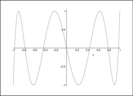
Figure 1: Graph of the polynomial $T_{7}(x).$

We recall that a monic polynomial is a polynomial whose leading coefficient

is $1$.

Property 3 (Monic polynomials of smallest norm)

Let $a,\,b\in\mathbb{R}$, $a\leq b$. The monic degree-$n$ polynomial having the smallest $||.||_{\infty,[a,b]}$ norm in $[a,b]$ is

$$\frac{(b-a)^{n}}{2^{2n-1}}T_{n}\left(\frac{2x-b-a}{b-a}\right).$$

The central result in polynomial approximation theory is the following theorem, due to Chebyshev.

Theorem 1 (Chebyshev)

Let $a,\,b\in\mathbb{R}$, $a\leq b$. The polynomial $p$ is the minimax approximation of degree $\leq n$ to a continuous function $f$ on $[a,b]$ if and only if there exist at least $n+2$ values

$$a\leq x_{0}<x_{1}<x_{2}<\ldots{}<x_{n+1}\leq b$$

such that:

$$p(x_{i})-f(x_{i})=(-1)^{i}\left[p(x_{0})-f(x_{0})\right]=\pm||f-p||_{{\infty,[a,b]}}.$$

Throughout the paper, we will make frequent use of the polynomials

$$T_{n}^{*}(x)=T_{n}(2x-1).$$

The first polynomials $T_{n}^{*}$ are given below. We have (see [4, Chap. 3] for example) $T_{n}^{*}(x)=T_{2n}(x^{1/2})$, hence all the coefficients of $T_{n}^{*}$ are nonzero integers.

$$\begin{array}[]{lll}T_{0}^{*}(x)&=&1,\\ T_{1}^{*}(x)&=&2x-1,\\ T_{2}^{*}(x)&=&8x^{2}-8x+1,\\ T_{3}^{*}(x)&=&32x^{3}-48x^{2}+18x-1,\\ T_{4}^{*}(x)&=&128x^{4}-256x^{3}+160x^{2}-32x+1,\\ T_{5}^{*}(x)&=&512x^{5}-1280x^{4}+1120x^{3}-400x^{2}+50x-1.\\ \end{array}$$

Theorem 2 (Polynomial of smallest norm with degree-$k$ coefficient equal to $1$.)

Let $a\in(0,+\infty)$, define

$$\beta_{0}+\beta_{1}x+\beta_{2}x^{2}+\cdots{}+\beta_{n}x^{n}=T_{n}^{*}\left(\frac{x}{a}\right).$$

Let $k$ be an integer, $0\leq k\leq n$, the polynomial

$$\frac{1}{\beta_{k}}T_{n}^{*}\left(\frac{x}{a}\right).$$

has the smallest $||.||_{\infty,[0,a]}$ norm in $[0,a]$ among the polynomials of degree at most $n$ with a degree-$k$ coefficient equal to $1$. That norm is $|1/\beta_{k}|$.

Moreover, when $k=n=0$ or $1\leq k\leq n$, this polynomial is the only one having this property.

Proving this theorem first requires the following results.

Proposition 1

Let $(\delta_{i})_{i=0,\ldots,n}$ be an increasing sequence of nonnegative integers and

$$P(x)=a_{0}x^{\delta_{0}}+\cdots+a_{n}x^{\delta_{n}}\in\mathbb{R}[x],$$

then either $P=0$ or $P$ has at most $n$ zeros in $(0,+\infty)$.

Proof. By induction on $n$. For $n=0$, it is straightforward. Now we assume that the property is true until the rank $n$. Let $P(x)=a_{0}x^{\delta_{0}}+\cdots+a_{n}x^{\delta_{n}}+a_{n+1}x^{\delta_{n+1}}\in\mathbb{R}[x]$ with $0\leq\delta_{0}<\cdots<\delta_{n+1}$ and $a_{0}a_{1}\ldots a_{n+1}\neq 0$. Assume that $P$ has at least $n+2$ zeros in $(0,+\infty)$. Then $P_{1}=P/x^{\delta_{0}}$ has at least $n+2$ zeros in $(0,+\infty)$.

Thus, the nonzero polynomial $P_{1}^{\prime}(x)=(\delta_{1}-\delta_{0})a_{1}x^{\delta_{1}-\delta_{0}}+\cdots+(\delta_{n+1}-\delta_{0})a_{n+1}x^{\delta_{n+1}-\delta_{0}}$ has, from Rolle’s Theorem, at least $n+1$ zeros in $(0,+\infty)$, which contradicts the induction hypothesis. $\Box$

Corollary 1

Let $k$ be an integer, $1\leq k\leq n$, and

$$P(x)=\displaystyle\sum_{j=0\atop j\neq k}^{n}e_{j}x^{j}\in\mathbb{R}[x].$$

If $P$ has at least $n$ zeros in $[0,+\infty)$ and at most a simple zero in $0$, then $P=0$.

Proof. If $P(0)\neq 0$, then $P$ has at least $n$ zeros in $(0,+\infty)$, hence $P=0$ from Proposition 1. Suppose now that $P(0)=0$. We can rewrite $P$ as $P(x)=\displaystyle\sum_{j=1\atop j\neq k}^{n}e_{j}x^{j}$. As $P$ has at least $n-1$ zeros in $(0,+\infty)$, it must yet vanish identically from Proposition 1. $\Box$

Proof of Theorem 2. We give the proof in the case $a=1$ (the general case is a straightforward generalization).

The case $k=n=0$ is straightforward.

Denote $T_{n}^{*}(x)=\displaystyle\sum_{k=0}^{n}a_{k}x^{k}$. From Property 2, there exist $0=\eta_{0}<\eta_{1}<\cdots<\eta_{n}=1$ such that

$$a_{k}^{-1}T_{n}^{*}(\eta_{i})=a_{k}^{-1}(-1)^{n-i}\left\|T_{n}^{*}\right\|_{\infty,[0,1]}=a_{k}^{-1}(-1)^{n-i}.$$

Now, we assume $1\leq k\leq n$. This part of the proof follows step by step the proof of Theorem 2.1 in [14]. Let $q(x)=\displaystyle\sum_{j=0,\atop j\neq k}^{n}c_{j}x^{j}\in\mathbb{R}[x]$ satisfy $\|x^{k}-q(x)\|_{\infty,[0,1]}\leq|a_{k}^{-1}|$. We suppose that $x^{k}-q\neq a_{k}^{-1}T_{n}^{*}$. Then the polynomial $P(x)=a_{k}^{-1}T_{n}^{*}(x)-(x^{k}-q(x))$ has the form $\displaystyle\sum_{j=0,\atop j\neq k}^{n}d_{j}x^{j}$ and is not identically zero.

Hence there exist $i$ and $j$, $0\leq i<j\leq n$, such that $P(\eta_{0})=\cdots=P(\eta_{i-1})=0$, $P(\eta_{i})\neq 0$ and $P(\eta_{j})\neq 0$, $P(\eta_{j+1})=\cdots=P(\eta_{n})=0$ (otherwise, the nonzero polynomial $P$ would have at least $n$ distinct roots in $[0,1]$ which would contradict Corollary 1). Let $l$ such that $P(\eta_{l})\neq 0$ then sgn $P(\eta_{l})=$ sgn $a_{k}^{-1}T_{n}^{*}(\eta_{l})=(-1)^{n-l}$ sgn $a_{k}^{-1}$. Let $m$ such that $P(\eta_{l})\neq 0$, $P(\eta_{l+1})=\cdots=P(\eta_{l+m-1})=0$, $P(\eta_{l+m})\neq 0$ : $P$ has at least $m-1$ zeros in $[\eta_{l},\eta_{l+m}]$. We distinguish two cases:

• If $m$ is even, we have sgn $P(\eta_{l})=$ sgn $P(\eta_{l+m})$ and thus, $P$ must have an even number of zeros (counted with multiplicity) in $[\eta_{l},\eta_{l+m}]$.

• If $m$ is odd, we have sgn $P(\eta_{l})=-$ sgn $P(\eta_{l+m})$ and thus, $P$ must have an odd number of zeros (counted with multiplicity) in $[\eta_{l},\eta_{l+m}]$.

In both cases, we conclude that $P$ has at least $m$ zeros in $[\eta_{l},\eta_{l+m}]$.

Then $P$ has at least $j-i$ zeros in $[\eta_{i},\eta_{j}]$. Finally, $P$ has not less than $i+(j-i)+n-j=n$ zeros in $[0,1]$ ($P$ has at least $i$ zeros in $[\eta_{0},\eta_{i})$ and at least $n-j$ zeros in $(\eta_{j},\eta_{n}]$). Note that we also obtained that $P$ has no less than $n-1$ zeros in $(0,1]$. As $P$ is nonzero, this contradicts Corollary 1.

To end, we assume $k=0$ and $n\geq 1$. Let $q(x)=\displaystyle\sum_{j=1}^{n}c_{j}x^{j}\in\mathbb{R}[x]$ satisfy $\|1-q(x)\|_{\infty,[0,1]}<|a_{0}^{-1}|$. Then the polynomial $P(x)=a_{0}^{-1}T_{n}^{*}(x)-(1-q(x))$ has the form $\displaystyle\sum_{j=1}^{n}d_{j}x^{j}$ and is not identically zero. This polynomial changes sign between any two consecutive extrema of $T_{n}^{*}$, hence it has at least $n$ zeros in $(0,1)$. As it cancels also at $0$, we deduce that $P$ vanishes identically, which is the contradiction desired. $\Box$

Remark 1

When $k=0$ and $n\geq 1$, it is not possible to prove unicity: for example, let $a=1$, $k=0$, $n=1$, the polynomials $1-\lambda x$ with $\lambda\in[0,2]$ have all a $||.||_{\infty,[0,1]}$ norm equal to $1$.

2 Getting the “truncated” polynomial that is closest to a function in $[0,a]$

Let $a\in(0,+\infty)$, let $f$ be a function defined on $[0,a]$ and $m_{0}$, $m_{1}$, …, $m_{n}$ be $n+1$ integers. Define ${\cal P}_{n}^{[m_{0},m_{1},\ldots{},m_{n}]}$ as the set of the polynomials of degree less than or equal to $n$ whose degree-$i$ coefficient is a multiple of $2^{-m_{i}}$ for all $i$ between $0$ and $n$ (we will call these polynomials “truncated polynomials”).

Let $p$ be the minimax approximation to $f$ on $[0,a]$. Define $\hat{p}$ as the polynomial whose degree-$i$ coefficient is obtained by rounding the degree-$i$ coefficient of $p$ to the nearest multiple of $2^{-m_{i}}$ (with an arbitrary choice in case of a tie) for $i=0,\ldots,\,n$: $\hat{p}$ is an element of ${\cal P}_{n}^{[m_{0},m_{1},\ldots{},m_{n}]}$.

Also define ${\epsilon}$ and $\hat{\epsilon}$ as

$$\epsilon=||f-p||_{\infty,[0,a]}\,\mbox{ and }\,\hat{\epsilon}=||f-\hat{p}||_{\infty,[0,a]}.$$

We assume that $\hat{\epsilon}\neq 0$. Let $\lambda\in\left[\frac{\epsilon}{\hat{\epsilon}},1\right]$, we are looking for a truncated polynomial $p^{\star}\in{\cal P}_{n}^{[m_{0},m_{1},\ldots{},m_{n}]}$ such that

$$||f-p^{\star}||_{\infty,[0,a]}=\min_{q\in{\cal P}_{n}^{[m_{0},m_{1},\ldots{},m_{n}]}}||f-q||_{\infty,[0,a]}$$

and

$$||f-p^{\star}||_{\infty,[0,a]}\leq\lambda||f-\hat{p}||_{\infty,[0,a]}.$$ (3)

When $\lambda=1$, this problem has a solution since $\hat{p}$ satisfies (3). It should be noticed that, in that case, $p^{\star}$ is not necessarily equal to $\hat{p}$.

In the following, we compute bounds on the coefficients of a polynomial $q\in{\cal P}_{n}^{[m_{0},m_{1},\ldots{},m_{n}]}$ such that if $q$ is not within these bounds, then

$$||p-q||_{\infty,[0,a]}>\epsilon+\lambda\hat{\epsilon}.$$

Knowing these bounds will allow an exhaustive searching of $p^{\star}$. To do that, consider a polynomial $q$ whose degree-$i$ coefficient is $p_{i}+\delta_{i}$, with $\delta_{i}\neq 0$. Let us see how close can $q$ be to $p$. We have

$$(q-p)(x)=\delta_{i}x^{i}+\sum_{0\leq j\leq n,\atop j\neq i}(q_{j}-p_{j})x^{j}.$$

Hence, $||q-p||_{\infty,[0,a]}$ is minimum implies that

$$||x^{i}+\frac{1}{\delta_{i}}\sum_{0\leq j\leq n,\atop j\neq i}(q_{j}-p_{j})x^{j}||_{\infty,[0,a]}$$

is minimum.

Hence, we have to find the polynomial of degree $n$, with fixed degree-$i$ coefficient, whose norm is smallest. This is given by Theorem 2. Therefore, we have

$$||x^{i}+\frac{1}{\delta_{i}}\sum_{0\leq j\leq n,\atop j\neq i}(q_{j}-p_{j})x^{j}||_{\infty,[0,a]}\geq\frac{1}{|\beta_{i}|},$$

where $\beta_{i}$ is the nonzero degree-$i$ coefficient of $T_{n}^{*}(x/a)$. Therefore, we must have

$$||q-p||_{\infty,[0,a]}\geq\frac{\delta_{i}}{|\beta_{i}|}.$$

Now, if a polynomial is at a distance greater than $\epsilon+\lambda\hat{\epsilon}$ from $p$, it cannot be $p^{\star}$ since

$$||q-f||_{\infty,[0,a]}\geq||q-p||_{\infty,[0,a]}-||p-f||_{\infty,[0,a]}>\lambda\hat{\epsilon}.$$

Therefore, if there exists $i$, $0\leq i\leq n$, such that

$$|\delta_{i}|>(\epsilon+\lambda\hat{\epsilon})|\beta_{i}|$$

then $||q-p||>\epsilon+\lambda\hat{\epsilon}$ and therefore $q\neq p^{\star}$. Hence, the degree-$i$ coefficient of $p^{\star}$ necessarily lies in the interval $[p_{i}-(\epsilon+\lambda\hat{\epsilon})|\beta_{i}|,p_{i}+(\epsilon+\lambda\hat{\epsilon})|\beta_{i}|]$. Thus we have

$$\underbrace{\left\lceil 2^{m_{i}}(p_{i}-(\epsilon+\lambda\hat{\epsilon})|\beta_{i}|)\right\rceil}_{m_{i}}\leq 2^{m_{i}}{p_{i}^{\star}}\leq\underbrace{\left\lfloor 2^{m_{i}}(p_{i}+(\epsilon+\lambda\hat{\epsilon})|\beta_{i}|)\right\rfloor}_{M_{i}},$$ (4)

since $2^{m_{i}}{p_{i}^{\star}}$ is a rational integer: we have $M_{i}-m_{i}+1$ possible values for the integer $2^{m_{i}}{p_{i}^{\star}}$. This means that we have $\prod_{i=0}^{n}(M_{i}-m_{i}+1)$ polynomials candidates. If this amount is small enough, we search for $p^{\star}$ by computing the norms $||f-q||_{\infty,[0,a]}$, $q$ running among the possible polynomials. Otherwise, we need an additional step to decrease the number of candidates. Hence, we give now a method for this purpose.

Condition (3) means

$$f(x)-\lambda\hat{\epsilon}\leq\sum_{i=0}^{n}{p_{i}^{\star}}x^{i}\leq f(x)+\lambda\hat{\epsilon}$$ (5)

for all $x\in[0,a]$. In particular, we have

$$f(0)-\lambda\hat{\epsilon}\leq p_{0}^{\star}\leq f(0)+\lambda\hat{\epsilon}$$

i.e., since $2^{m_{0}}p_{0}^{\star}$ is an integer,

$$\lceil 2^{m_{0}}(f(0)-\lambda\hat{\epsilon})\rceil\leq 2^{m_{0}}p_{0}^{\star}\leq\lfloor 2^{m_{0}}(f(0)+\lambda\hat{\epsilon})\rfloor.$$

The $n+1$ inequations given by (4) define a polytope to which the numerators (i.e. the $2^{m_{i}}p_{i}^{\star}$) belong. The idea is to try to make this polytope smaller in order to reduce our final exhaustive search. We do that thanks to inequations (5) considered for a certain number (chosen by the user) of values of $x\in[0,a]$. Once we got a small enough polytope, we start our exhaustive search using libraries (such as Polylib [11] and CLooG [2]) specially designed for scanning efficiently the integer points of polytopes and producing only the corresponding loops in our program of exhaustive search. CLooG implements the Quilleré et al. algorithm [12].

3 Examples

We implemented in Maple a weakened version of the process described in the previous section. By this, we mean that in the step of refinement of the polytope, we only determine its vertices using the simplex method instead of scanning its integer points. The program first computes the bounds obtained from Chebyshev polynomials and then, if these bounds are too large, computes the vertices of the polytope obtained from inequations (4) and inequations (5) considered for $x_{i}=\frac{i}{d}A$ where $d$ is an integer parameter chosen by the user, $i$ an integer, $0\leq i\leq d$ and $A$ is a rational number “close” and less than or equal to $a$.

3.1 Cosine function in $[0,\pi/4]$ with a degree-$3$ polynomial

In $[0,\pi/4]$, the distance between the cosine function and its best degree-$3$ minimax approximation is $0.00011$. This means that such an approximation is not good enough for single-precision implementation of the cosine function. It can be of interest for some special-purpose implementations. In this example, the bounds given by the first step (associated to Chebyshev polynomials) are good enough to avoid the use of the polytope refinement.

>m := [12,10,6,4]:polstar(cos,Pi/4,3,m);

  "minimax = ", .9998864206

         + (.00469021603 + (-.5303088665 + .06304636099 x) x) x

            "Distance between f and p =", .0001135879209

                            3   17  2     5
              "hatp = ", - x  - -- x  + ---- x + 1
                                32      1024


           "Distance between f and hatp =", .0006939707


>Do you want to continue (y;/n;)? y;
>Enter the value of parameter lambda: 1/2;

degree 0: 4 possible values between 2047/2048 and
          4097/4096
degree 1: 22 possible values between -3/512 and
          15/1024
degree 2: 5 possible values between -9/16 and
          -1/2
degree 3: 1 possible values between 1/16 and
          1/16
440 polynomials need be checked

>Do you want to try to refine the bounds (y;/n;)?n;


                            1  3   17  2    3      4095
             "pstar = ",   -- x  - -- x  + --- x + ----
                           16      32      512     4096


           "Distance between f and pstar =", .0002441406250

                "Time elapsed (in seconds) =", 1.840

In this example, the distance between $f$ and $p^{*}$ is approximately $0.35$ times the distance between $f$ and $\hat{p}$. Using our method saves around $-\log_{2}(0.35)\approx 1.5$ bits of accuracy.

3.2 Exponential function in $[0,\log(1+1/2048)]$ with a degree-$3$ polynomial

In $[0,\log(1+1/2048)]$, the distance between the exponential function and its best degree-$3$ minimax approximation is around $1.8\times 10^{-17}$, which should be sufficient for a faithfully rounded double precision implementation provided there is much care in the polynomial evaluation. The bounds given to get $p^{\star}$ using the first step are too large (there are 18523896 polynomials to test). Hence, we must use the polytope refinement.

>Digits:=30:
>m := [56,45,33,23]: polstar(exp,log(1.+1./2048),3,m);

"minimax = ", .999999999999999981509827946165 +
(1.00000000000121203815619648271
 + (.499999987586063030320493910112
 + .166707352549861488779274879363 x) x) x

                                                   -16
    "Distance between f and p =", .1849017208895 10


             1398443  3   4294967189  2   35184372088875
  "hatp = ", ------- x  + ---------- x  + -------------- x
             8388608      8589934592      35184372088832


           72057594037927935
         + -----------------
           72057594037927936


    "Distance between f and hatp =",
                                            -16
                 .23624220969326235229443 10

>Do you want to continue (y;/n;)? y;
>Enter the value of parameter lambda: 1;

degree 0: 6 possible values between
18014398509481983/18014398509481984
          and 72057594037927937/72057594037927936
degree 1: 109 possible values between
35184372088821/35184372088832
          and 35184372088929/35184372088832
degree 2: 146 possible values between 4294967117/8589934592
          and 2147483631/4294967296
degree 3: 194 possible values between 699173/4194304
          and 1398539/8388608
18523896 polynomials need be checked

>Do you want to try to refine the bounds (y;/n;)?y;
>Enter the value of parameter d: 25;

degree 0: 2 possible values between
72057594037927935/72057594037927936
          and 1
degree 1: 27 possible values between 35184372088857/35184372088832
          and 35184372088883/35184372088832
degree 2: 32 possible values between 536870897/1073741824
          and 4294967207/8589934592
degree 3: 44 possible values between 1398421/8388608
          and 21851/131072
76032 polynomials need be checked


>Do you want to try to refine the bounds (y;/n;)?n;
>Do you want to change the value of Digits (y;/n;)?y;
>Enter the value of Digits: 21;

            1398443  3   2147483595  2   35184372088873
"pstar = ", ------- x  + ---------- x  + -------------- x
            8388608      4294967296      35184372088832

           72057594037927935
         + -----------------
           72057594037927936

    "Distance between f and pstar =",
                                            -16
                 .20246280367096470182285 10

         "Time elapsed (in seconds) =", 54721.961

In this last example, the distance between $f$ and $p^{*}$ is approximately $0.85$ times the distance between $f$ and $\hat{p}$. Using our method saves around $-\log_{2}(0.85)\approx 0.22$ bits of accuracy.

References

- [1] P. Borwein and T. Erdélyi, Polynomials and Polynomials Inequalities, Graduate Texts in Mathematics, 161, Springer-Verlag, 1995.
- [2] C. Bastoul. CLooG, a loop generator for scanning Z-polyhedra, User’s Guide, available from http://www.prism.uvsq.fr/~cedb/bastools/cloog.html.
- [3] M. Daumas, C. Mazenc, X. Merrheim, and J.- M. Muller. Modular range reduction: A new algorithm for fast and accurate computation of the elementary functions. Journal of Universal Computer Science, 1(3):162–175, March 1995.
- [4] L. Fox and I. B. Parker, Chebyshev Polynomials in Numerical Analysis, Oxford Mathematical Handbooks, Oxford University Press, 1972.
- [5] J. F. Hart, E. W. Cheney, C. L. Lawson, H. J. Maehly, C. K. Mesztenyi, J. R. Rice, H. G. Thacher, and C. Witzgall. Computer Approximations. Wiley, New York, 1968.
- [6] P. Markstein. IA-64 and Elementary Functions: Speed and Precision. Hewlett-Packard Professional Books. Prentice Hall, 2000. ISBN: 0130183482.
- [7] J.-M. Muller. Elementary Functions, Algorithms and Implementation. Birkhäuser, Boston, 1997.
- [8] K. C. Ng. Argument reduction for huge arguments: Good to the last bit (can be obtained by sending an e-mail to the author: kwok.ng@eng.sun.com). Technical report, SunPro, 1992.
- [9] M. Payne and R. Hanek. Radian reduction for trigonometric functions. SIGNUM Newsletter, 18:19–24, 1983.
- [10] J.A. Pineiro, J.D. Bruguera, and J.-M. Muller. Faithful powering computation using table look-up and a fused accumulation tree. In Burgess and Ciminiera, editors, Proc. of the 15th IEEE Symposium on Computer Arithmetic (Arith-15). IEEE Computer Society Press, 2001.
- [11] Polylib, a library of polyhedral functions, User’s Manual, available from http://www.irisa.fr/polylib/.
- [12] F. Quilleré, S. Rajopadhye and D. Wilde. Generation of efficient nested loops from polyhedra. International Journal of Parallel Programming, 28(5):469–498, October 2000.
- [13] E. Remes. Sur un procédé convergent d’approximations successives pour déterminer les polynômes d’approximation. C.R. Acad. Sci. Paris, 198, 1934, pp 2063–2065.
- [14] T. J. Rivlin. Chebyshev polynomials. From approximation theory to algebra and number theory. Second edition. Pure and Applied Mathematics. John Wiley & Sons, Inc., New York, 1990.
- [15] P. T. P. Tang. Table-driven implementation of the exponential function in IEEE floating-point arithmetic. ACM Transactions on Mathematical Software, 15(2):144–157, June 1989.
- [16] P. T. P. Tang. Table-driven implementation of the logarithm function in IEEE floating-point arithmetic. ACM Transactions on Mathematical Software, 16(4):378–400, December 1990.
- [17] P. T. P. Tang. Table lookup algorithms for elementary functions and their error analysis. In P. Kornerup and D. W. Matula, editors, Proceedings of the 10th IEEE Symposium on Computer Arithmetic, pages 232–236, Grenoble, France, June 1991. IEEE Computer Society Press, Los Alamitos, CA.
- [18] P. T. P. Tang. Table-driven implementation of the expm1 function in IEEE floating-point arithmetic. ACM Transactions on Mathematical Software, 18(2):211–222, June 1992.
- [19] B. Wei, J. Cao and J. Cheng. High-performance architectures for elementary function generation. In Burgess and Ciminiera, editors, Proc. of the 15th IEEE Symposium on Computer Arithmetic (Arith-15). IEEE Computer Society Press, 2001.