State Complexes for Metamorphic Robots

Abstract

A metamorphic robotic system is an aggregate of homogeneous robot units which can individually and selectively locomote in such a way as to change the global shape of the system. We introduce a mathematical framework for defining and analyzing general metamorphic robots. This formal structure, combined with ideas from geometric group theory, leads to a natural extension of a configuration space for metamorphic robots — the state complex — which is especially adapted to parallelization. We present an algorithm for optimizing reconfiguration sequences with respect to elapsed time. A universal geometric property of state complexes — non-positive curvature — is the key to proving convergence to the globally time-optimal solution.

1 Introduction

In recent years, several groups in the robotics community have been modeling and building reconfigurable or, more specifically, metamorphic robots (e.g., [8, 14, 16, 23, 24]). Such a system consists of multiple identical robotic cells in an underlying lattice structure which can disconnect/reconnect with adjacent neighbors, and slide, pivot, or otherwise locomote to neighboring lattice points following prescribed rules: see Fig. 1. There are as many models for such robots as there are researchers in the sub-field: 2-d and 3-d lattices; hexagonal, square, and dodecahedral cells; pivoting or sliding motion: see, e.g., [8, 14, 15, 16, 17, 7, 18, 23, 24] and the references therein. The common feature of these robots is an aggregate of lattice-based cells having prescribed local transitions from one shape to another.

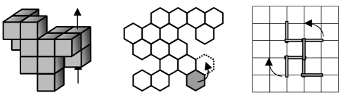
Fig. 1: Metamorphic systems may be built on a variety of lattice structures with sliding or pivoting motion.

The primary challenge for such systems is shape-planning: how to move from one shape to another via legal moves. One centralized approach [9, 20] is to build a transition graph whose vertices are the various shapes and whose edges are elementary legal moves from one shape to the next. It is easily demonstrated that the size of this graph is exponential in the number of cells.

We propose to extend the notion of a configuration space to metamorphic robots in a novel manner. The idea: consider the transition graph described above as a one-dimensional skeleton of a higher-dimensional cubical complex, the state complex. Assume that from a given state there are two legal moves which are physically independent (or, more suggestively, “commutative”): i.e., these moves can be executed simultaneously. In the transition graph, this corresponds to the four edges of a square. For any pair of commutative moves, fill in the four edges of the graph with an abstract square 2-cell. Continue inductively adding $k$-dimensional cubes corresponding to $k$-tuples of physically independent motions. The result is a cubical complex which has several advantages over the transition graph:

1. Simplicity. The state complex is often simpler than the transition graph: e.g., the 1-d graph of an $n$-dimensional cube has $n2^{n-1}$ edges. This figure belies the simplicity of the single cube.

2. Speed. Geodesics on this complex cut across the diagonals of cubes whenever possible. One performs all possible commutative motions simultaneously, maximizing parallelization and yielding a speed-up by a factor equal to the number of coordinated motions.

3. Shape. The global geometry/topology of the state complex carries information about the metamorphic system. For certain examples, the topology of the state complex “converges” upon refining the lattice. In addition, only special geometries can be realized as the state complex of a local metamorphic system: commutativity in reconfiguration leads to an abhorrence of positive curvature in the state complex.

Sections 2 through 4 give definitions and examples of [abstract] metamorphic systems and their state complexes. The next two sections (Sections 5-6) detail topological and geometric features of the state complex.

For large systems, the problem of computing the state complex and designing geodesics in order to perform shape planning is computationally infeasible, primarily because the size of the complex is often exponential in the number of robot cells. In addition, any control scheme induced by geodesic construction is necessarily centralized. Several researchers have begun building decentralized control algorithms for shape planning [6, 22, 21, 25, 26]. Such algorithms have the advantage of speed and scalability; however, the reconfiguration paths are typically not optimal.

As an application of our techniques, we present in Sections 7-8 an algorithm for trajectory optimization which takes as its argument an arbitrary edge path in the transition graph. Algorithm 28 then performs a type of curve shortening within the state complex. A deep theorem about the curvature of all state complexes (Theorem 20) is then used to prove that this algorithm returns a shape trajectory which is the global minimum obtainable from this path with respect to elapsed time.

Our definitions and theorems are phrased for systems involving “discrete” reconfiguration. More general types of robots which employ continuous reconfiguration for locomotive gaits (such as the Polybot developed by M. Yim’s lab at Xerox PARC) are not covered by our definitions. We note, however, that certain locomotive reconfigurable robots can be thought of as lattice-based tiles by amalgamating subsystems [15]. In addition, our definitions can easily be extended to more general non-lattice reconfigurable systems [4].

2 A mathematical definition

While it is easy to generate examples of what is meant by a metamorphic robot, it is more challenging to write a clean mathematical definition. We propose a set of definitions which is broad enough to include some non-obvious examples. The paper [7] suggests a similar type of structure using cellular automata rule sets.

A local metamorphic system is a collection of states on a lattice, where each state is thought of as an indicator function for the aggregate. Any state can be modified by local rearrangements, these local changes being coordinated by a catalogue of models realized under the actions of isometries into the workspace. The adjective “local” refers to legality criteria: anywhere in the workspace at which a local change from the catalogue can be applied, it is legal to do so. To incorporate obstacles and basepoints into our systems, we distinguish between the amount of information needed to determine the legality of an elementary move (the “support” of the move) and the precise place in which modules are actually in motion (the “trace” of the move).

Definition 1.

Let ${\mathcal{L}}$ denote a lattice in $\mathbb{R}^{k}$ and let ${\mathcal{W}}\subset{\mathcal{L}}$ be some workspace. The catalogue ${\sf C}$ for a local metamorphic system on ${\mathcal{W}}$ is a collection of generators. Each generator ${\mathbf{\phi}}\in{\sf C}$ consists of (1) the support, ${\mbox{\sc sup}}({\mathbf{\phi}})\subset{\mathcal{L}}$; (2) the trace of the move, ${\mbox{\sc tr}}({\mathbf{\phi}})\subset{\mbox{\sc sup}}({\mathbf{\phi}})$; and (3) an unordered pair of local states ${\hat{U}}_{0,1}:{\mbox{\sc sup}}({\mathbf{\phi}})\to\{0,1\}$ satisfying

$${\left.{{\hat{U}}_{0}}\right|_{{\mbox{\sc sup}}({\mathbf{\phi}})-{\mbox{\sc tr}}({\mathbf{\phi}})}}={\left.{{\hat{U}}_{1}}\right|_{{\mbox{\sc sup}}({\mathbf{\phi}})-{\mbox{\sc tr}}({\mathbf{\phi}})}}.$$ (1)

Otherwise said, the local states are equal on ${\mbox{\sc sup}}({\mathbf{\phi}})-{\mbox{\sc tr}}({\mathbf{\phi}})$.

Definition 2.

An action of a generator ${\mathbf{\phi}}\in{\sf C}$ is a rigid translation ${\mathbf{\Phi}}:{\mbox{\sc sup}}({\mathbf{\phi}})\hookrightarrow{\mathcal{W}}$. Given a state ${U}:{\mathcal{W}}\to\{0,1\}$, an action ${\mathbf{\Phi}}$ is said to be admissible at ${U}$ if ${\hat{U}}_{0}={U}\circ{\mathbf{\Phi}}$. In this case, we write

$${\mathbf{\phi}}[{U}]:=\left\{\begin{array}[]{cl}{U}&:{\mbox{ on }}{\mathcal{W}}-{\mathbf{\Phi}}({\mbox{\sc sup}}({\mathbf{\phi}}))\\ {\hat{U}}_{1}\circ{\mathbf{\Phi}}{{}^{-1}}&:{\mbox{ on }}{\mathbf{\Phi}}({\mbox{\sc sup}}({\mathbf{\phi}}))\end{array}\right..$$

(Note that ${\mathbf{\Phi}}$ is left out of the notation.)

Definition 3.

A local metamorphic system on ${\mathcal{W}}$ is a collection of finite states $\{{U}_{\alpha}:{\mathcal{W}}\to\{0,1\}\}$ closed under all possible admissible actions of generators in the catalogue ${\sf C}$. (A state is finite if ${U}=1$ at only finitely many points of ${\mathcal{W}}$.)

To repeat, the catalogue and the workspace are the “seeds” for a local metamorphic system. From this pair, all possible translations of the supports into ${\mathcal{W}}$ yield the actions. Then, a collection of states on the workspace is a local metamorphic system if, whenever an action ${\mathbf{\Phi}}$ of a generator ${\mathbf{\phi}}$ on a state ${U}$ is admissible, then the corresponding state ${\mathbf{\phi}}[{U}]$ is also included.

A metamorphic system with obstacles ${\mathcal{O}}\subset{\mathcal{W}}$ satisfies in addition

$${\mathbf{\Phi}}({\mbox{\sc tr}}({\mathbf{\phi}}))\cap{\mathcal{O}}=\emptyset,$$ (2)

for each ${\mathbf{\phi}}\in{\sf C}$. Obstacle sets count as legal positions for determining the admissibility of a move (the support of an action may intersect ${\mathcal{O}}$), but no motion of metamorphic agents may incorporate the obstacle sites (the trace of an action must not intersect ${\mathcal{O}}$).

3 Examples

Some of the following examples are inspired by metamorphic robots already developed; other examples are more abstract.

Example 4.

[2-d hex with pivots] We present two slightly different catalogues, each with six generators (or one, up to discrete rotations), in Fig. 2. Both of these systems, modeled after that of [8], have local moves which pivot a planar hexagon about a neighbor. For all generators presented, the trace is equal to the two central hexagons. In the first system, the support is chosen so that the aggregate does not change its topology but only its shape. The slightly smaller support of the second catalogue allows for local topology changes. To model a fixed “base” cell (which is, say, affixed to a power source as in [18]), one establishes this cell as an obstacle ${\mathcal{O}}$.

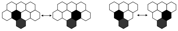
Fig. 2: Two different catalogues for a 2-d hexagonal lattice system with pivots. Black cells are occupied, white are unoccupied. The local states ${\hat{U}}_{0}$ and ${\hat{U}}_{1}$ are shown for each generator.

Example 5.

[2-d square lattice] In Fig. 3, we display a generator for a planar system in which rows [as pictured] and columns [not pictured] of an aggregate of square cells can slide. There are in fact several generators represented in “shorthand,” one for each $k\geq 0$. A dot inside a cell indicates that it can be either occupied or unoccupied, but if occupied, then its neighbor (indicated by an arrow) must also be turned on. This condition guarantees that the aggregate does not disconnect (even locally) under slides. The trace of this set of generators is the entire middle row except the two endpoints. To keep the catalogue finite, one would include only those generators with $k\leq N$, where $N$ is the number of occupied cells in any state.

\psfragscanon\psfrag{k}[bc][bc]{\Large{$k$}}\psfrag{0}[c][c]{\Large{$0$}}\psfrag{1}[c][c]{\Large{$1$}}\includegraphics[angle={0},width=354.12256pt]{squareex2.ps}

Fig. 3: The row-sliding generators for a sliding-squares system.

Example 6.

[2-d articulated planar arm] Consider as a workspace ${\mathcal{W}}$ the set of edges in the planar integer lattice. The catalogue consists of two generators, pictured in Fig. 4. Beginning with a state having $N$ vertical edges end-to-end, the metamorphic system thus generated models the position of an articulated robotic arm with fixed base which can (1) rotate at the top end and (2) flip corners as per the diagram.

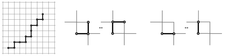
Fig. 4: A positive articulated robot arm [left]. One generator [center] flips corners and has as its trace the central four edges. The other generator [right] rotates the end of the arm, and has trace equal to the two activated edges.

If one includes rotations of these generators, more intricate types of configurations are possible, including deadlocked configurations. Highly self-reconfigurable examples with multiple interacting arms can be realized by adding new generators: an “attach-detach” generator which allows endpoints of arms to merge (thus yielding a “marked point” at the attachment); and a “sliding” generator which allows this marked point to slide, having the effect of allowing the attached arms to trade segments. These generators are pictured (up to Euclidean symmetries) in Figure 5.

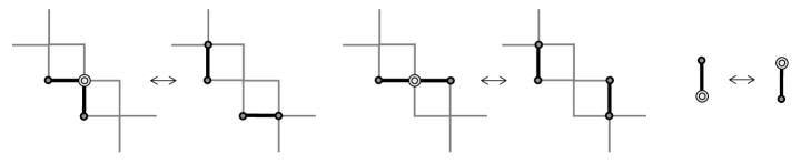
Fig. 5: Additional generators allow for attachment and detachment of arm endpoints [left, center] and sliding of the coupling points [right].

One of the benefits of writing down a rigorous definition of a metamorphic system is the discovery of systems which have little resemblance to the systems of, say, Fig. 1. In particular, our definitions easily extend to metamorphic systems which are not lattice-based; the following example is especially interesting.

Example 7.

Consider a finite graph $\Gamma$ in which every edge is assigned a length of one. (Every graph can be embedded in some $\mathbb{R}^{k}$ so as to have this property.) The catalogue consists of a single generator whose support and trace are precisely the closure of a single “abstract edge.” The local states of this generator consist of the pair ${\hat{U}}_{0}$ and ${\hat{U}}_{1}$ which evaluate to $1$ on one of the endpoints and $0$ on the other. The actions in this case are length-preserving maps from the abstract edge into $\Gamma$. The metamorphic system generated from a state ${U}$ on $\Gamma$ with $N$ vertices evaluating to $1$ mimics an ensemble of $N$ unlabeled non-colliding Automated Guided Vehicles on $\Gamma$, cf. [12].

More abstract examples of metamorphic examples include spaces of triangulations of polygons with edge-flipping as the generator, examples arising from word representations in group theory, and certain multi-step assembly processes [4].

4 The state complex

In the robotics literature, one often models a configuration space for a metamorphic system with a transition graph which represents actions of elementary moves on states. That is, the vertex set is the collection of all states $\{{U}_{\alpha}\}$, and the edges are unoriented pairs of states which differ by the action of one generator. Transition graphs are discussed for shape-planning in several particular cases in the literature (planar hex case: [9, 20]). Our departure is to make the transition graph the 1-skeleton of a cubical complex (an analogue of a simplicial complex, but made out of abstract cubes) which coordinates parallel or “commutative” motions.

Definition 8.

In a local metamorphic system, a collection of actions of (not necessarily distinct) generators $\{({\mathbf{\phi}}_{\alpha_{i}},{\mathbf{\Phi}}_{\alpha_{i}})\}$ is said to commute if

$${\mathbf{\Phi}}_{\alpha_{i}}({\mbox{\sc tr}}({\mathbf{\phi}}_{\alpha_{i}}))\cap{\mathbf{\Phi}}_{\alpha_{j}}({\mbox{\sc sup}}({\mathbf{\phi}}_{\alpha_{j}}))=\emptyset\quad\forall i\neq j.$$ (3)

Example 9.

Two simple examples suffice to illustrate the difference between commuting and noncommuting actions. First, consider the pair of commuting moves for a planar hexagonal pivoting system, as represented in Fig. 6 [left].

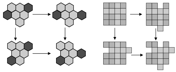
Fig. 6: Examples of commuting [left] and noncommuting [right] actions in planar systems.

Compare this with a planar sliding block example as illustrated in Fig. 6 [right]. Although the pair of moves illustrated forms a square in the transition graph, this particular pair of actions does not commute. Physically, it is obvious why these moves are not independent: sliding the column part-way obstructs sliding a transverse row. Mathematically, this is captured by the traces of the actions intersecting.

The state complex has an abstract $k$-cube for each collection of $k$ admissible commuting actions:

Definition 10.

The state complex ${\mathcal{S}}$ of a local metamorphic system is the following abstract cubical complex. Each abstract $k$-cube $e^{(k)}$ of ${\mathcal{S}}$ is an equivalence class $[{U};({\mathbf{\Phi}}_{\alpha_{i}})_{i=1}^{k}]$ where

1. $({\mathbf{\Phi}}_{\alpha_{i}})_{i=1}^{k}$ is a $k$-tuple of commuting actions of generators $\phi_{\alpha_{i}}$;

2. ${U}$ is some state for which all the actions $({\mathbf{\Phi}}_{\alpha_{i}})_{i=1}^{k}$ are admissible; and

3. $[{U}_{0};({\mathbf{\Phi}}_{\alpha_{i}})_{i=1}^{k}]=[{U}_{1};({\mathbf{\Phi}}_{\beta_{i}})_{i=1}^{k}]$ if and only if the list $(\beta_{i})$ is a permutation of $(\alpha_{i})$ and ${U}_{0}={U}_{1}$ on the set ${\mathcal{W}}-\bigcup_{i}{\mathbf{\Phi}}_{\alpha_{i}}({\mbox{\sc sup}}({\mathbf{\phi}}_{\alpha_{i}}))$ .

The boundary of each abstract $k$-cube is the collection of $2k$ faces obtained by deleting the $i^{th}$ action from the list and using ${U}$ and ${\mathbf{\phi}}_{\alpha_{i}}[{U}]$ as the ambient states. Specifically,

$$\partial[{U};({\mathbf{\Phi}}_{\alpha_{i}})_{i=1}^{k}]=\bigcup_{i=1}^{k}\left([{U};({\mathbf{\Phi}}_{\alpha_{j}})_{j\neq i}]\cup[{\mathbf{\phi}}_{\alpha_{i}}[{U}];({\mathbf{\Phi}}_{\alpha_{j}})_{j\neq i}]\right).$$ (4)

It follows easily that the $k$-cells are well-defined with respect to admissibility of actions. The proof of the following obvious lemma is given in detail to flesh out the previous definition.

Lemma 11.

(a) The 0-dimensional skeleton of ${\mathcal{S}}$, ${\mathcal{S}}^{(0)}$, is the set of states in the reconfigurable system. (b) The 1-dimensional skeleton of ${\mathcal{S}}$, ${\mathcal{S}}^{(1)}$, is precisely the transition graph.

proof:   (a) Vertices of ${\mathcal{S}}$ consist of equivalence classes consisting of zero (i.e., no) actions of generators up to permutation, together with a state defined on the complement of the supports of the actions. As there are no actions, each 0-cell is precisely a single state of the reconfigurable system.

(b) A 1-cell of ${\mathcal{S}}$ is an equivalence class of the form $[{U};({\mathbf{\Phi}})]$. The only other representative of the equivalence class is $[{\mathbf{\phi}}[{U}];({\mathbf{\Phi}})]$; hence, the 1-cells are precisely the edges in the transition graph. Clearly, the boundary of $[{U};({\mathbf{\Phi}})]$ is the pair of 0-cells $[{U};(\cdot)]$ and $[{\mathbf{\phi}}[{U}];(\cdot)]$. ∎

For small numbers of cells, it is easy to illustrate the state complex.

\psfragscanon\psfrag{p}[t]{{\Huge$p$ }}\psfrag{q}[l]{{\Huge$q$ }}\includegraphics[angle={0},width=289.07999pt]{sqshex.ps}

Fig. 7: The planar sliding square example [left] with two movable blocks [in black] and a $p$-by-$q$ obstacle set [in grey] yields a state complex ${\mathcal{S}}$ that is topologically a circle [right].

Example 12.

Consider the 2-d square lattice row/column sliding system whose catalogue is illustrated in Fig. 3. If we consider a system with (occupied) obstacles in the form of a $p$-by-$q$ rectangle generated from the state of Fig. 7 [left], one obtains a planar transition graph with $4(pq+1)+2(p+q)$ vertices and $8(pq+1)-2(p+q)$ edges. In contrast, the state complex is that of Fig. 7 [right]: this is topologically a circle, corresponding to the fact that the pair of free squares can circulate about the obstacle set through a sequence of slides. The large 2-d regions correspond to states in which the two free squares are on separate (but adjacent) sides of the obstacle set.

Example 13.

Consider the planar hex system of Fig. 4 [left] with a workspace ${\mathcal{W}}$ consisting of a long channel of four rows, the bottom row being filled obstacles, and the top row being non-occupied obstacles. A line of cells in one of the two free rows can “climb across” one by one, yielding the state complex of Fig. 8[right] (cf. the algorithm of [21]). This state complex is contractible for any length column.

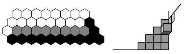
Fig. 8: For a line of hexagons filing out of a constrained tunnel [left], the state complex is contractible [right]. Black cells represent occupied obstacle sets; the top row is an unoccupied obstacle set. A fairly short tunnel is shown: for longer tunnels, the state complex is still contractible, but of higher dimension.

Example 14.

The state complex associated to the positive articulated robot arm of Example 6 in the case $N=5$ is given in Fig. 9. Note that there can be at most three independent motions (when the arm is in a “staircase” configuration); hence the state complex has top dimension three. Notice also that although the transition graph for this system is complicated, the state complex itself is topologically trivial (contractible).

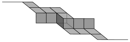
Fig. 9: The state complex of a 5-link positive arm has one cell of dimension three, along with several cells of lower dimension.

Example 15.

In the system of Example 7 with the graph being a $K_{5}$ (the complete graph on five vertices) and $N=2$, the state complex is a two-dimensional closed surface. A simple combinatorial argument (as in [2, 3]) reveals that the Euler characteristic is $-5$, implying that the state complex is non-orientable. If the AGV’s are labeled, the state complex becomes a closed orientable surface of genus 6.

5 The topology of ${\mathcal{S}}$

If one looks at a transition graph without knowing the particulars of the metamorphic system, very little information can be extracted. This paper argues that completing the transition graph to the state complex is “natural” — the state complex simplifies the transition graph and endows it with topological and geometric content.

Our first example of naturality is motivated by the desire to build metamorphic systems with large numbers of micro- or nano-scale cells. While large numbers of cells would yield a type of continuum-limit convergence on the dynamics of shape change, the resulting transition graphs have no such convergence. The size of the transition graph goes up exponentially in the number of cells; more ominous is that the topology of the transition graph (the number of basic cycles) blows up as well. This is not always so with the state complex: in certain key examples, the topology of ${\mathcal{S}}$ is either invariant or converges to a limiting type.

We have already seen one such example of this stabilization. In Example 12, the state complex of a pair of squares sliding along a rectangular obstacle of size $p$-by-$q$ is topologically a circle, independent of $p$ and $q$. This can be interpreted as a type of convergence: consider the effect of refining the underlying lattice structure, increasing $p$ and $q$ while maintaining a pair of sliding squares. Then the dimension of the state complex remains the same, as does the topological type of the space. Intuitively speaking, the “limit” as this refining process is repeated yields a “topological” configuration space of two points sliding smoothly along the boundary of a rectangle, which can dock or un-dock at the corners.

Example 16.

Recall the state complex associated to the metamorphic system of $N$ points on a graph $\Gamma$, Example 7. Consider a refinement of $\Gamma$ which inserts additional vertices along edges. It follows from the techniques of [2] that the state complex of this refined system has the same topological type (up to homotopy equivalence) after a fixed bound on the refinement ($N$ additional vertices per edge). Furthermore, this “stabilized” state complex is in fact homotopic to the topological configuration space of $N$ non-colliding points of $\Gamma$ — precisely what one expects as the number of refinements goes to infinity.

Example 17.

Recall the positive articulated robot arm of Example 6. Consider a refinement of the underlying lattice which shrinks the lattice by a factor of two (or, equivalently, which inserts an additional joint in the middle of each edge). This is a more dramatic change since the dimension of the state complex doubles. Nevertheless, the topological type is invariant: the state complex remains contractible.

Proposition 18.

Let ${\mathcal{S}}_{N}$ denote the state complex of the positive articulated arm from Example 6 with $N$ segments. The complexes ${\mathcal{S}}_{N}$ are all contractible.

proof:   For these articulated arms, there is a nice inductive structure on the state complexes. Fixing $N$, each state (vertex) in ${\mathcal{S}}_{N}$ is represented as a length $N$ word in the symbols $x$ and $y$, where $x$ denotes the arm going to the right and $y$ denotes the arm going up. In this language, the two generators are (1) transposing a subword $xy\leftrightarrow yx$, and (2) changing the last letter of the word.

Consider the subcomplex $X\subset{\mathcal{S}}_{N}$ consisting of all cells whose vertices have words beginning with the letter $x$. Likewise, let $Y$ denote the subcomplex all of whose vertices begin with the letter $y$. These subcomplexes are each a copy of ${\mathcal{S}}_{N-1}$ which we may assume inductively is contractible. One passes between the subcomplexes $X$ and $Y$ only when a move exchanges the initial two letters of the word from $xy$ to $yx$. The connecting set is thus homeomorphic to ${\mathcal{S}}_{N-2}\times[-1,1]$ and attached to $X$ and $Y$ along ${\mathcal{S}}_{N-2}\times\{-1\}$ and ${\mathcal{S}}_{N-2}\times\{1\}$ respectively. Again, by induction, these sets are contractible. A pair of contractible sets joined along contractible subsets is contractible. ∎

This should come as no surprise: in the limit as $N\to\infty$, the reconfigurable system approximates the configuration space of a smooth curve of fixed length which is positive in the sense that the curve is always nondecreasing in the horizontal and vertical components. That the (infinite dimensional) space of such smooth curves is contractible is easily demonstrated: given any such curve with endpoint fixed at the origin in the plane, pull the other end along the straight line connecting it to the origin until the strand is taut. Then, rotate the line segment rigidly until it is, say, vertical. This is a continuous deformation on the space of all smooth positive curves of fixed length to a single vertical segment.

It is certainly not the case that an arbitrary reconfigurable system possesses such convergence properties: the manner in which one refines the states is important. Still, we conjecture that state complexes can often be viewed as “discretizations” of some underlying smooth configuration space.

6 The geometry of ${\mathcal{S}}$

There are several natural ways to measure distances in state complexes. We first discuss the geometry arising from considering each cube of ${\mathcal{S}}$ to be Euclidean (i.e., flat), with unit side length; we call ${\mathcal{S}}$ with this metric a Euclidean cube complex. However, this does not imply that the complex, as a whole, is flat. Indeed, non-zero curvature can be concentrated at places where several cells meet. A simple example appears in Fig. 10: here, a surface built from flat 2-cells can be seen to have curvature which depends on the number of 2-cells incident to a vertex. Four incident cells implies zero curvature; three cells implies positive curvature; and five or more cells implies negative curvature. For a two-dimensional complex, this is equivalent to computing the total angle about a vertex.

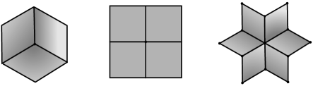
Fig. 10: Curvature about a vertex in a 2-d Euclidean cubical complex: positive, zero, and negative.

Such an extension of curvature to general metric spaces is made precise in Gromov’s work on curved metric spaces [13] (extending the classical work of Alexandrov, Busemann, and others) in which triangles with geodesic edges are used to measure curvature bounds. In brief, let $X$ be a metric space and $p\in X$ a point. To bound the curvature of $X$ at $p$, consider a small triangle $T$ about $p$ with geodesic edges of length $a$, $b$, and $c$. Build a comparison triangle $T^{\prime}$ in the Euclidean plane whose sides also have length $a$, $b$, and $c$ respectively. Choose a geodesic chord of $T$ and measure its length $d$. In $T^{\prime}$, measure the length $d^{\prime}$ of the chord whose endpoints correspond to those of the chord in $X$.

Definition 19.

A metric space $X$ is nonpositively curved (or NPC) if for every sufficiently small geodesic triangle $T$ and for every chord of $T$, it follows that $d\leq d^{\prime}$.

\psfragscanon\psfrag{a}{\Large{$a$}}\psfrag{b}{\Large{$b$}}\psfrag{c}{\Large{$c$}}\psfrag{d}{\Large{$d$}}\psfrag{A}{\Large{$a$}}\psfrag{B}{\Large{$b$}}\psfrag{C}{\Large{$c$}}\psfrag{D}{\Large{$d^{\prime}$}}\psfrag{X}{\Large{$X$}}\psfrag{E}{\Large{$\mathbb{R}^{2}$}}\includegraphics[angle={0},width=231.26378pt]{CAT0.ps}

Fig. 11: Comparison triangles measure curvature bounds.

In other words, geodesic chords are no longer than Euclidean comparison chords. It should be stressed that the NPC property is very special and highly desirable. Indeed, being NPC implies a variety of topological consequences reminiscent of smooth nonpositively curved manifolds.

Despite the variety of (local) metamorphic systems, all state complexes share this special geometric property.

Theorem 20.

The state complex ${\mathcal{S}}$ of any local metamorphic system is nonpositively curved.

The proof of this theorem is simple, but requires some additional machinery.

Definition 21.

Let $X$ denote a complex (either simplicial or cubical) and let $v$ denote a vertex of $X$. The link of $v$, $\ell k[{v}]$, is defined to be the abstract complex which has one $k$-dimensional simplex for each $(k+1)$-dimensional cube in $X$ incident to $v$. The boundary relations are those inherited from $X$: namely, the boundary of a $k$-simplex in $\ell k[{v}]$ represented by a $(k+1)$-cube in $X$ is the set of all simplices represented by the faces of the $(k+1)$-cube.

Links can be thought of as a simplicial version of the locus of points a small fixed distance from the vertex $v$.

Definition 22.

A Euclidean cube complex $X$ satisfies the link condition if, for each vertex $v\in X$, $\ell k[{v}]$ satisfies the following: for each $k$, if any $k+1$ vertices in $\ell k[{v}]$ are pairwise connected by edges in $\ell k[{v}]$, then those vertices bound a unique $k$-simplex in $\ell k[{v}]$.

An important and deep theorem of Gromov [13] asserts that a Euclidean cube complex is nonpositively curved if and only if it satisfies the link condition. This criterion makes it easy to prove Theorem 20.

proof of theorem 20:  Let ${U}$ denote a vertex of ${\mathcal{S}}$. Consider the link $\ell k[{{U}}]$. The 0-cells of the $\ell k[{{U}}]$ correspond to all edges in ${\mathcal{S}}$ incident to ${U}$; that is, actions of generators admissible at the state ${U}$. A $k$-cell of $\ell k[{{U}}]$ is thus a commuting set of $k+1$ of these actions based at ${U}$. The interpretation of the link condition for a state complex is as follows: if at ${U}$ one has a set of $k+1$ admissible actions, $\{({\mathbf{\phi}}_{\alpha_{i}},{\mathbf{\Phi}}_{\alpha_{i}})\}_{i=1}^{k+1}$, of which each pair commutes, then the full set of $k+1$ generators must commute [existence of the $k$-simplex in the link]. Furthermore, they must commute in a unique manner [uniqueness of the $k$-simplex in the link].

The proof of existence follows directly from Definition 8: any collection of pairwise commutative actions is totally commutative. We therefore have a $(k+1)$-dimensional cell in ${\mathcal{S}}$ which is the equivalence class $[{U};({\mathbf{\Phi}}_{\alpha_{i}})_{i=1}^{k+1}]$. This is the representative in ${\mathcal{S}}$ of the $k$-simplex in $\ell k[{{U}}]$. To show uniqueness, consider any other $k$-simplex in $\ell k[{{U}}]$ which has the same vertex set. This must correspond to a $(k+1)$-dimensional cube in ${\mathcal{S}}$ with actions $({\mathbf{\phi}}_{\alpha_{i}},{\mathbf{\Phi}}_{\alpha_{i}})_{i=1}^{k+1}$ (up to some permutation) based at ${U}$. From Definition 10, this cell must be the same equivalence class, namely $[{U};({\mathbf{\Phi}}_{\alpha_{i}})_{i=1}^{k+1}]$. ∎

Example 23.

To see how the NPC property can fail, consider the following non-local metamorphic system. Recall the generator for the planar hexagonal system presented in Fig. 2[right] which (along with its rotations) allows for local disconnection of the aggregate. If we add to this system a global rule that requires the aggregate to be connected (for, say, considerations of power transmission), then we no longer have a local system, and positive curvature may exist. Fig. 12 shows a configuration in which three actions of local generators act to disconnect the aggregate locally but not globally. These actions commute pairwise, and any two do not disconnect globally. However, performing all three actions disconnects the space and leads to an illegal state. Therefore, the corresponding state complex for this non-local system has a “corner” of positive curvature as a local factor. Note: the state complex will not be two-dimensional here, but will be locally a product of this with another cubical complex. The positive curvature persists.

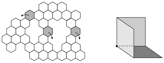
Fig. 12: A generator which allows for local disconnection [left] admits configurations [center] for which pairs of actions leave the aggregate connected, but triples do not; this non-local system has positive curvature in the state complex at this state [right].

7 Geodesics and time on ${\mathcal{S}}$

Besides displaying a unifying geometric feature, the nonpositive curvature has implications for path-planning, and hence, the shape-planning problem.

Corollary 24.

Each homotopy class of paths connecting two given points of a state complex contains a unique shortest path.

proof:   This is well-known for NPC spaces. The only difficulty lies in proving that the $d\leq d^{\prime}$ inequality for sufficiently small triangles implies the $d\leq d^{\prime}$ inequality for all geodesic triangles which are contractible in the space: see [5]. Assume, then, that this inequality holds in general, and consider a pair of distinct homotopic shortest paths from points $p$ to $q$ in ${\mathcal{S}}$. Choose any point $r$ on one of the two paths. The two halves of this path bisected by $r$ are themselves shortest paths from $p$ to $r$ and $r$ to $q$ respectively. Thus, there is a geodesic triangle in ${\mathcal{S}}$ whose comparison triangle in the Euclidean plane is a degenerate straight line from $p^{\prime}$ to $q^{\prime}$. The $d\leq d^{\prime}$ inequality applied to the segment from $r$ to its corresponding point on the other geodesic shows that these points coincide; therefore the two shortest paths from $p$ to $q$ in ${\mathcal{S}}$ are identical. ∎

Fig. 13[left] gives a simple example of a 2-d cubical complex with positive curvature for which the above corollary fails.

This corollary is a key ingredient in the applications of NPC geometry to path-planning on a configuration space, since one expects geodesics on ${\mathcal{S}}$ to coincide with optimal solutions to the shape planning problem. However, in the context of robotics applications, the goal of solving the shape-planning problem is not necessarily coincident with the geodesic problem on the state complex. Fig. 14[left] illustrates the matter concisely. Consider a portion of a state complex ${\mathcal{S}}$ which is planar and two-dimensional. To get from point $p$ to point $q$ in ${\mathcal{S}}$, any edge-path which is weakly monotone increasing in the horizontal and vertical directions is of minimal length in the transition graph. The true geodesic is, of course, the straight line, which is hardly a discrete object and thus more difficult to compute.

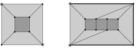
Fig. 13: [left] A 2-d cube-complex (with positive curvature) possessing distinct homotopic shortest paths between a pair of marked points — note all edges have length one; [right] a 2-d cube-complex (with positive curvature) possessing an edge path (the thick line on the boundary) which is a locally (but not globally) shortest path. Any cube path near this path is strictly longer.

Given the assumption that each elementary move can be executed at a uniform maximum rate, it is clear that the true geodesic on ${\mathcal{S}}$ is time-minimal in the sense that the elapsed time is minimal among all paths from $p$ to $q$. However, there is an envelope of non-geodesic paths which are yet time-minimizing. Indeed, the true geodesic in Fig. 14[left] “slows down” some of the moves unnecessarily in order to maintain the constant slope.

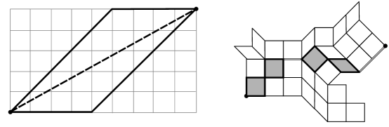
Fig. 14: [left] The true geodesic lies within an envelope of time-minimizing paths. No minimal edge-paths are time-minimizing; [right] a normal cube-path in an NPC complex (after [19]).

This leads us to define a second metric on ${\mathcal{S}}$, one which measures elapsed time. Namely, instead of the Euclidean metric on the cells of ${\mathcal{S}}$, consider the space ${\mathcal{S}}$ with the $\ell^{\infty}$ norm on each cell. (This is also called the supremum norm: a vector is measured by the maximum of its components in each coordinate direction.) The geodesics in this geometry represent reconfiguration paths which are time minimizing. Using the results of [19], one can prove that these geodesics are easily described using the notion of a cube path.

Definition 25.

A cube path from a vertex $v_{0}$ to a vertex $v_{N}$ is an ordered sequence of closed cubes $\{C_{i}\}_{1}^{N}$ in ${\mathcal{S}}$ which satisfy (1) $C_{i}\cap C_{i+1}=v_{i}$ for some vertex $v_{i}$; and (2) $C_{i}$ is the smallest cell of ${\mathcal{S}}$ containing $v_{i-1}$ and $v_{i}$. A cube path is said to be normal if in addition (3) for all $i$, ${\sf St}(C_{i})\cap C_{i+1}=v_{i}$, where ${\sf St}(C_{i})$ is the star of $C_{i}$ (the union of all closed cubes, including $C_{i}$, which have $C_{i}$ as a face).

Roughly speaking, a normal cube path is one which uses the highest dimensional cubes as early as possible in the path.

Theorem 26.

In any state complex ${\mathcal{S}}$, there exists a unique normal cube path from $p$ to $q$ in each homotopy class. The chain of diagonals through this cube path minimizes time among all paths in its homotopy class.

This result follows from Theorem 20 and a result of [19] (or, see the constructive algorithm of Section 8 below for a proof of existence).

This result (or, alternatively, the constructive algorithm in the next section) also implies that, in the category of homotopic cube-paths, there is no such thing as a strictly local minimum for length: if a cube path in ${\mathcal{S}}$ has the property that all nearby cube paths are longer (more cubes), then this cube path is a normal cube path and indeed is the shortest cube path within the homotopy class of paths. See Fig. 13[right] for a simple example of a cube complex with some positive curvature that has a cube path which is locally of minimal length among cube paths, but not globally so.

This is very significant. By beginning with any path in the state complex, say, one obtained via a fast distributed algorithm for shape-planning, one can employ a gradient-descent curve shortening on the level of cube paths. The above results imply that any algorithm which monotonically reduces length must converge to the shortest path (in that homotopy class) and cannot be hung up on a locally minimal cube path. The presence of local minima is a persistent problem in optimization schemes: nonpositive curvature is a handy antidote.

8 Optimizing paths

In cases where the state complex is sparse — local principal cells being of high dimension with few neighbors — it is possible to compress the size of the transition graph significantly. However, shape-planning via constructing all of ${\mathcal{S}}$ and determining geodesics is, in general, computationally infeasible: the total size of the state complex is often exponential in the number of cells in the aggregate. We therefore assume that some shape trajectory has been determined (by a perhaps ad hoc or distributed method) and turn to the problem of optimizing this trajectory. The nonpositive curvature of ${\mathcal{S}}$ allows for a time-optimization which does not require explicit construction of ${\mathcal{S}}$. We detail an algorithm for transforming any given edge-path to a time-optimal normal cube path.

From Definition 10, an $n$-dimensional cube $C$ of ${\mathcal{S}}$ can be represented by a set of $n$ commutative actions $\{{\mathbf{\Phi}}_{i}\}$ along with an admissible state ${U}$. In the following algorithm, we suppress the state for notational convenience and consider $C$ as the set of actions. Addition and subtraction is defined by adding or taking away admissible commutative actions to the list.

Algorithm 27 (TimeGeodesic).

Given: a cube path ${\mathcal{C}}=\{C_{i}\}_{i=1..N}$ in ${\mathcal{S}}$.

1:	Let $N:=$ Length$({\mathcal{C}})$.
2:	Call ShrinkCubePath$({\mathcal{C}})$.
3:	If Length$({\mathcal{C}})<N$ then 1: else stop.

Algorithm 28 (ShrinkCubePath).

Given: a cube path ${\mathcal{C}}=\{C_{i}\}_{i=1..N}$ in ${\mathcal{S}}$.

1:	Let $i=1$.
2:	Let $X:=$ Commute$(C_{i};C_{i+1})$.
3:	Update $C_{i}:=C_{i}+X$;
4:	Update $C_{i+1}:=C_{i+1}-X$.
5:	Call ExciseTrivial$(C_{i+1})$.
6:	Call CommonEdge$(C_{i-1},C_{i})$.
7:	Call ExciseTrivial$(C_{i-1};C_{i})$.
8:	If $X=\emptyset$ then $i=i+1$.
9:	If $C_{i+1}\neq\emptyset$ then 2: else stop.

Subroutine 29 (Commute).

Given: a pair of cubes $C_{j}=\{{\mathbf{\Phi}}^{j}_{\alpha_{i}}\}_{i=1..m}$ and $C_{j+1}=\{{\mathbf{\Phi}}^{j+1}_{\beta_{i}}\}_{i=1..n}$,

1:	Let $S:=\bigcup_{i}{\mbox{\sc sup}}({\mathbf{\Phi}}_{\alpha_{i}}^{j})$
2:	Let $T:=\bigcup_{i}{\mbox{\sc tr}}({\mathbf{\Phi}}_{\alpha_{i}}^{j})$
3:	For $i=1..n$ return ${\mathbf{\Phi}}^{j+1}_{\beta_{i}}$ if
	3.1: $S\cap{\mbox{\sc tr}}({\mathbf{\Phi}}^{j+1}_{\beta_{i}})=\emptyset$ ; and
	3.2: $T\cap{\mbox{\sc sup}}({\mathbf{\Phi}}^{j+1}_{\beta_{i}})=\emptyset$.

Subroutine ExciseTrivial checks a cube for an empty list, removes these from the path, and reindexes the cube path, thus reducing the length. Subroutine CommonEdge checks a cube against adjacent cubes in the sequence for common edges and deletes these, returning a genuine cube path (recall Definition 25).

Subroutine Commute takes as its argument a pair of cubes $C_{i}$ and $C_{i+1}$ and returns those elements of $C_{i+1}$ which commute with all elements of $C_{i}$. The following lemma is a manipulation of the definitions.

Lemma 30.

The result of Commute$(C_{i};C_{i+1})$ is precisely the set of edges in ${\sf St}(C_{i})\cap C_{i+1}$.

\psfragscanon\psfrag{1}{\Large{${\mathcal{C}}$}}\psfrag{2}{\Large{$1$}}\psfrag{3}{\Large{$2$}}\psfrag{4}{\Large{$3$}}\includegraphics[angle={0},width=252.94499pt]{algorithm.ps}

Fig. 15: Three rounds of shortening an edge path ${\mathcal{C}}$. Cube path length stabilizes after two calls to ShrinkCubePath. Three more calls produces a normal cube path.

Theorem 31.

Given a cube path ${\mathcal{C}}$, Algorithm 27 computes a globally time-optimal path in the homotopy class of ${\mathcal{C}}$.

proof:   Recall that in this setting, the length of a cube path refers to the number of cubes in the path; this equals the time required to execute the reconfiguration.

Repeated calls to Algorithm ShrinkCubePath eventually leave a cube path fixed. To show this, note that the integer-valued function $f({\mathcal{C}}):=\sum_{i}i\cdot\dim(C_{i})$ decreases in each call to ShrinkCubePath which changes the path. Lemma 30 implies that ShrinkCubePath leaves a cube path fixed if and only if it is a normal cube path. From Theorem 26, this yields a time-optimal path.

However, Algorithm TimeGeodesic calls ShrinkCubePath only until the length of the cube path is unchanged. Thus it remains to show that once the length of a cube path in unchanged by a call to ShrinkCubePath, this is equal to the length of the associated normal cube path. To show this, assume that ShrinkCubePath stops without excising any trivial cubes (i.e., shortening the length). We show that further calls merely redistribute actions earlier in the list ${\mathcal{C}}$ without deleting any permanently. Without a loss of generality, assume that the first call to ShrinkCubePath does not change the length of the cube path, but that in the subsequent call, the cube $C_{i+1}$ is eliminated via $C_{i}$ commuting with a portion of $C_{i-1}$: see the schematic of Fig. 16.

\psfragscanon\psfrag{k}{\Large{$C_{i+1}$}}\psfrag{i}{\Large{$C_{i-1}$}}\psfrag{j}{\Large{$C_{i}$}}\psfrag{E}{\Large{$=$}}\includegraphics[angle={0},width=187.90244pt]{exchange.ps}

Fig. 16: Schematic of exchanging actions in sequential rounds. Each dimension in this cartoon represents a multi-dimensional cube.

Since $C_{i+1}$ is not eliminated in the first call, there must have been actions in $C_{i}$ which did not commute with those of $C_{i-1}$ but which are subsequently pushed backward in the second call. In addition, all the actions of $C_{i+1}$ are contained in (“parallel to” in the figure) the subset of $C_{i-1}$ which commutes with $C_{i}$ in the second call. This being the case, the commutativity of $C_{i+1}$ with $C_{i}$ would have occurred in the first call: contradiction. ∎

It is not surprising that Algorithm 27 converges to a locally time-minimal solution. The interesting implication is that the cube-path obtained is the global minimum for all paths obtainable from the initial: there is no way to get a quicker reconfiguration path by first lengthening the path and then shortening. This is the boon of nonpositive curvature. Fig. 15 gives an example of paths generated by Algorithm 27.

The complexity of Algorithm 27 depends on both the catalogue of generators for the system and the length $N$ of the input edge path. However, the dependence on the catalogue arises only in Subroutine Commute, which tests various pairs of subsets of the workspace for disjointness; the sizes of these subsets are governed by the generators. Assuming a fixed catalogue, then, there is a constant bound on the time required for a single call to Commute, and we may analyze the complexity of Algorithm 27 as a function of $N$ alone.

Notice that Algorithm 27 calls ShrinkCubePath at most $N$ times, since it stops as soon as the length of the cube path fails to decrease. Each time an individual loop of ShrinkCubePath is executed, the quantity $\sum\dim(C_{j})$ decreases. Since this quantity equals $N$ initially, ShrinkCubePath calls the subroutines Commute, ExciseTrivial, and CommonEdge each at most $N$ times. Each of these has a constant running time, with Commute being the only one depending on the particulars of the metamorphic system. Therefore the complexity of the entire Algorithm 27 is $O(N^{2})$, with the constant determined by the running time of Commute.

The worst case for Algorithm 27 seems to be achieved in a totally flat 2-d state complex by a path consisting of two perpendicular segments of length $N/2$. (This case requires $N^{2}/2$ runs of ShrinkCubePath.) The presence of true negative curvature in a state complex greatly increases the speed of convergence. On the other hand, a flat state complex is desirable for other reasons.

It remains an important computational question to determine whether the homotopy class of the initial path (given, say, from a distributed algorithm) is optimal in the sense that its geodesic is the shortest among all homotopy classes. Interestingly, in contrast to the previous paragraph, this problem becomes quite a bit more difficult in the presence of negative curvature. From this point of view it is preferable to have a flat state complex.

9 Discussion

Our principal contributions are:

1. A mathematical definition of a metamorphic system which encompass many models currently studied and suggests seemingly unrelated (and often simpler) systems. Given the difficulty of building large metamorphic systems, simpler examples possessing the same formal structure may be valuable.

2. The state complex, whose naturality is manifested on the level of its topology (${\mathcal{S}}$ can be homotopically simple) and its geometry (non-positive curvature is universal, mathematically helpful, and highly desirable for shape planning).

There are drawbacks to this approach. Primary among them are the dual dilemmas that shape planning is inherently complex, and that there are many types of reconfiguration possible. A state complex approach is not meant for all systems. Indeed, it is possible to design degenerate metamorphic systems with little to no commutativity. Nevertheless, paying attention to the geometry lurking behind our higher-dimensional versions of transition graphs leads to a nontrivial result on the optimality of path-shortening.

As an interesting side-note, we observe that in the present context, the optimal reconfiguration path is not always coincident with a geodesic on the configuration space. This principle holds in more generality.

Finally, in this initial work, we have focused only on the first-order problem of shape planning. We hope that the mathematical framework here suggested finds uses in more sophisticated task-planning problems for metamorphic and reconfigurable robots.

Appendix A Shape complexes

State complexes, despite their relative simplicity over the transition graph, nevertheless typically contain a large number of cells. For lattice-based systems, and in some other cases as well, a much smaller complex called the shape complex can be used to encode all of the local reconfigurations, without losing any essential information from the state complex. The idea is to exploit the symmetries of the domain.

Consider the (lattice-based) pivoting hex system of Example 4. The underlying lattice has translational symmetry in two independent directions; so for instance, in the idealized case where the workspace is the entire (infinite) lattice with no obstacles, the state complex ${\mathcal{S}}$ shares these symmetries. If we take a quotient of ${\mathcal{S}}$ by the actions of these two translations, we obtain the shape complex ${\mathcal{S}h}$. (The precise definition follows shortly.)

Observe that ${\mathcal{S}h}$ is much smaller than ${\mathcal{S}}$; indeed even if the workspace is infinite, the complex ${\mathcal{S}h}$ is compact (provided the system consists of connected sets of, say, $N$ cells). Yet, ${\mathcal{S}h}$ carries substantially the same information as ${\mathcal{S}}$. Whereas ${\mathcal{S}}$ keeps track of both the shape and the location of the aggregate, the quotient ${\mathcal{S}h}$ ignores the location.

Note that no information about the system is lost in the process of forming the quotient; ${\mathcal{S}}$ can be completely reconstructed from ${\mathcal{S}h}$. Indeed, ${\mathcal{S}}$ is a covering space of ${\mathcal{S}h}$ (with covering transformation group equal to the group of symmetries of the lattice). In particular ${\mathcal{S}h}$ and ${\mathcal{S}}$ share the same universal covering space, so ${\mathcal{S}h}$ (just like ${\mathcal{S}}$) is non-positively curved.

Here is the definition of the shape complex; compare with Definition 10.

Definition 32.

The shape complex ${\mathcal{S}h}$ of a (lattice-based) local reconfigurable system is the abstract cube complex whose $k$-dimensional cubes are equivalence classes $[{U};(\Phi_{\alpha_{i}})_{i=1}^{k}]$ where

1. $(\Phi_{\alpha_{i}})_{i=1}^{k}$ is a $k$-tuple of commuting actions of generators $\phi_{\alpha_{i}}$;

2. ${U}$ is some state for which all the actions $(\Phi_{\alpha_{i}})_{i=1}^{k}$ are admissible; and

3. $[{U}_{0};(\Phi_{\alpha_{i}})_{i=1}^{k}]=[{U}_{1};(\Phi_{\beta_{i}})_{i=1}^{k}]$ if and only if there is a translation $T:{\mathcal{L}}\to{\mathcal{L}}$ such that the list $(\Phi_{\beta_{i}}\circ T)$ is a permutation of $(\Phi_{\alpha_{i}})$, and ${U}_{0}={U}_{1}\circ T$ on the set ${\mathcal{W}}-\bigcup_{i}\Phi_{\alpha_{i}}({\mbox{\sc sup}}({\mathbf{\phi}}_{\alpha_{i}}))$ .

The boundary of a $k$-cube is obtained just as it is in ${\mathcal{S}}$.

Example 33.

The shape complex for the system of Example 4 (with the generator of Fig. 2[left]) having a total of $N=3$ occupied cells is shown in Figure 17. There are nine square cells. Two pairs of edges are identified according to the matching arrows, yielding a Mobius strip; additionally, the three black vertices are identified to one, as are the three white vertices. The shape complex is therefore a Mobius strip with some of the boundary points identified.

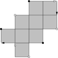
Fig. 17: The shape complex for a pivoting hex system consisting of 3 robotic cells.

Macros. The most obvious advantage of the shape complex is that the discovery of a single shortest path in ${\mathcal{S}h}$ simultaneously solves several state-changing problems in the complex ${\mathcal{S}}$. This is particularly helpful in systems which require frequent transportation within the workspace (perhaps to perform various tasks in different areas). For instance, suppose the workspace includes several narrow corridors through which the robot must travel at various times. At each encounter with such a corridor, it must change to a shape which is skinny enough to navigate the passageway. But this is the same problem at each corridor, even though it occurs in different places in the state complex: the three hexagons in Example 33 can move from a triangular shape to a linear shape by the same sequence of moves, wherever the problem may arise in ${\mathcal{L}}$.

In the shape complex, we view this as a single shortest-path problem, whose solution we may lift to various locations in the domain. In this sense a shortest path $P$ in ${\mathcal{S}h}$ can be viewed as a macro for solving state-changing problems in ${\mathcal{S}}$.

A drawback to the shape complex is that it neglects the shape of the workspace ${\mathcal{W}}$. In the presence of obstacles or at the edge of ${\mathcal{W}}$, a path $P$ in ${\mathcal{S}h}$ may fail to lift to a path in ${\mathcal{S}}$. Thus before lifting a path $P$ one must check that the actions are admissible at the appropriate locations in ${\mathcal{W}}$.

References

- [1]
- [2] A. Abrams, Configuration spaces and braid groups of graphs. Ph.D. thesis, UC Berkeley, 2000.
- [3] A. Abrams and R. Ghrist, Finding topology in a factory: configuration spaces, Amer. Math. Monthly (109), 140–150, 2002.
- [4] A. Abrams and R. Ghrist, Cubical complexes for reconfigurable systems, in preparation.
- [5] M. Bridson and A. Haefliger, Metric Spaces of Nonpositive Curvature, Springer-Verlag, Berlin, 1999.
- [6] Z. Butler, S. Byrnes, and D. Rus, Distributed motion planning for modular robots with unit-compressible modules, in Proc. IROS 2001.
- [7] Z. Butler, K. Kotay, D. Rus, and K. Tomita, Cellular automata for decentralized control of self-reconfigurable robots, in Proc. IEEE ICRA Workshop on Modular Robots, 2001.
- [8] G. Chirikjian, Kinematics of a metamorphic robotic system, in Proc. IEEE ICRA, 1994.
- [9] G. Chirikjian and A. Pamecha, Bounds for self-reconfiguration of metamorphic robots, in Proc. IEEE ICRA, 1996.
- [10] D. Epstein et al., Word Processing in Groups. Jones & Bartlett Publishers, Boston MA, 1992.
- [11] R. Ghrist, Configuration spaces and braid groups on graphs in robotics, AMS/IP Studies in Mathematics volume 24, 29-40, 2001.
- [12] R. Ghrist and D. Koditschek, Safe cooperative robot dynamics on graphs, SIAM J. Cont. & Opt. 40(5), 1556–1575, 2002.
- [13] M. Gromov, Hyperbolic groups, in Essays in Group Theory, MSRI Publ. 8, Springer-Verlag, 1987.
- [14] K. Kotay and D. Rus, The self-reconfiguring robotic molecule: design and control algorithms, in Proc. WAFR, 1998.
- [15] C. McGray and D. Rus, Self-reconfigurable molecule robots as 3-d metamorphic robots, in Proc. Intl. Conf. Intelligent Robots & Design, 2000.
- [16] S. Murata, H. Kurokawa, and S. Kokaji, Self-assembling machine, in Proc. IEEE ICRA, 1994.
- [17] S. Murata, H. Kurokawa, E. Yoshida, K. Tomita, and S. Kokaji, A 3-d self-reconfigurable structure, in Proc. IEEE ICRA, 1998.
- [18] A. Nguyen, L. Guibas, and M. Yim, Controlled module density helps reconfiguration planning, in Proc. WAFR, 2000.
- [19] G. Niblo and L. Reeves, The geometry of cube complexes and the complexity of their fundamental groups, Topology, 37(3), 621-633, 1998.
- [20] A. Pamecha, I. Ebert-Uphoff, and G. Chirikjian, Useful metric for modular robot motion planning, in IEEE Trans. Robotics & Automation, 13(4), 531-545, 1997.
- [21] J. Walter, J. Welch, and N. Amato, Distributed reconfiguration of metamorphic robot chains, in Proc. ACM Symp. on Distributed Computing, 2000.
- [22] J. Walter, E. Tsai, and N. Amato, Choosing good paths for fast distributed reconfiguration of hexagonal metamorphic robots. In Proc. IEEE ICRA, 2002.
- [23] M. Yim, A reconfigurable robot with many modes of locomotion, in Proc. Intl. Conf. Adv. Mechatronics, 1993.
- [24] M. Yim, J. Lamping, E. Mao, and J. Chase, Rhombic dodecahedron shape for self-assembling robots, Xerox PARC Tech. Rept. P9710777, 1997.
- [25] Y. Zhang, M. Yim, J. Lamping, and E. Mao, Distributed control for 3-d shape metamorphosis, Aut. Robots. J., 41-56, 2001.
- [26] E. Yoshida, S. Murata, K. Tomita, H. Kurokawa, and S. Kokaji, Distributed formation control of a modular mechanical system, in Proc. Intl. Conf. Intelligent Robots & Sys., 1997.