Sharp Bounds for Bandwidth of Clique Products

Abstract

The bandwidth of a graph is the labeling of vertices with minimum maximum edge difference. For many graph families this is NP-complete. A classic result computes the bandwidth for the hypercube. We generalize this result to give sharp lower bounds for products of cliques. This problem turns out to be equivalent to one in communication over multiple channels in which channels can fail and the information sent over those channels is lost. The goal is to create an encoding that minimizes the difference between the received and the original information while having as little redundancy as possible. Berger-Wolf and Reingold [2] have considered the problem for the equal size cliques (or equal capacity channels). This paper presents a tight lower bound and an algorithm for constructing the labeling for the product of any number of arbitrary size cliques.

Abstract

Key words. Graph bandwidth, hamming graph, cartesian products of cliques, complete graphs, algorithm design.

Key words. Graph bandwidth, hamming graph, cartesian products of cliques, complete graphs, algorithm design.

1 Introduction

Labeling of graph vertices is an active area of research related to many applications ranging from VLSI to computational biology. There are several graph parameters associated with a labeling that can be optimized. One such is bandwidth, the maximum difference between labels on an edge. In general, bandwidth of a graph is an NP-complete problem [10]. Even for very restricted families, e.g. trees of maximum degree 3 or varieties of caterpillars, it remains NP-complete. In this paper we focus on the bandwidth of Hamming graphs – cartesian product of cliques. Applications of this specific problems arise in designing encodings for packet-switched networks that minimize the error in case of packet loss [1, 8, 9, 11].

1.1 Problem Statement

Given a graph, $G=(V,E)$, a labeling $f$ of a graph is an assignment of numbers $\{1,...,|V|\}$ to the graph’s vertices:

$$f:V\to\{1,...,|V|\}$$

A labeling $f$ is a bijection.

Given a labeling, bandwidth is the maximum over all edges of the difference between labels on an edge:

$$B_{f}(G)=\max_{\langle u,v\rangle\in E}{\{|f(u)-f(v)|\}}$$

Graph bandwidth is the minimum possible bandwidth of a graph:

$$B(G)=\min_{f}{\{B_{f}(G)\}}$$

The Bandwidth Optimization problem is the problem of finding a labeling that minimizes the graph bandwidth. As we have mentioned, for a general graph, the bandwidth optimization problem is NP-hard [10].

A cartesian product of two graphs $G_{1}=(V_{1},E_{1})$ and $G_{2}=(V_{2},E_{2})$ is a graph whose vertices are tuples of the original vertices, and whose edges go between vertex tuples different in only one coordinate:

$$G_{1}\times G_{2}=\left({\begin{array}[]{c}V=\{(v_{1},v_{2}):v_{1}\in V_{1},v_{2}\in V_{2}\},\\ E=\{\langle(v_{1},v_{2}),(u_{1},u_{2})\rangle:v_{1}=u_{1}\wedge\langle v_{2},u_{2}\rangle\in E_{2}\mbox{ or }\langle v_{1},u_{1}\rangle\in E_{1}\wedge v_{2}=u_{2}\}\end{array}}\right)$$

A cartesian product can be inductively extended to more than two graphs.

A clique $K_{n}$ is a simple undirected graph on $n$ vertices with ${n\choose 2}$ edges, an edge between every vertex pair. Given $d$ complete graphs (cliques) $K_{n_{1}},...,K_{n_{d}}$, a Hamming graph is their cartesian product $K_{n_{1}}\times\cdots\times K_{n_{d}}$.

We first consider the product of two cliques of unequal order. We prove a tight lower bound on the graph bandwidth and give an optimal algorithm that achieves that lower bound. We generalize the results for arbitrary number of cliques. To the best of our knowledge, this is the first result for bandwidth optimization of products of cliques of unequal order.

1.2 Problem Background

In graph theory, the bandwidth problem was introduced by Harper in 1966 [5], where he solved the problem for hypercubes, that is products of $K_{2}$’s. Hendrich and Stiebitz [7] solved the bandwidth problem for products of two cliques of equal size. In [6] Harper gives a non-constructive asymptotically best lower bound for products of cliques of equal sizes. Berger-Wolf and Reingold [2] have introduced a general technique that gives a lower bound and an algorithm for $d$-fold products of cliques of equal sizes. While their technique is applicable to cliques of unequal sizes, the lower bound is very loose in that case. Here we propose a new and simple technique for deriving a tight lower bound and give an optimal algorithm for the the case of unequal size cliques.

2 Results

We present a technique that provides a lower bound for the bandwidth of the Hamming graph as a maximum of lower bounds for each clique. The technique also suggests an algorithm which provides an almost matching upper bound and is thus nearly optimal. The minimal bandwidth is

$$B(K_{n_{1}}\times K_{n_{2}}\times\dots\times K_{n_{d}})=\Theta(B(K_{2}^{d})\times\prod{n_{t}\over 2}),$$

where $B(K_{2}^{d})=\sum_{t=0}^{d-1}{t\choose\lfloor{t/2}\rfloor}$ is the bandwidth of the product of $d$ $2$-cliques.

The problem of minimizing the bandwidth of $K_{n_{1}}\times K_{n_{2}}\times\cdots\times K_{n_{d}}$ can be thought of as the problem of arrangement of numbers $\{1,\dots,\prod{n_{t}}\}$ in an $n_{1}\times n_{2}\times\cdots\times n_{d}$ matrix in a way that minimizes the maximum difference between the largest and the smallest number in any line – a full one-dimensional submatrix. The correspondence is straightforward; the numbers within a line represent vertices within the same clique and so a minimizing arrangement minimizes the bandwidth.

Figure 1 shows the correspondence between the two problems in case of two dimensions. We assume throughout this paper without loss of generality that $n_{1}\leq n_{2}\leq\cdots\leq n_{d}$.

Figure 1: Correspondence between the number arrangement of a two-dimensional matrix and the bandwidth minimization of a product of two cliques problems.

We first show a lower bound for the problem and then present an algorithm that nearly achieves that lower bound. After giving the fundamental lemmata we demonstrate the approach for the two-dimensional case and the generalize it to arbitrary dimensions.

Definition 1

Let an arrangement be a one-to-one function $A:{\mathcal{N}}\to{\mathcal{N}}^{d}$ from $\{1,\dots,\prod_{t=1}^{d}{n_{t}}\}$ onto the set of cells of an $n_{1}\times n_{2}\times\cdots\times n_{d}$ matrix. Let a line be a full one-dimensional submatrix of the type $(i_{1},i_{2},...,*,...,i_{d})$ with all but one coordinate fixed. Then the spread of an arrangement is the maximum difference over all lines between any two numbers in any line:

$${\rm spread}(A)=\max_{1\leq i_{t},j_{t}\leq n_{t},1\leq t\leq d\atop s\neq t\rightarrow i_{s}=j_{s}}{|A^{-1}(i_{1},i_{2},...,i_{t},...,i_{d})-A^{-1}(j_{1},j_{2},...,j_{t},...,j_{d})|}.$$

Since $A$ is a bijection, to simplify the notation, we will use $A$ and $A^{-1}$ interchangeably, the meaning hopefully being clear from the context.

First, we note that the lower bound on the spread for any line is the lower bound on the spread in the entire matrix, therefore the maximum of the line bounds is also a lower bound for the matrix spread. Thus we can deal with one line at a time. We then restrict our attention to a special kind of arrangement showing that this restriction does not eliminate optimal arrangements. Then for these arrangements it is easier to find a line with a large spread.

Definition 2

An arrangement is monotonic if the values in any line ascend with the increase of the changing coordinate. That is, an arrangement $A$ is monotonic if for all $1\leq i_{t},j_{t}\leq n_{t},\>1\leq t\leq d$

$$((s\neq t\rightarrow i_{s}=j_{s})\wedge i_{t}<j_{t})\rightarrow A(i_{1},...,i_{t},...,i_{d})<A(j_{1},...,j_{t},...,j_{d}).$$

Lemma 2.1

Given any arrangement of any set of $n_{1}n_{2}\cdots n_{d}$ numbers, sorting it to become monotonic one coordinate at a time, one line at a time, does not increase the spread. That is, for any arrangement $A$,

$${\rm spread}({\rm sorted}(A))\leq{\rm spread}(A).$$

Proof. We first show that given any arrangement, sorting the numbers to become monotonic in one coordinate does not increase the overall spread. It is obvious that rearranging the numbers in any way within the same line does not change the spread in that line, thus sorting within a coordinate does not change the spread in that coordinate. Suppose the spread has increased in another coordinate. The situation is illustrated in Figure 2. Let the maximum spread in that coordinate after sorting be $b_{t}-a_{s}$ appearing in line $j$ (where $b_{t}$ was in line $t$ before the rearrangement, and $a_{s}$ was in line $s$). Then

$$|b_{t}-a_{t}|<b_{t}-a_{s},\mbox{ thus }a_{s}<a_{t},\mbox{ and}$$

$$|b_{s}-a_{s}|<b_{t}-a_{s},\mbox{ thus }b_{s}<b_{t}.$$

Then there are $j-2$ (since $b_{t}$ and $a_{s}$ are now in line $j$) $b$’s less than $b_{t}$ and not equal to $b_{s}$. There are $j-1$ $a$’s less than $a_{s}$ and not equal to $a_{t}$. Therefore, by the pigeonhole principle, there exists $a_{p}<a_{s}$ that was paired up with $b_{p}>b_{t}$ before the rearrangement. But then $b_{p}-a_{p}>b_{t}-a_{s}$, which contradicts the assumption that the spread increased after sorting. Thus sorting in one coordinate does not increase the spread in any coordinate.

Figure 2: Sorting the values within the rows causes the spread in columns to increase to $b_{t}-a_{s}$, occurring now in column $j$. Before sorting, $b_{t}$ was in column $t$ and $a_{s}$ was in column $s$. Shaded are the $c$’s less than $a_{s}$ but not equal to $a_{t}$ and $b$’s that are less than $b_{t}$ and not equal to $b_{s}$. Note that necessarily $s<t$, but $j$ can be any column relative to $s$ and $t$.

Gale and Karp [4] show that if the arrangement was monotonic in any coordinate then it will remain so after the numbers are sorted in any other coordinate. Thus the matrix can be sorted to have a monotonic arrangement one coordinate at a time, one line at a time, without increasing the spread.        

This allows us to restrict attention to monotonic arrangements. From these arrangements we can more easily find a general structure of the lower bound on the spread.

Consider some number $x$ in a cell of a monotonic arrangement. The $d$ axis-parallel hyperplanes that pass through that cell divide the matrix into $2^{d}$ orthants. For any monotonic arrangement of any set of $n_{1}n_{2}\cdots n_{d}$ numbers, all the numbers in the orthant containing the coordinate $(1,1,...,1)$ are necessarily less than $x$, and all the numbers in the orthant containing the last coordinate are necessarily greater than $x$. Besides the first and the last orthants, the other $2^{d}-2$ orthants may contain both numbers less than and greater than $x$. Any line passing through $x$ necessarily has both numbers less and greater than $x$ by the nature of monotonicity of the arrangement. However any other line can be filled entirely with only smaller or larger numbers.

Lemma 2.2

For the optimal arrangement $A$ of numbers $1,...,\prod_{t=1}^{d}{n_{t}}$ in an $n_{1}\times n_{2}\times...\times n_{d}$ matrix, there exists a line $(i_{1},i_{2},...,i_{j-1},*,i_{j+1},...,i_{d})$ (all the coordinates but the $j$th are fixed) in that arrangement and there exists a cell in that line $(i_{1},i_{2},...,i_{j},...,i_{d})$ such that the spread in that line is at least the volume of any minimal set of orthants (as defined by the cell) that separates between the orthant containing the cell $(1,..,1)$ (the first orthant) and the orthant containing the cell $(n_{1},...,n_{d})$ (the last orthant).

Proof. First, we will note several facts:

• Removing any minimal separating set of orthants leaves only two connected sets of orthants: the set containing the first orthant (we shall call this set “small” orthants) and the set containing the last orthant (“large” orthants).

• Since the set is a minimal separating set, any cell within any of the separating orthants is contained in lines that intersect the “large” orthants and in lines that intersect the “small” orthants.

• No line passes through both the “small” and “large” orthants, since otherwise they would not be separated.

Now we are ready to prove the lemma. Let $V_{small}(cell)$ be the volume (number of cells) of the “small” orthants, $V_{large}(cell)$ be the volume of the “large” orthants, and $V_{sep}(cell)$ be the volume of the separating orthants. Note that $V_{small}+V_{sep}+V_{large}=\prod_{t=1}^{d}{n_{t}}=V$. For the optimal arrangement $A$ let $l=(i_{1},i_{2},...,*,...,i_{d})$ be the line with the largest spread (that is, the spread of the arrangement is the spread in this line). Here are the two possible cases:

• there exists a cell $(i_{1},i_{2},...,i_{j},...,i_{d})$ such that the smallest number in the line, $\min_{l}$, is at most $V_{small}(cell)$ (for any separating set defined by the cell), and the largest number in the line, $\max_{l}$, is at least $V-V_{large}(cell)$. Then

  $${\rm spread}(A) \geq {\rm max}_{l}-{\rm min}_{l}$$

  $$\geq V-V_{large}(cell)-V_{small}(cell)$$

  $$= V_{sep}(cell)$$

  and the statement of the lemma holds.

• for all cells in the line, for some separating set for each cell, either $\max_{l}<V-V_{large}$ or $\min_{l}>V_{small}$.
  

  Let $i_{j}$ be such that $V_{sep}$ as defined by $(i_{1},...,i_{j},...,i_{d})$ is the smallest. Without loss of generality we assume that $\min_{l}>V_{small}(i_{1},...,i_{j},...,i_{d})$, while $\max_{l}$ can be either less or greater or equal to $V-V_{large}(i_{1},...,i_{j},...,i_{d})$.

  Since $\min_{l}>V_{small}(i_{1},...,i_{j},...,i_{d})$ there must be at least one element less than $\min_{l}$ in the separating orthants defined by the cell $(i_{1},...,i_{j},...,i_{d})$. Suppose there are $s$ elements that are less than $\min_{l}$ total in the separating orthants. Then there are at most $s-1$ elements greater than $\min_{l}$ in the small orthants. Each of the $s$ elements in the separating orthants must be in a line that intersects large orthants (as defined by the cell $(i_{1},...,i_{j},...,i_{d})$). Since $\max_{l}-\min_{l}$ is the largest spread, all elements in those lines must be less than $\max_{l}$. Let there be $l$ of those elements. One possible way this can happen is shown in Figure 3.

  

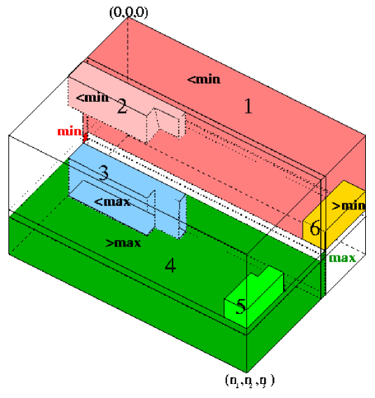
  Figure 3: Areas (1) and (6) are the small orthants, areas (4) and (3) are the large orthants, and the uncolored area, with (2) and (5), are the separating orthants. The indicated min and max are the minimum and maximum in the line $l$. (1) are the numbers less than $\min_{l}$ in the small orthants. (2) are the $s$ numbers less than $\min_{l}$ in the separating orthants. (3) are the $l$ numbers less than $\max_{l}$ in the large orthants. Those are the intersection of the lines that have a light red minimum with the large orthants. (4) are the numbers greater than $\max_{l}$ in the large orthants. (5) are the $p$ numbers greater than $\max_{l}$ in the separating orthants. (6) are the matching numbers greater than $\min_{l}$ in the small orthants.

  We use a switching idea similar to Fishburn, Tetali, and Winkler [3]. Suppose there are $t\geq l$ elements total less than $max_{l}$ in the large orthants. Then $max_{l}\leq V-V_{large}+t$. Replace the largest of those $t$ elements $l_{1}$ with $max_{l}$, then replace the next largest element $l_{2}$ with $l_{1}$ and so on, trickling down until we get to the smallest of those $t$ elements. Put that smallest element instead of $max_{l}$. We have not violated the monotonicity. We have increased each of the $t$ elements by at least $1$ and decreased $max_{l}$ by $t$. Therefore the new $max_{l}\leq V-V_{large}$ and all the elements in the large orthants are greater than $max_{l}$. Similarly, we can replace the largest of the $s$ small elements, $s_{1}$, with $min_{l}$, then replace the next largest element $s_{2}$ with $s_{1}$, and so on until we either reach the $t$th largest or the smallest of the $s$ elements. We replace $min_{l}$ with that element. We have increased each of the $s$ elements by at most $1$, so the relative spread has not increased. The minimum $min_{l}$ has decreased by at most $t$, so the spread in line $l$ has not increased.

  If $s>t$ then we have stopped after replacing $t$ of the $s$ elements and there are still some elements less than the new $min_{l}$ in the separating orthants in the lines with elements greater than the new $max_{l}$. We have not increased the spread in line $l$ or anywhere else, but the spread in those lines is greater than the new $max_{l}-min_{l}$ which equals the old spread since both the minimum and the maximum decreased by the same amount. This is a contradiction to the assumption that $l$ was the line with the maximum spread.

  If $s\leq t$ then there are no elements less than $min_{l}$ in the separating orthants and the new $min_{l}\leq V_{small}$. If there are no elements greater than $max_{l}$ in the separating orthants, then $max_{l}-min_{l}\geq V_{sep}$, which means the initial spread was also at least $V_{sep}$, which is a contradiction. Suppose there are $p$ elements greater than the new $max_{l}$ in the separating orthants. Those elements must be in lines that intersect small orthants and the elements in the small orthants in those lines must be greater than the new $min_{l}$. Suppose there are $q$ of those elements. We can perform the same replacement procedure and if $p>q$ we will get the same contradiction as in case of $s>t$. Otherwise, $p\leq q$. Since there are no elements less than the new $min_{l}$ in the separating orthants and there are $q$ elements in the small orthants that are greater than $min_{l}$, then the new $min_{l}=V_{small}-q$ and therefore the original $min_{l}=V_{small}-q+s$. Similarly, since there are $p$ elements greater than the new $max_{l}$ in the separating orthants and no elements less than it in the large orthants, the new $max_{l}=V-V_{large}-p$ and thus the original $max_{l}=V-V_{large}-p+t$. So the original spread is the difference between the original $\max_{l}$ and $\min_{l}$ which is

  $$(V-V_{large}-p+t)-(V_{small}-q+s)=V_{sep}+q-p+s-t.$$

  Since $p\leq q$ and $s\leq t$, the original spread was at least $V_{sep}$, which is, again, a contradiction.

Therefore, the spread in an optimal arrangement is at least $V_{sep}$ for any minimal set of the separating orthants as defined by some cell in the maximum spread line.

     

We have proved that the spread in an optimal arrangement is at least the volume of any minimal set of orthants separating between the “small” and “large” orthants, for some cell in the largest spread line. Therefore, there is a cell such that the spread is at least the volume of the largest minimal separating set of orthants, the one that has the largest number of orthants. In fact, if we associate a super vertex with each orthant and have an edge between any two vertices if the corresponding orthants are adjacent, then we get a $d$-dimensional hypercube representing the orthants. Figure 4 shows this in $3$ dimensions.

Figure 4: Correspondence between the orthants and a hypercube in $3$ dimensions. The $small(x)$ and $large(x)$ numbers meet only if a line passes through two adjacent orthants.

By definition of bandwidth, the largest minimum separating set of orthants is exactly the bandwidth of the $d$-dimensional hypercube. So for an optimal arrangement, for any line in the arrangement, the spread is at least the minimum over all cells of the volume of the bandwidth-separating set of orthants. Thus the spread in the optimal arrangement is at least

$$\max_{\mbox{all lines}}{\{\min_{\mbox{cells in a line}}{\{\min_{\mbox{separating set }\atop\mbox{of }B(K_{2}^{d})\mbox{ orthants}}{\{\mbox{volume of the separating set of orthants}\}}\}}\}}.$$

Using this lemma we can calculate the lower bound on the spread in the optimal arrangement. We will first demonstrate our approach in two dimensions and then generalize is to arbitrary number of dimensions.

2.1 Two Dimensions

Theorem 2.1

Without loss of generality assume $n_{1}\leq n_{2}$. The spread in any arrangement of an $n_{1}$ by $n_{2}$ matrix is at least

$${(n_{1}+1)n_{2}\over 2}-1\mbox{ if }n_{1}\mbox{ is odd, }$$

$${n_{1}(n_{2}+1)\over 2}-1\mbox{ if }n_{1}\mbox{ is even}.$$

Proof. In two dimensions, there is only one set of orthants separating between the first and the last orthants, which is the other two of the four orthants. This is also consistent with $B(K_{2}^{2})=2$. Thus the spread in a two dimensional arrangement is at least

$$\max_{\mbox{all lines}}{\{\min_{\mbox{cells in a line}}{\{\mbox{area of the two separating orthants}\}}\}}=$$

$$\max{\left\{\begin{array}[]{r}{\displaystyle\max_{\mbox{all rows}}{\{\min_{\mbox{cells in a row}}{\{\mbox{area of the two separating orthants}\}}\}},}\\ {\displaystyle\max_{\mbox{all columns}}{\{\min_{\mbox{cells in a column}}{\{\mbox{area of the two separating orthants}\}}\}}}\end{array}\right\}}.$$

Figure 5: The location of numbers less and greater than a given cell value in a monotonic arrangement.

Figure 6: Spread in a row as the volume of the unfilled separating orthants (as defined by the cell $(i_{1},i_{2})$). To minimize the spread, the larger of the top and bottom parts of the column is filled.

Let $1\leq i_{1}\leq n_{1}$, $1\leq i_{2}\leq n_{2}$. The lower bound on the spread in an $n_{1}$ by $n_{2}$ matrix is (see Figure 6 for illustration of the calculations)

$$\max{\left\{{\begin{array}[]{l}{\displaystyle\max_{\mbox{\scriptsize row }i_{1}}{\left\{{\min_{i_{2}}{\left\{{i_{1}(n_{2}-i_{2}+1)+(n_{1}-i_{1}+1)i_{2}-2-\max{\{i_{1}-1,\;n_{1}-i_{1}\}}}\right\}}}\right\}}},\\ \\ {\displaystyle\max_{\mbox{\scriptsize col }i_{2}}{\left\{{\min_{i_{1}}{\left\{{i_{1}(n_{2}-i_{2}+1)+(n_{1}-i_{1}+1)i_{2}-2-\max{\{i_{2}-1,\;n_{2}-i_{2}\}}}\right\}}}\right\}}}\end{array}}\right\}}$$

The spread in a line is a symmetric unimodal function of the free coordinate, with the maximum occurring in the middle, thus we separate at the half point and evaluate at endpoints:

$$= \max{\left\{{\begin{array}[]{l}{\displaystyle\max_{\mbox{\scriptsize row }i_{1}}{\left\{{\begin{array}[]{lcl}i_{1}\leq\left\lceil{n_{1}\over 2}\right\rceil&{\stackrel{{\scriptstyle\Longrightarrow}}{{\scriptstyle i_{2}=1}}}&i_{1}n_{2}+(n_{1}-i_{1}+1)-(n_{1}-i_{1})-2\\ \\ i_{1}>\left\lceil{n_{1}\over 2}\right\rceil&{\stackrel{{\scriptstyle\Longrightarrow}}{{\scriptstyle i_{2}=n_{2}}}}&i_{1}+(n_{1}-i_{1}+1)n_{2}-(i_{1}-1)-2\end{array}}\right\}},}\\ \\ {\displaystyle\max_{\mbox{\scriptsize col }i_{2}}{\left\{{\begin{array}[]{lcl}i_{2}\leq\left\lceil{n_{2}\over 2}\right\rceil&{\stackrel{{\scriptstyle\Longrightarrow}}{{\scriptstyle i_{1}=1}}}&(n_{2}-i_{2}+1)+n_{1}i_{2}-(n_{2}-i_{2})-2\\ \\ i_{2}>\left\lceil{n_{2}\over 2}\right\rceil&{\stackrel{{\scriptstyle\Longrightarrow}}{{\scriptstyle i_{1}=n_{1}}}}&n_{1}(n_{2}-i_{2}+1)+i_{2}-(i_{2}-1)-2\end{array}}\right\}}}\end{array}}\right\}}$$

$$= \max{\left\{{\max_{\mbox{\scriptsize row }i_{1}}{\left\{{i_{1}\leq\left\lceil{n_{1}\over 2}\right\rceil\>\Rightarrow\>i_{1}n_{2}-1\hfill\atop i_{1}>\left\lceil{n_{1}\over 2}\right\rceil\>\Rightarrow\>(n_{1}-i_{1}-1)n_{2}-1}\right\}},\;\;\max_{\mbox{\scriptsize col }i_{2}}{\left\{{i_{2}\leq\left\lceil{n_{2}\over 2}\right\rceil\>\Rightarrow\>n_{1}i_{2}-1\hfill\atop i_{2}>\left\lceil{n_{2}\over 2}\right\rceil\>\Rightarrow\>n_{1}(n_{2}-i_{2}-1)-1}\right\}}}\right\}}$$

$$= \max{\left\{{\max{\left\{\left\lceil{n_{1}\over 2}\right\rceil n_{2}-1,\>\left\lfloor{n_{1}\over 2}\right\rfloor n_{2}-1\right\}},\>\>\max{\left\{n_{1}\left\lceil{n_{2}\over 2}\right\rceil-1,\;\;n_{1}\left\lfloor{n_{2}\over 2}\right\rfloor-1\right\}}}\right\}}$$

$$= \max{\left\{{\left\lceil{n_{1}\over 2}\right\rceil n_{2}-1,\>n_{1}\left\lceil{n_{2}\over 2}\right\rceil-1}\right\}}$$

$$= \left\{{\begin{array}[]{l}n_{1}\mbox{ even }\>\Rightarrow\>{n_{1}n_{2}\over 2}-1\leq n_{1}\left\lceil{n_{2}\over 2}\right\rceil-1\>\Rightarrow\>{\begin{array}[]{l}n_{2}\mbox{ \small odd }\>\Rightarrow\>{n_{1}(n_{2}+1)\over 2}-1\\ n_{2}\mbox{ \small even }\>\Rightarrow\>{n_{1}n_{2}\over 2}-1\end{array}}\\ \\ n_{1}\mbox{ odd }\>\Rightarrow\>{(n_{1}+1)n_{2}\over 2}-1\geq n_{1}\left\lceil{n_{2}\over 2}\right\rceil-1\>\Rightarrow\>{(n_{1}+1)n_{2}\over 2}-1\end{array}}\right\}$$

Thus in case of $n_{1}$ odd the spread in the matrix is at least $(n_{1}+1)n_{2}/2-1$ and if $n_{1}$ is even and $n_{2}$ is odd then the spread is at least $n_{1}(n_{2}+1)/2-1$. We will present arrangements that achieve these bounds thus the lower bound is sharp. We now show, however, that the lower bound of $n_{1}n_{2}/2-1$ for the case of both $n_{1}$ and $n_{2}$ even is not sharp.

Figure 7: Minimum spread for the column $n_{2}/2$ occurs when $i_{1}=1$. The elements in the the light gray area are less than the minimum in the column, and the elements in the dark gray area are greater than the maximum.

Figure 8: Minimum spread for the column $n_{2}/2+1$ occurs when $i_{1}=n_{1}$. The elements in the the light gray area are less than the minimum in the column, and the elements in the dark gray area are greater than the maximum.

Figure 9: Arrangements that maintain the minimum spreads in the the two central columns. The areas are filled monotonically in the order shown in the figure.

Figure 10: Arrangements that maintain the spreads achieved for first coordinate $i_{1}$ in column $n_{2}/2$ and first coordinate $n_{1}-i_{1}$ in column $n_{2}/2+1$. Since the spread in a line is a symmetric unimodal function with the maximum for the middle coordinate, those spreads are equal.

The minimum spread for the column $n_{2}/2$ is achieved when $i_{1}=1$, while the minimum spread for the column $n_{2}/2+1$ is achieved when $i_{1}=n_{1}$. All the arrangements consistent with both spreads have the form shown in Figure 10. However, it is not difficult to see that for any arrangement of this type the spread in any row $i_{1}$ passing through the areas $2$ and $5$ the spread is at least

$$(n_{1}-i_{1}){n_{2}\over 2}+(i_{1}+1){n_{2}\over 2}-1={(n_{1}+1)n_{2}\over 2}-1.$$

The spread in rows passing through areas $1$ and $3$ or $4$ and $6$ is at most the spread in any column, which is at least

$${n_{1}n_{2}\over 2}-1<{(n_{1}+1)n_{2}\over 2}-1.$$

Similarly, for any first coordinate $i_{1}$, Figure 10 shows all the arrangements consistent with the spread achieved in the column $n_{2}/2$ with the first coordinate being $i_{1}$ and the column $n_{2}/2+1$ with the first coordinate being $n_{1}-i_{1}$. Again, for any row passing through the areas $2$ and $5$ is at least ${(n_{1}+1)n_{2}\over 2}-1$. The spread in columns is at least

$$(n_{1}-i_{1}){n_{2}\over 2}+i_{1}({n_{2}\over 2}+1)-1 = {n_{1}n_{2}\over 2}+i_{1}-1$$

$$\leq {(n_{1}+1)n_{2}\over 2}-1.$$

The best spread is achieved when there are no areas $2$ and $5$, that is, $i_{1}=n_{1}/2$. The row spread now is at most the column spread for any row and the column spread is at least

$${n_{1}n_{2}\over 2}+{n_{1}\over 2}-1 = {n_{1}(n_{2}+1)\over 2}-1$$

$$\leq {(n_{1}+1)n_{2}\over 2}-1.$$

Thus, for any monotonic arrangement with both $n_{1}$ and $n_{2}$ even the spread must be at least

$${n_{1}(n_{2}+1)\over 2}-1.$$

     

We now present an arrangement that achieves this lower bound and is thus optimal. The algorithm is slightly different for odd and even $n_{1}$ therefore we will state them separately.

Theorem 2.2

The following algorithm produces an arrangement of spread

$${n_{1}(n_{2}+1)\over 2}-1$$

if $n_{1}\leq n_{2}$ and $n_{1}$ is even and is thus optimal:

Fill consecutively, left to right, the upper half-columns of the matrix, then fill the lower half-columns of the matrix in the same manner:

1. Fill consecutively, column by column, the upper half of each column $i_{2}$.
   That is, fill the cells

   $$(1,i_{2}),\;(2,i_{2}),\;\dots,\;({n_{1}\over 2},i_{2})$$

   with numbers

   $$(i_{2}-1){n_{1}\over 2}+1,(i_{2}-1){n_{1}\over 2}+2,\dots,i_{2}{n_{1}\over 2}.$$

2. Fill consecutively, column by column, the lower half of each column $i_{2}$.
   That is, fill the cells

   $$({n_{1}\over 2}+1,i_{2}),\;({n_{1}\over 2}+2,i_{2}),\;\dots,\;(n_{1},i_{2})$$

   with numbers

   $${n_{1}n_{2}\over 2}+(i_{2}-1){n_{1}\over 2}+1,\;{n_{1}n_{2}\over 2}+(i_{2}-1){n_{1}\over 2}+2,\;\dots,\;{n_{1}n_{2}\over 2}+i_{2}{n_{1}\over 2}.$$

The arrangement is shown schematically in Figure 12.

The proof is simply an algebraic verification of the spread in all the rows and columns.

Proof. Since all the numbers in the upper half are less than all the values in the lower half of the arrangement, the spread in any row is at most the spread in any column.

The spread in any column $i_{2}$ is the difference between the elements in the last row and the first row of the column:

$$\left({n_{1}n_{2}\over 2}+i_{2}{n_{1}\over 2}\right)-(i_{2}-1){n_{1}\over 2}-1={n_{1}n_{2}\over 2}+{n_{1}\over 2}-1={n_{1}(n_{2}+1)\over 2}-1.$$

Thus the overall spread of the arrangement is ${n_{1}(n_{2}+1)/2}-1$, which is the lower bound for the case of $n_{1}$ even, and the arrangement is optimal.        

Figure 11: The arrangement in case of $n_{1}$ even.

Figure 12: The arrangement in case of $n_{1}$ odd.

Theorem 2.3

The following algorithm produces an arrangement of spread

$${(n_{1}+1)n_{2}\over 2}-1$$

if $n_{1}\leq n_{2}$ and $n_{1}$ is odd and is thus optimal:

1. Fill consecutively, column by column, the upper $\lfloor n_{1}/2\rfloor$ cells of columns $1$ through $\lceil n_{2}/2\rceil$.
   That is, fill the cells

   $$(1,i_{2}),\;(2,i_{2}),\;\dots,\;(\left\lfloor{n_{1}\over 2}\right\rfloor,i_{2})$$

   with numbers

   $$(i_{2}-1)\left\lfloor{n_{1}\over 2}\right\rfloor+1,\;(i_{2}-1)\left\lfloor{n_{1}\over 2}\right\rfloor+2,\;\dots,\;i_{2}\left\lfloor{n_{1}\over 2}\right\rfloor.$$

2. Fill consecutively the left $\lceil n_{2}/2\rceil$ cells of the row $(\lfloor n_{1}/2\rfloor+1)=\lceil n_{1}/2\rceil$.
   That is, fill the cells

   $$(\left\lceil{n_{1}\over 2}\right\rceil,1),\;(\left\lceil{n_{1}\over 2}\right\rceil,2),\;\dots,\;(\left\lceil{n_{1}\over 2}\right\rceil,\left\lceil{n_{2}\over 2}\right\rceil)$$

   with numbers

   $$\left\lceil{n_{2}\over 2}\right\rceil\left\lfloor{n_{1}\over 2}\right\rfloor+1,\;\left\lceil{n_{2}\over 2}\right\rceil\left\lfloor{n_{1}\over 2}\right\rfloor+2,\;\dots,\;\left\lceil{n_{2}\over 2}\right\rceil\left(\left\lfloor{n_{1}\over 2}\right\rfloor+1\right).$$

3. Fill consecutively, column by column, the upper $\lfloor n_{1}/2\rfloor$ cells of columns $\lceil n_{2}/2\rceil+1$ through $n_{2}$.
   That is, fill the cells

   $$(1,i_{2}),\;(2,i_{2}),\;\dots,\;(\left\lfloor{n_{1}\over 2}\right\rfloor,i_{2})$$

   with numbers

   $$(i_{2}-1)\left\lfloor{n_{1}\over 2}\right\rfloor+\left\lceil{n_{2}\over 2}\right\rceil+1,\;(i_{2}-1)\left\lfloor{n_{1}\over 2}\right\rfloor+\left\lceil{n_{2}\over 2}\right\rceil+2,\;\dots,\;i_{2}\left\lfloor{n_{1}\over 2}\right\rfloor+\left\lceil{n_{2}\over 2}\right\rceil.$$

4. Fill consecutively, column by column, the lower $\lfloor n_{1}/2\rfloor$ cells of columns $1$ through $\lceil n_{2}/2\rceil$.
   That is, fill the cells

   $$(\left\lceil{n_{1}\over 2}\right\rceil+1,i_{2}),\;(\left\lceil{n_{1}\over 2}\right\rceil+2,i_{2}),\;\dots,\;(n_{1},i_{2})$$

   with numbers

   $$(i_{2}-1)\left\lfloor{n_{1}\over 2}\right\rfloor+\left\lfloor{n_{1}\over 2}\right\rfloor n_{2}+\left\lceil{n_{2}\over 2}\right\rceil+1,\;(i_{2}-1)\left\lfloor{n_{1}\over 2}\right\rfloor+\left\lfloor{n_{1}\over 2}\right\rfloor n_{2}+\left\lceil{n_{2}\over 2}\right\rceil+2,\;\dots,\;i_{2}\left\lfloor{n_{1}\over 2}\right\rfloor+\left\lfloor{n_{1}\over 2}\right\rfloor n_{2}+\left\lceil{n_{2}\over 2}\right\rceil.$$

5. Fill consecutively the right $\lfloor n_{2}/2\rfloor$ cells of the row $\lceil n_{1}/2\rceil$.
   That is, fill the cells

   $$(\left\lceil{n_{1}\over 2}\right\rceil,\left\lceil{n_{2}\over 2}\right\rceil+1),\;(\left\lceil{n_{1}\over 2}\right\rceil,\left\lceil{n_{2}\over 2}\right\rceil+2),\;\dots,\;(\left\lceil{n_{1}\over 2}\right\rceil,n_{2})$$

   with numbers

   $$\left(n_{2}+\left\lceil{n_{2}\over 2}\right\rceil\right)\left\lceil{n_{1}\over 2}\right\rceil+\left\lceil{n_{2}\over 2}\right\rceil+1,\;\left(n_{2}+\left\lceil{n_{2}\over 2}\right\rceil\right)\left\lceil{n_{1}\over 2}\right\rceil+\left\lceil{n_{2}\over 2}\right\rceil+2,\;\dots,\;\left(n_{2}+\left\lceil{n_{2}\over 2}\right\rceil\right)\left\lceil{n_{1}\over 2}\right\rceil+n_{2}.$$

6. Fill consecutively, column by column, the lower $\lfloor n_{1}/2\rfloor$ cells of columns $\lceil n_{2}/2\rceil+1$ through $n_{2}$.
   That is, fill the cells

   $$(\left\lceil{n_{1}\over 2}\right\rceil+1,i_{2}),\;(\left\lceil{n_{1}\over 2}\right\rceil+2,i_{2}),\;\dots,\;(n_{1},i_{2})$$

   with numbers

   $$(n_{2}+i_{2}-1)\left\lfloor{n_{1}\over 2}\right\rfloor+n_{2}+1,\;(n_{2}+i_{2}-1)\left\lfloor{n_{1}\over 2}\right\rfloor+n_{2}+2,\;\dots,\;(n_{2}+i_{2})\left\lfloor{n_{1}\over 2}\right\rfloor+n_{2}.$$

The arrangement is shown schematically in Figure 12.

The proof is algebraic and is similar to the case of $n_{1}$ even.

Proof. The difference between the largest and the smallest number in columns $1$ through $\lceil n_{2}/2\rceil$ is the difference between the elements in the last and first rows of that column $i_{2}$:

$$\left(i_{2}\left\lfloor{n_{1}\over 2}\right\rfloor+\left\lfloor{n_{1}\over 2}\right\rfloor n_{2}+\left\lceil{n_{2}\over 2}\right\rceil\right)-(i_{2}-1)\left\lfloor{n_{1}\over 2}\right\rfloor-1 = \left\lfloor{n_{1}\over 2}\right\rfloor n_{2}+\left\lfloor{n_{1}\over 2}\right\rfloor+\left\lceil{n_{2}\over 2}\right\rceil-1$$

$$< \left\lfloor{n_{1}\over 2}\right\rfloor n_{2}+\left\lfloor{n_{2}\over 2}\right\rfloor+\left\lceil{n_{2}\over 2}\right\rceil-1$$

$$= {(n_{1}+1)n_{2}\over 2}-1,$$

since $n_{1}\leq n_{2}$.

The difference between the largest and the smallest number in columns $\lceil n_{2}/2\rceil+1$ through $n_{2}$ is, again, the difference between the elements in the last and first rows of that column $i_{2}$:

$$\left((n_{2}+i_{2})\left\lfloor{n_{1}\over 2}\right\rfloor+n_{2}\right)-\left((i_{2}-1)\left\lfloor{n_{1}\over 2}\right\rfloor+\left\lceil{n_{2}\over 2}\right\rceil+1\right)=\left\lfloor{n_{1}\over 2}\right\rfloor n_{2}+\left\lfloor{n_{1}\over 2}\right\rfloor+\left\lceil{n_{2}\over 2}\right\rceil-1,$$

which is the same as in the other columns, and thus less than $(n_{1}+1)n_{2}/2-1.$

It is easy to see that the largest spread in any row is achieved in row $\lfloor n_{1}/2\rfloor$. The difference between the largest and the smallest number in that row is

$$\left(\left(n_{2}+\left\lceil{n_{2}\over 2}\right\rceil\right)\left\lfloor{n_{1}\over 2}\right\rfloor+n_{2}\right)-\left\lceil{n_{2}\over 2}\right\rceil\left\lfloor{n_{1}\over 2}\right\rfloor-1=n_{2}\left(\left\lfloor{n_{1}\over 2}\right\rfloor+1\right)-1={(n_{1}+1)n_{2}\over 2}-1.$$

Thus the overall spread of the arrangement is ${(n_{1}+1)n_{2}/2}-1$, which is the lower bound for the case of $n_{1}$ odd, and so the arrangement is optimal.        

We have shown that the proposed algorithm produces an arrangement with the spread that matches the lower bound of

$${(n_{1}+1)n_{2}\over 2}-1\mbox{ if }n_{1}\mbox{ is odd, }$$

$${n_{1}(n_{2}+1)\over 2}-1\mbox{ if }n_{1}\mbox{ is even},$$

and thus is optimal.

2.2 Generalization to Arbitrary Dimensions

Given a $n_{1}\times n_{2}\times\cdots\times n_{d}$ matrix, where $n_{1}\leq n_{2}\leq\cdots\leq n_{d}$, the goal is to arrange the numbers $\{1,\dots,\prod{n_{t}}\}$ in a way that minimizes the maximum difference between the largest and the smallest number in any line of the matrix.

Using techniques very similar to the two-dimensional case, it is possible to show a lower bound of roughly

$$B(K_{2}^{d})\times\prod{n_{t}\over 2},$$

where $B(K_{2}^{d})$ is the bandwidth of the product of $d$ $2$-cliques, and give an arrangement that nearly achieves it.

Theorem 2.4

The spread in any arrangement of an $n_{1}\times\cdots\times n_{d}$ matrix, where $n_{1}\leq n_{2}\leq\cdots\leq n_{d}$, is at least

$$B(K_{2}^{d})\times\prod_{t=1}^{d}{\left\lfloor{n_{t}\over 2}\right\rfloor}.$$

Proof. By Lemma 2.2 the spread in the optimal arrangement is at least

$$\max_{\mbox{all lines}}{\{\min_{\mbox{cells in a line}}{\{\min_{\mbox{separating set }\atop\mbox{of }B(K_{2}^{d})\mbox{ orthants}}{\{\mbox{volume of the separating set of orthants}\}}\}}\}}.$$

Just like in two dimensions, the smallest volume of the separating orthants for any line $(i_{1},...,*,...,i_{d})$ occurs either for the cell $i_{j}=1$ or $i_{j}=n_{j}$, depending on which of the coordinates $i_{t},t\neq j$ are at most $\lceil n_{t}/2\rceil$ and which ones are greater. Thus the maximum over all lines of the minimum volume of the separating orthants is achieved for one of the extreme cells of the central lines $(\lceil n_{1}/2\rceil,\lceil n_{2}/2\rceil,...,*,...,\lceil n_{d}/2\rceil)$. This in itself immediately gives a lower bound of

$$B(K_{2}^{d})\times\prod_{t=1}^{d}{\left\lfloor{n_{t}\over 2}\right\rfloor}.$$

     

The optimal arrangement in $d$ dimensions is constructed similarly to the $2$-dimensional one.

Theorem 2.5

The following algorithm produces an arrangement $A$ of spread at most

$$B(K_{2}^{d})\times\prod{\left\lceil{n_{t}\over 2}\right\rceil}+{n_{1}\over 2}-1$$

in case $n_{1}=\min_{t}{\{n_{t}\}}$ is even and is thus nearly optimal:

1. Divide the matrix into $2^{d}$ orthants by dividing each coordinate $n_{t}$ into two halves of size $\lfloor{n_{t}/2}\rfloor$ and $\lceil{n_{t}/2}\rceil$

2. Fill the first orthant (containing the coordinate $(1,...,1)$) in the following way:

   1. $A(1)=(1,...,1)$

   2. The $1$st coordinate of $A(m)$ is the $1$st coordinate of $A(m-1)$ plus $1$ modulo $\lfloor{n_{1}/2}\rfloor$.
      If the $t$th coordinate becomes $1$ then the $(t+1)$st coordinate increases by $1$ modulo $\lfloor{n_{t+1}/2}\rfloor$.

3. Fill the orthants one after another in a way similar to the first orthant. The orthants are filled in the order corresponding to the optimal numbering of $K_{2}^{d}$ [5]: at each step number a neighbor of the smallest already numbered vertex, taking care that the maximum bandwidth difference occurs between the vertices in $K_{2}^{d}$ adjacent along the $n_{1}$ coordinate. To ensure that, after numbering the vertex corresponding to the first orthant with number $1$, number the orthant adjacent to it along the $(d-t+1)$th coordinate with number $t$.

The algorithm is shown schematically for $3$ dimensions in Figure 13.

Figure 13: Schematic representation of $3$-dimensional arrangement in case of $n_{1}$ even.

Proof. Any line in the arrangement is contained within two orthants, therefore the spread in any line is the difference between the labels of the corresponding orthants times the volume of the larger-volume orthant plus the difference between the smallest and the largest number of the line within the smaller-volume orthant. Notice that for any two orthants with the label difference less than the bandwidth of the $d$-dimensional hypercube the spread in the line passing through them is at most the bandwidth times the volume of the larger-volume orthant. Therefore the maximum spread occurs in a line passing through two orthants with the label difference equal to the bandwidth of the $d$-dimensional hypercube. By construction all such orthants align in the direction of the first dimension, that is along the $i_{1}$ coordinate. Thus the spread in that line is at most

$$B(K_{2}^{d})\times\prod{\left\lceil{n_{t}\over 2}\right\rceil}+{n_{1}\over 2}-1$$

     

Theorem 2.6

The following algorithm produces an arrangement $A$ of spread at most

$$B(K_{n_{2}}\times\cdots\times K_{n_{d}})+B(K_{2}^{d})\left\lfloor{n_{1}\over 2}\right\rfloor\prod_{t=2}{\left\lceil{n_{t}\over 2}\right\rceil}$$

in case $n_{1}=\min_{t}{\{n_{t}\}}$ is odd and is thus nearly optimal:

1. Divide the matrix into $2^{d}$ orthants by dividing each coordinate $n_{t}\neq n_{1}$ into two halves of size $\lfloor{n_{t}/2}\rfloor$ and $\lceil{n_{t}/2}\rceil$. For $n_{1}$ use the coordinates $i_{1}<\lceil n_{1}/2\rceil$ and $i_{1}>\lceil n_{1}/2\rceil$ to define the rest of the orthants. The submatrix $(\lceil n_{1}/2\rceil,*,*,...,*)$ is left out.

2. Fill the first orthant (containing the coordinate $(1,...,1)$) in the following way:

   1. $A(1)=(1,...,1)$

   2. The $1$st coordinate of $A(m)$ is the $1$st coordinate of $A(m-1)$ plus $1$ modulo $\lfloor{n_{1}/2}\rfloor$.
      If the $t$th coordinate becomes $1$ then the $(t+1)$st coordinate increases by $1$ modulo $\lfloor{n_{t+1}/2}\rfloor$.

3. Fill the orthants one after another in a way similar to the first orthant. The orthants are filled in the same way and the same order as in the case of $n_{1}$ even up to and including the orthant corresponding to the first vertex on the edge in the hypercube that gives the maximum bandwidth.

4. Recursively fill the shadow of the filled orthants in the $d-1$-dimensional submatrix $(\lceil n_{1}/2\rceil,*,*,...,*)$ with the optimal arrangement.

5. Fill the orthants up to the orthant that corresponds to the other vertex on the first edge in the hypercube with the maximum bandwidth.

6. Recursively fill the rest of the $d-1$-dimensional submatrix $(\lceil n_{1}/2\rceil,*,*,...,*)$ with the optimal arrangement.

7. Fill the rest of the orthants.

Proof. Similar to the case of $n_{1}$ even, each line passes through either two orthants above the submatrix $(\lceil n_{1}/2\rceil,*,*,...,*)$, below that submatrix, through an orthant above, an orthant below, and the submatrix, or lies entirely within the submatrix. It is easy to see that the maximum spread occurs in a line of the last type and is therefore,

$$B(K_{n_{2}}\times\cdots\times K_{n_{k}})+B(K_{2}^{d})\left\lfloor{n_{1}\over 2}\right\rfloor\prod_{t=2}{\left\lceil{n_{t}\over 2}\right\rceil}$$

     

Thus we have shown that the bandwidth of a Hamming graph $K_{n_{1}}\times\cdots\times K_{n_{d}}$ is between the lower bound LB and the upper bound UB, where LB and UB are as follows:

$$\mathbf{LB} = B(K_{2}^{d})\times\prod_{t=1}^{d}{\left\lfloor{n_{t}\over 2}\right\rfloor}$$

$$\mathbf{UB} = \left\{{\begin{array}[]{lr}\displaystyle B(K_{2}^{d})\times\prod{\left\lceil{n_{i}\over 2}\right\rceil}+{n_{1}\over 2}-1&\mbox{if $n_{1}$ is even}\\ \\ \displaystyle B(K_{n_{2}}\times\cdots\times K_{n_{d}})+B(K_{2}^{d})\left\lfloor{n_{1}\over 2}\right\rfloor\prod_{t=2}^{d}{\left\lceil{n_{t}\over 2}\right\rceil}&\mbox{if $n_{1}$ is odd}\end{array}}\right\}$$

Notice, if all $n_{t}$ are even, then the difference between the LB and UB is $n_{1}/2-1$, which is very small compared to the order of magnitude of the LB of $O((n_{1}/2)^{d})$. The difference between LB and UB is largest when all $n_{t}$ are odd. Let all $n_{t}$ be equal $n$. Noting that

$$B(K_{n_{2}}^{d})=\sum_{t=0}^{d-1}{i\choose\lfloor t/2\rfloor}\approx{2^{d-1}\over\sqrt{d-1}},$$

the upper bound is

$$\mathbf{UB} = B(K_{n_{2}}\times\cdots\times K_{n_{d}})+B(K_{2}^{d})\left\lfloor{n_{1}\over 2}\right\rfloor\prod_{t=2}^{d}{\left\lceil{n_{t}\over 2}\right\rceil}$$

$$= \sum_{r=1}^{d}{B(K_{2}^{r})\lfloor{n_{d-r+1}\over 2}\rfloor\prod_{t=r-2}^{d}{\lceil{n_{d-t}\over 2}\rceil}}$$

$$= \sum_{r=1}^{d}{B(K_{2}^{r}){n-1\over 2}\left({(n+1)\over 2}\right)^{r-1}}$$

$$\approx \sum_{r=1}^{d}{{2^{r-1}\over\sqrt{r-1}}{n^{r}\over 2^{r}}}$$

$$\approx \sum_{r=1}^{d}{n^{r}\over 2\sqrt{r-1}}$$

while the lower bound is approximately

$$\mathbf{LB}\approx{n^{d}\over 2\sqrt{d-1}}.$$

Thus, the difference between LB and UB in case $n$ is odd is the order of $O(n^{d-1})$.

Therefore, overall, the upper and lower bounds nearly coincide in infinitely many points. We believe that the upper bound is the correct bandwidth of the Hamming graph and the lower bound needs to be tightened.

3 Acknowledgments

We are deeply grateful to Lawrence Harper for giving us the idea for the algorithm and for many constructive comments.

References

- [1] Batllo, J- C. and V.A. Vaishampayan, “Multiple description transform codes with an application to packetized speech”, IEEE International Symposium on Information Theory - Proceedings, 1994, IEEE, Piscataway, NJ, USA.
- [2] Berger-Wolf, T, and E. M. Reingold, “Index assignment for multichannel communication under failure”, to appear in IEEE Transactions on Information Theory
- [3] Fishburn, P., P. Tetali and P. Winkler, “Optimal linear arrangement of a rectangular grid”, Selected topics in discrete mathematics (Warsaw, 1996). Discrete Math., 213 (2000), 123–139.
- [4] Gale, D. and R. Karp, “A phenomenon in the theory of sorting”, Journal of Computer and System Sciences 6, 103-115 (1972)
- [5] Harper, L. H, “Optimal numberings and isoperimetric problems on graphs”, Journal of Combinatorial Theory, 1 (1966), 385–393.
- [6] Harper, L. H., “On an isoperimetric problem for Hamming graphs”, Discrete Applied Mathematics, 95 (1999), 285–309.
- [7] Hendrich, U. and M. Stiebitz, “On the bandwidth of graph products”, Journal of information processing and cybernetics, 28 (1992) 113–125.
- [8] Jayant, N. S., “Subsampling of a DPCM speech channel to provide two self-contained half-rate channels”, The Bell System Technical Journal, 60 (1981), 501–501.
- [9] Jayant, N. S. and S.W. Christensen, “Effect of packet losses in waveform coded speech and improvements due to odd-even sample interpolation procedure”, IEEE Transactions on Communications, 29 (1981), 101–109.
- [10] Papadimitriou, C. H., “The NP-completeness of the bandwidth minimization problem”, Computing, 16 (1976), 263–270.
- [11] Yang, S.- M. and V.A. Vaishampayan, “Low-delay communication for Rayleigh fading channels: an application of the multiple description quantizer”, IEEE Transactions on Communications, 43 (1995), 2771–2783.