Factorization of Language Models through Backing-Off Lattices

Abstract

Factorization of statistical language models is the task that we resolve the most discriminative model into factored models and determine a new model by combining them so as to provide better estimate. Most of previous works mainly focus on factorizing models of sequential events, each of which allows only one factorization manner. To enable parallel factorization, which allows a model event to be resolved in more than one ways at the same time, we propose a general framework, where we adopt a backing-off lattice to reflect parallel factorizations and to define the paths along which a model is resolved into factored models, we use a mixture model to combine parallel paths in the lattice, and generalize Katz’s backing-off method to integrate all the mixture models got by traversing the entire lattice. Based on this framework, we formulate two types of model factorizations that are used in natural language modeling.

1 Introduction

Factorization of statistical language models is the task that we resolve the most discriminative model into factored models and determine a new model by combining them so as to provide better estimate to the most discriminative model event. For instance, a new model for trigram can be obtained by combining the factored models: a unigram model, a bigram model and a trigram model; a model for PP-attachment (Collins & Brooks, 1995) can be obtained by considering both more discriminative models like $\Pr(1|is,revenue,from,research)$ and less discriminative ones like $\Pr(1|is,from,research)$; a lexicalized parsing model can be approximated by combining a lexical dependency model and a syntactic structure model (Klein & Manning, 2002). The former two examples are usually called backing-off.

Therefore, factorization of language models should answer two questions: how to factorize, and how to combine. Most of previous works on language modeling (Chen & Goodman, 1998) (Goodman, 2001) focus on sequential model event (such as n-gram), and thus need not to answer the first question because the sequential model event like n-gram gives a natural factorization order: an n-gram has exactly one type of (n-1)-gram to backoff. However, for nonsequential model event, we need to specify them both.

In this paper, we formulated a framework for language model factorization. We adopt a backing-off lattice to reflect parallel factorization and to define the paths along which a model is resolved into factored models; we use a mixture model to combine parallel paths in the lattice; and generalize Katz’s backing-off method to integrate all the mixture models got by traversing the entire lattice.

Based on this framework, we formulate two types of model factorizations that are used in natural language modeling.

The remainder of this paper is organized as follows, we first introduce the backing-off lattice, then explain the mixture model, next formulate the backing-off formula, next describe two types of model factorizations, and finally draw the conclusions.

2 Backing-Off Lattice

The backing-off lattice specifies the ways how an event can be “factorized” into sub-events. Each lattice node represents a set of factored events. Each lattice edge connects a parent node to a child node, and represents a factorization manner that factorizes an event in the parent event set into a set of factorized events represented by its child node. Different lattice nodes may have common child.

In most of previous works, the backing-off lattice is only a list, in which no node has more than one edges (backing-off paths). Our backing-off lattice is, however, an directed acyclic graph (DAG), which means a model event represented by a lattice node might have several factorization manners.

Figure 1 shows a backing-off lattice that illustrates how to factorize a dependency event in a bilexical context-free grammar (Eisner & Satta, 1999). Each lattice node is denoted by a solid oval and represents a set of events, each of which is represented by a dotted oval (if there is only one element in the set, we omit the dotted oval). Each lattice edge represents a factorization manner that resolves an event in the parent node (e.g., the left dotted oval in node (3)) into a set of factored events (e.g., the set of events in node (4)).

The backing-off lattice should be tailored in accordance with the requirement of the task that it is applied to. If it is used for smoothing purpose, we may want to use each slice of the lattice to represent model events with the same specificity, which is less than its previous slice. To combine different resources, we may want to factorize a complex model whose statistics are unavailable to factored models whose statistics are available.

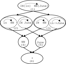
Figure 1: A backing-off lattice for factorization of a dependency event in a bilexical context-free grammar. Each lattice node is denoted by a solid oval and represents a set of events, each of which is represented by a dotted oval. Each lattice edge represents a factorization manner that resolves an event in the parent node (e.g., the left dotted oval in node (3)) into a set of factored events (e.g., the set of events in node (4)).

3 Mixture Model

Through the backing-off lattice, a model is factorized recursively into sub-models. Each node can be applied with more than one factorization manners. We therefore are concerned with the problem of how to approximate the model represented by a lattice node through the models represented by all its children nodes. For instance, how to approximate the distribution of events in node 1 of Figure 1 with factored models represented by nodes 2 and 3. We use a mixture model to interpolates all the factored models. We formulate the mixture model in the following.

Let $\mathcal{E}$ denote a backed-off event (e.g., the Dependency event in the lattice root in figure 1). To get its factored events, we introduce a series of factorization functions: $\Phi_{i},0\leq i\leq I$, each of which corresponds to a lattice edge from $\mathcal{E}$, and factorize $\mathcal{E}$ into a set of sub model events $\mathcal{S}_{i}$, that is,

$$\mathcal{E}\begin{array}[]{c}\Phi_{i}\\ \longrightarrow\\ \\ \end{array}\mathcal{S}_{i}=\{e_{ij}|0\leq j\leq I_{i}\}$$ (4)

where, $e_{ij}$ is the $j$’th sub-event among the set of events obtained by factorizing $\mathcal{E}$ using factorization function $\Phi_{i}$.

We can view $\Phi_{i}$ as a hidden random variable, corresponding to different a factorization manner. It has a prior distribution: $\Pr(\Phi_{i})$, specifying the confidence of selecting the $i$’th path to backoff. We can get,

$$\Pr(\mathcal{S}_{i})=\Pr(\mathcal{E}|\Phi_{i})$$ (5)

The distribution of $\mathcal{E}$ can be derived in the following way,

$$\Pr(\mathcal{E}) = \sum_{\Phi_{i},0\leq i\leq I}\Pr(\mathcal{E},\Phi_{i})$$ (6)

$$= \sum_{\Phi_{i},0\leq i\leq I}\Pr(\Phi_{i})\Pr(\mathcal{E}|\Phi_{i})$$

From Formula 5 and 6, we get

$$\Pr(\mathcal{E})=\sum_{\Phi_{i},0\leq i\leq I}\Pr(\Phi_{i})\Pr(\mathcal{S}_{i})$$ (7)

Formula 7 shows that the probabilistic model governing event $\mathcal{E}$ is approximated by a mixture of its factored models $\Pr(\mathcal{S}_{i})$ using normalized coefficients ($\Pr(\Phi_{i})$). Each coefficient reflects the confidence of selecting a factorization manner.

The sum of $\Phi_{i}$ should be equal to 1. Their values can be handcrafted just for simplicity or trained from held-out data using EM algorithm (A. Dempster, et al., 1977) or other numerical methods such as Powell’s method (W. Press, et al., 1986).

If we assume that the factored events $s_{ij}$ in the value set of a factorization function are independent of each other, we arrive

$$\Pr(\mathcal{E})=\sum_{\Phi_{i},0\leq i\leq I}\Pr(\Phi_{i})\prod_{j}^{|\mathcal{S}_{i}|}\Pr(e_{ij})$$ (8)

Formula 8 shows that if we assume the events in the value set of each projection function are independent of each other, the probability of the value set given factorization function is equal to the multiplication of the probability of each event in the set.

We can derive the mixture model for conditional distributions similarly.

Let us give an example to illustrates the above idea. In the backing-off lattice shown in Figure 1, for the event in node 1 to be factored into event sets in node 2 and 3, respectively, we need to introduce the following factorization functions,

1. $\Phi_{0}$= factorize $\mathcal{E}$ into a lexical dependency and a syntactic dependency.

2. $\Phi_{1}$= factorize $\mathcal{E}$ into sub-events, each of which describes the dependency between (parent or dependent) lexical head and (dependent or parent) nonterminal label.

These functions will project the event into

$$\mathcal{S}_{0}=\{in\rightarrow June,IN\rightarrow NN\}.$$ (9)

$$\mathcal{S}_{1}=\{in\rightarrow NN,IN\rightarrow June\}.$$ (10)

where each of the two sets contains two factored dependency events.

Then based on Formula 7 we get

$$\Pr(IN[in]\rightarrow NN[June])\hskip 56.9055pt$$

$$=\Pr(\Phi_{0})\Pr(in\rightarrow June,IN\rightarrow NN)$$

$$+\Pr(\Phi_{1})\Pr(in\rightarrow NN,IN\rightarrow June)$$ (11)

Assume that factored events in the same set are independent of each other, from Formula 8, we can get

$$\Pr(IN[in]\rightarrow NN[June])\hskip 71.13188pt$$

$$=\Pr(\Phi_{0})\Pr(in\rightarrow June)\Pr(IN\rightarrow NN)$$

$$+\Pr(\Phi_{1})\Pr(in\rightarrow NN)\Pr(IN\rightarrow June)$$ (12)

Now, distribution of $\Pr(IN[in]\rightarrow NN[June])$ is approximated by the mixture of the factored models $\Pr(in\rightarrow June)$, $\Pr(IN\rightarrow NN)$ , $\Pr(in\rightarrow NN)$ and $\Pr(IN\rightarrow June)$ that are obtained based on a pre-defined backing-off lattice.

4 Backing-Off Formula

We have presented a mixture model to approximate a more discriminative model with less discriminative factored models based on a backing-off lattice and a set of factorization functions. A mixture model, however, only combines the factored models obtained by factorizing one lattice node and if we traverse the backing-off lattice, we will get a series of mixtures. We therefore generalize Katz’s backing-off method (Katz, 1987) to organize these mixtures by firing correspondent mixture model when backing-off takes place.

$$\Pr_{bo}(\mathcal{E}_{1}|\mathcal{E}_{2})=\hskip 142.26378pt$$

$$\left\{\begin{array}[]{ll}\frac{C(\mathcal{E}_{1}\mathcal{E}_{2})}{C(\mathcal{E}_{2})}&C(\mathcal{E}_{1}\mathcal{E}_{2})>K\\ \beta_{C(\mathcal{E}_{1}\mathcal{E}_{2})}\frac{C(\mathcal{E}_{1}\mathcal{E}_{2})}{C(\mathcal{E}_{2})}&1\leq C(\mathcal{E}_{1}\mathcal{E}_{2})\leq K\\ \alpha\mathcal{MIXTURE}&otherwise\end{array}\right.$$ (16)

where, $\mathcal{MIXTURE}$ represents the conditional version of the mixture model in Formula 7. $K$ is a frequency threshold for discounting. $\mathcal{E}_{1}$ and $\mathcal{E}_{2}$ refer to, in general, two events that adjacently co-occur in a corpus.

The basic idea of this backing-off method is the same as that of Katz’s. That is, the backing-off formula has a recursive format. At each step of the recursion, there are three branches associated with their firing conditions. If the frequency of the current model event is large enough (such as greater than $K$, Katz used the value of 5 for $K$), the maximum-likelihood estimator (MLE) is used. If the occurrence frequency is within the range of $[1,K]$, the MLE probabilities are discounted in some manner so that some probability mass is reserved for those unseen events. If the model event never occurs in the training data, we use the estimates from the factored model events.

The difference therefore lies in the combination of estimates of factored events. In traditional backing-off methods, there is only one backing-off path to go when the backing-off condition is satisfied. For example, an n-gram only has exactly one (n-1)-gram to be backed-off. However, in our case, we have more than one backing-off paths to go through. None is a branch of another. Then the mixture model obtained in the previous section is embedded here.

$\beta$ are for normalization and can be computed according to (Katz, 1987).

$\alpha$ is also for normalization. It is computed from the amount of reserved probability mass for unseen events. $\alpha$ is a function of $\mathcal{E}_{2}$ because $\mathcal{E}_{2}$ is the given event of a conditional probability, and each conditional probability should satisfy the normalization requirement. It is computed similarly to that in Katz original paper:

$$\alpha = \alpha(\mathcal{E}_{2})$$ (17)

$$= \frac{1-\sum_{\mathcal{E}_{1},\mathcal{E}_{2}:C(\mathcal{E}_{1}\mathcal{E}_{2})>0}\Pr_{bo}(\mathcal{E}_{1}|\mathcal{E}_{2})}{\sum_{\mathcal{E}_{1},\mathcal{E}_{2}:C(\mathcal{E}_{1}\mathcal{E}_{2})=0}\mathcal{MIXTURE}}$$

$$= \frac{1-\sum_{\mathcal{E}_{1},\mathcal{E}_{2}:C(\mathcal{E}_{1}\mathcal{E}_{2})>0}\Pr_{bo}(\mathcal{E}_{1}|\mathcal{E}_{2})}{1-\sum_{\mathcal{E}_{1},\mathcal{E}_{2}:C(\mathcal{E}_{1}\mathcal{E}_{2})>0}\mathcal{MIXTURE}}$$

5 Model Factorizations

Now that we have presented a framework that allows a model event to be factorized along more than paths and combines different paths in a backing-off formula, we now formulate two types of model factorization that are used in natural language modeling. We first introduce some notations.

Let a matrix $\mathcal{M}^{m\times n}$ of random variables represent a linguistic object that simultaneously expresses two types of information in its row and column directions. For example, matrix,

$$\left[\begin{array}[]{ll}nonstop&flights\\ sin&vuelos\end{array}\right]$$ (20)

denotes two lexical dependencies, each of which is the translation the other. It expresses the dependency relationship information in the row direction, and translation relationship information in the column direction.

Let $\mathcal{A}\in\mathcal{M}^{m\times n}$, and $\mathcal{B}$ $\in\mathcal{M}^{m\times n}$, we want to determine $\Pr(\mathcal{A}|\mathcal{B})$ using its factored models. We can either factorize both $\mathcal{A}$ and $\mathcal{B}$ synchronously, or factorize only the conditioning event $\mathcal{B}$, which results in two types of factorizations for different tasks: synchronous factorization, and asynchronous factorization.

5.1 Synchronous factorization

In synchronous factorization, both $\mathcal{A}$ and $\mathcal{B}$ are factorized in the same manner according to some correspondence assumption, and the factored models determines the marginal information of the entire model.

Based on Formula 6 (the mixture model), and the assumption that $\mathcal{A}$ and $\mathcal{B}$ are in sync with with each other on row (or column), we formulate the synchronous factorization as follows:

$$\Pr(\mathcal{A}|\mathcal{B}) = \Pr\left(\Phi_{row}\right)\Pr\left(\mathcal{S}_{row}^{\mathcal{A}}|\mathcal{S}_{row}^{\mathcal{B}}\right)$$ (21)

$$+ \Pr\left(\Phi_{col}\;\;\right)\Pr\left(\mathcal{S}_{col}^{\mathcal{A}}\;|\mathcal{S}_{col}^{\mathcal{B}}\;\right)$$

where,

• $\Phi_{row}$ projects $\mathcal{A}$ and $\mathcal{B}$ on row, respectively, and therefore results in row vectors:

  1. $\mathcal{S}_{row}^{\mathcal{A}}$= $\{(\mathcal{A}_{ij})_{1\times\ n}|1\leq i\leq m\}$

     the set of row vectors of $\mathcal{A}$

  2. $\mathcal{S}_{row}^{\mathcal{B}}$= $\{(\mathcal{B}_{ij})_{1\times n}\;\;|1\leq i\leq m\}$

     the set of row vectors of $\mathcal{B}$

• $\Phi_{col}$ projects $\mathcal{A}$ and $\mathcal{B}$ on column, respectively, and therefore results in column vectors:

  1. $\mathcal{S}_{col}^{\mathcal{A}}\;$= $\{(\mathcal{A}_{ij})_{m\times 1}\;|1\leq j\leq n\}$

     the set of column vectors of $\mathcal{A}$

  2. $\mathcal{S}_{col}^{\mathcal{B}}\;$= $\{(\mathcal{B}_{ij})_{m\times 1}\;\;|1\leq j\leq n\}$

     the set of column vectors of $\mathcal{B}$

Factored models $\Pr\left(\mathcal{S}_{row}^{\mathcal{A}}|\mathcal{S}_{row}^{\mathcal{B}}\right)$ and $\Pr\left(\mathcal{S}_{col}^{\mathcal{A}}|\mathcal{S}_{col}^{\mathcal{B}}\right)$ will be further factorized by other factorization functions, and the results of these factorization functions constitute the backing-off lattice. All these factored models are then combined by the backing-off formula.

Let us give an example. Let

$$\mathcal{A}=\left[\begin{array}[]{l}nonstop\\ sin\end{array}\right]$$ (24)

and let

$$\mathcal{B}=\left[\begin{array}[]{l}flights\\ vuelos\end{array}\right]$$ (27)

Under factorization manner $\Phi_{row}$, and from Formula 21, 24 and 27 we get

$$\Pr\left(\begin{array}[]{c|c}\left[\begin{array}[]{c}nonstop\\ sin\end{array}\right]&\left[\begin{array}[]{c}flights\\ vuelos\end{array}\right]\\ \end{array}\right)$$ (33)

$$= \Pr(\Phi_{row})\Pr\left(\mathcal{S}_{row}^{\mathcal{A}}|\mathcal{S}_{row}^{\mathcal{B}}\right)$$ (34)

where

$$\mathcal{S}_{row}^{\mathcal{A}} = \Phi_{row}(\mathcal{A})=\left\{\left[nonstop\right],\left[sin\right]\right\}$$ (35)

$$\mathcal{S}_{row}^{\mathcal{B}} = \Phi_{row}(\mathcal{B})=\left\{\left[flights\right],\left[vuelos\right]\right\}$$ (36)

and $\Phi_{row}=1$ (normalized).

If we assume that an element in $\mathcal{S}_{row}^{\mathcal{A}}$ is only dependent on the correspondent element in $\mathcal{S}_{row}^{\mathcal{B}}$, we get,

$$\Pr\left(\mathcal{S}_{row}^{\mathcal{A}}|\mathcal{S}_{row}^{\mathcal{B}}\right) = \Pr\left(nonstop|flights\right)$$ (37)

$$\times \Pr\left(sin|vuelos\right)$$

Formula 33 and 37 indicate that, by synchronous factorization, a bilingual lexical dependency model like that in (Alshawi, et al., 2000) is approximated by two factored lexical dependency models , each of which corresponds to one language.

The factorization of a bilexical context-free grammar into a lexical dependency model and a syntactic structure model in (Klein & Manning, 2002) is actually synchronous factorization.

Synchronous factorization is usually used for information combination in the cases that we only have the statistics of those factored models and want to use them to approximate a more complex model; or that we want to simplify a complex model into factored models to gain efficiency (e.g.,  Klein & Manning, 2002).

5.2 Asynchronous factorization

Another type of factorization that is frequently used in statistical language modeling is asynchronous factorization, where only the conditioning event of the conditional probability $\Pr(\mathcal{A}|\mathcal{B})$ is recursively factorized while keeping the conditioned event fixed. The following formula describes the idea.

$$\Pr(\mathcal{A}|\mathcal{B})=\sum_{i=1}^{|\mathcal{B}|}\left(\Pr(\Phi_{i})\Pr(\mathcal{A}|\Phi_{i}(\mathcal{B}))\right)$$ (38)

where $\Phi_{i}$ = “drop the $i$’th element in matrix $\mathcal{B}$”, and $|\mathcal{B}|$ is the number of the elements in matrix $\mathcal{B}$. If we further factorize model $\Pr(\mathcal{A}|\Phi_{i}(\mathcal{B}))$, matrix $\mathcal{B}$ will be a partial matrix that contains a part of elements of the original matrix.

Formula 38 indicates that the original model is recursively factorized into sub-models, and each factorization recursion step has $|\mathcal{B}|$ factorization manners, each of which only drops one element from $\mathcal{B}$.

In the following, we give an example to illustrate the idea of asynchronous factorization. In PP-attachment, suppose we want to factorize model $\Pr(0|is,revenue,from,research)$, which determines the probability of the attachment of preposition phrase “from research” to the noun “revenue” instead of to the verb “is”. Based on Formula 38, we can get,

$$\Pr(1|is,revenue,from,research)=$$

$$\Phi_{revenue}\Pr(1|is,from,research)\hskip 5.69046pt$$

$$+\Phi_{research}\Pr(1|is,revenue,from)\hskip 5.69046pt$$

$$+\Phi_{is}\Pr(1|revenue,from,research)$$ (39)

where $\Phi_{word}$ refers to the factorization function that drops $word$ from the conditioning event of the left hand side model. And the factored models on the right hand side can be further factorized by continuing to traversing the backing-off lattice.

In contrast to that synchronous factorization is used for information combination, asynchronous factorization is usually used for smoothing purpose.

In practice, there might be a compromise between the above two, where we factorize both the conditioned and conditioning events, but not in a synchronous manner. And matrices $\mathcal{A}$ and $\mathcal{B}$ need not to have the same number of rows and columns.

6 Related Works

(Collins & Brooks, 1995) puts forward a method, which actually is asynchronous factorization, for backing-off of models of prepositional phrase attachment, providing a way to mixing the frequencies of different backing off choices at certain recursion step by dividing the sum of frequencies of all the more discriminative model events by those of less discriminative ones if the sum of the frequencies of the less discriminative ones are greater than zero, otherwise, backing-off continues on. One characteristic of this method is that if one of the less discriminative model events has non-zero frequency, the backing-off terminates, no matter whether other events in the same backing-off level are zero or not, whereas the mixture model we introduced to combine parallel backing-off paths is able to to make those zero count event further backoff so that they still can contribute to the final result. And we think this is necessary when we use the backing-off framework for information combination.

It turned out that (Bilmes & Kirchhoff, 2003) were independently working on some similar ideas. They introduced factored models and also generalized the backing-off framework to handle parallel backing-off paths. The differences between their work and ours are (1) Their factored models can actually be categorized into the asynchronous factorization type, where only the conditioning matrix (the feature vector in their paper) is factorized; (2) We also formulated the synchronous factorization type, where both the conditioned and conditioning matrices are factorized synchronously. And we showed that this is useful for combining different information sources; (3) We use a mixture model to combine parallel paths while they selected the the path with the maximum value. We think that combining the contribution of each backing-off path is useful when we want to combine different information resources; (3) In our framework, the result of each factorization function (backing-off path) is a set of events (See Formula 4), not merely one event. And this is usefull when we do the kind of factorization like (Klein & Manning, 2002) using Formula 8.

7 Conclusions

We have presented a framework for language model factorization. We adopt a backing-off lattice to reflect parallel factorizations and to define the paths along which a model is resolved into factored models, we use a mixture model to combine parallel paths in the lattice, and generalize Katz’s backing-off method to integrate all the mixture models got by traversing the entire lattice.

Based on this framework, we formulate two types of model factorizations that are used in natural language modeling.

References

- A. Dempster, et al. (1977) A. Dempster, N. Laird and D. Rubin (1977). “Maximum Likelihood from Incomplete Data via The EM Algorithm,” Journal of Royal Statistical Society, Vol. 39, pp. 1-38, 1977.
- Klein & Manning (2002) D. Klein and C. Manning (2001). “Fast Exact Natural Language Parsing with a Factored Model,” Advances in Neural Information Processing Systems 15 (NIPS-2002), 2002.
- Alshawi, et al. (2000) H. Alshawi, B. Srinivas and S. Douglas (2000). “Learning Dependency Translation Models as Collections of Finite State Head Transducers,” Computational Linguistics, vol. 26, 2000.
- Bilmes & Kirchhoff (2003) J. Bilmes and K. Kirchhoff (2003). “Factored Language Models and Generalized Parallel Backoff,” Human Language Technology Conference, 2003.
- Eisner & Satta (1999) J. Eisner and G. Satta (1999) “Efficient Parsing for Bilexical Context-Free Grammars and Head-Automaton Grammars,” Proceedings of the ACL, 1999.
- Goodman (2001) J. Goodman (2001). “A Bit of Progress in Language Modeling, Extended Version,” Microsoft Research Technical Report MSR-TR-2001-72.
- Collins & Brooks (1995) M. Collins and J. Brooks (1995). “Prepositional Phrase Attachment through a Backed-off Model,” Proceedings of the Third Workshop on Very Large Corpora, 1995.
- Chen & Goodman (1998) S. Chen and J. Goodman (1998). “An Empirical Study of Smoothing Techniques for Language Modeling,” Technical Report TR-10-98, Center for Research in Computing Technology, Harvard University.
- Katz (1987) S. Katz (1987) “Estimation of Probabilities from Sparse Data for the Language Model Component of a Speech Recognizer,” IEEE transactions on Acoustics, Speech, and Signal Processing ASSP-35:400-401.
- W. Press, et al. (1986) W. Press, B. Flannery, S. Teukolsky, and W. Vetterling (1986). “Numerical Recipes, The Art of Scientific Computing,” Cambridge University Press.