Abstract

This article documents the free computer algebra system “gTybalt”. The program is build on top of other packages, among others GiNaC, TeXmacs and Root. It offers the possibility of interactive symbolic calculations within the C++ programming language. Mathematical formulae are visualized using TeX fonts.

PROGRAM SUMMARY

Title of program: gTybalt
Version: 1.0.0
Catalogue number:
Program obtained from: http://www.fis.unipr.it/~stefanw/gtybalt
E-mail: stefanw@fis.unipr.it
License: GNU Public License
Computers: all
Operating system: GNU/Linux
Program language: C++
Memory required to execute: 64 MB recommended
Other programs called: see appendix A
External files needed: none
Keywords: Symbolic calculations, computer algebra.
Nature of the physical problem: Symbolic calculations occur nowadays in all areas of science. gTybalt is a free computer algebra system based on the C++ language.
Method of solution: gTybalt is a “bazaar”-style program, it relies on exisiting, freely-available packages for specific sub-tasks.
Restrictions on complexity of the problem: gTybalt does not try to cover every domain of mathematics. Some desirable algorithms, like symbolic integration are not implemented. It can however easily be extended in new directions. Apart from that, standard restrictions due to the available hardware apply.
Typical running time: Depending on the complexitiy of the problem.

LONG WRITE-UP

1 Introduction

Symbolic calculations, carried out by computer algebra systems, have become an integral part in the daily work of scientists. The advance in algorithms and computer technology has led to remarkable progress in several areas of natural sciences. A striking example is provided by the tremendous progress in the last few years for analytic calculations of so-called loop diagrams in perturbative quantum field theory. It is worth to analyse what the particular requirements on a computer algebra systems for these calculations are: First of all, these tend to be “long” calculations, e.g. the system needs to process large amounts of data and efficiency in performance is a priority. Secondly, the algorithms for the solution of the problem are usually developed and implemented by the physicists themselves. This requires support from the computer algebra system for a programming language which allows to implement complex algorithms for abstract mathematical entities. In other words, it requires support of object oriented programming techniques from the system. On the other hand, these calculations usually do not require that the computer algebra system provides sophisticated tools for all branches of mathematics. Thirdly, despite the fact that these calculations process large amounts of data, the time needed for the implementation of the algorithms usually outweights the actual running time of the program. Therefore convenient development tools are also important. Here I report on the program “gTybalt”, a free computer algebra system. The main features of gTybalt are:

• Object Oriented: gTybalt allows symbolic calculations within the C++ programming language.

• Efficiency for large scale problems: Solutions developed with gTybalt can be compiled with a C++ compiler and executed independently of gTybalt. This is particular important for computer-extensive problems and a major weakness of commercial computer algebra systems.

• Short development cycle: gTybalt can interpret C++ and execute C++ scripts. Solutions can be developed quickly for small-scale problems, either interactively or through scripts, and once debugged, the solutions can be compiled and scaled up to large-scale problems.

• High quality output: Mathematical formulae are visualized using TeX fonts and can easily be converted to LaTeX on a what-you-see-is-what-you-get basis.

gTybalt is a free computer algebra system and distributed under the terms and conditions of the GNU General Public Licence. Compared to other computer algebra systems, it does not try to cover every domain of mathematics. Some desirable algorithms, like symbolic integration are not implemented. However, the modular design of gTybalt allows to incorporate easily new algorithms.

The functionality of a computer algebra system can be divided into different modules, e.g. there will be a module, which displays the output, a second module analysis and interprets the input, a third module does the actual symbolic calculation. Writing a computer algebra system from scratch is a formidable task. Fortunately it is not required, since there are already freely available packages for specific tasks. gTybalt is based on several other packages and provides the necessary communication mechanisms among these packages. gTybalt is therefore a prototype of a “bazaar”-style program [1] and an example of what is possible within the free software community. It should be clearly stated, that without these already existing packages gTybalt would never have been developed and my thanks go to the authors of these packages for sharing their programs with others. In particular gTybalt is build on the following packages:

• The TeXmacs-editor [2] is used to display the output of formulae in high quality mathematical typesetting using TeX fonts.

• gTybalt can also be run from a text window. Then the library eqascii [3] is used to render formulae readable in text mode.

• Any interactive program needs an interpreter for its commands. gTybalt uses the CINT C/C++ interpreter [4], which allows execution of C++ scripts and C++ command line input.

• At the core of any computer algebra system is the module for symbolic and algebraic manipulations. This functionality is provided by the GiNaC-library [5].

• One aspect of computer algebra systems is arbitrary precision arithmetic. Here GiNaC (and therefore gTybalt) relies on the Class Library for Numbers (CLN library) [6].

• Plotting functions is very helpful to quickly visualize results. The graphic abilities of gTybalt are due to the Root-package [7].

• The GNU scientific library is used for Monte Carlo integration [8].

• Optionally gTybalt can be compiled with support for the expansion of transcendental functions. This requires the nestedsums library [9] to be installed.

• Optionally gTybalt can be compiled with support for factorization of polynomials. This requires the NTL library [10] to be installed.

Additional documentation: The manual of gTybalt, which comes with the distribution, provides additional information for this program. Since gTybalt incoporates GiNaC, Root and TeXmacs, you are advised to read also the documentation on GiNaC, Root and TeXmacs. A general introduction to computer algebra can be found in [11] and in the references therein.

This article is organized as follows: The next section gives a brief introduction on how to use the program. Sect. 3 demonstrates for some simple examples how gTybalt can be used for calculations in particle physics. This is the only section which requires some background in particle physics and readers not familiar with this topic may skip this section. Sect. 4 gives details on the design of the program and serves as a guide to the source code. Finally, sect. 5 summarizes this article. In an appendix I give some detailed hints for the installation of the program.

2 Tutorial for gTybalt

This section gives a short tutorial introduction to gTybalt by discussing some small and simple examples.

2.1 Starting gTybalt

gTybalt can be run in the TeXmacs mode or in a simple text mode. To start gTybalt in text mode, type gtybalt. To quit, type quit. To use gTybalt within TeXmacs, first start TeXmacs with the command texmacs. You can then start a gTybalt session by clicking on the terminal symbol and selecting “gTybalt” from the pop-up menu. Alternatively you can start gTybalt from the “Text” menu via “Text $\rightarrow$ Session $\rightarrow$ GTybalt”.

2.2 Command line input

You can type in regular C++ statements which will be processed by CINT. For example

gTybalt> int i=1;
gTybalt> i++;
gTybalt> cout << "The increased number : " << i << endl;
The increased number : 2

The functionality of gTybalt for symbolic and algebraic calculations is provided by the GiNaC-library. The syntax follows the one for the GiNaC-library. For example:

gTybalt> symbol a("a"), b("b");
gTybalt> ex e1=pow(a+b,2);
gTybalt> print(e1);

     2
(b+a)

gTybalt> ex e2=expand(e1);
gTybalt> print(e2);

 2    2
a  + b  + 2 a b

Here print is a gTybalt-subroutine, which prints a variable to the screen. By default, gTybalt does not print anything onto the screen, unless the user specifically asks for a variable to be printed. If gTybalt is running under TeXmacs, the output will be with TeX fonts. There is also a function rawprint which prints the variable e2 as follows:

gTybalt> rawprint(e2);
a^2+b^2+2*a*b

Fig. 1 shows how the output of a further example will look like under TeXmacs.

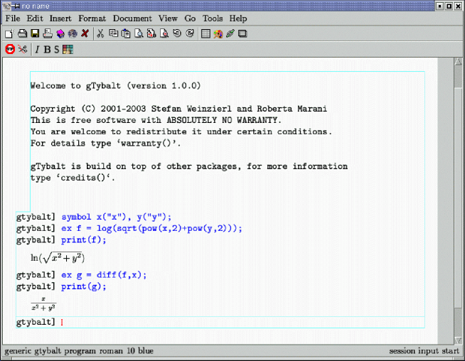
Figure 1: A screenshot for gTybalt when running in TeXmacs mode.

Fig. 2 shows the corresponding output, when gTybalt runs in text mode.

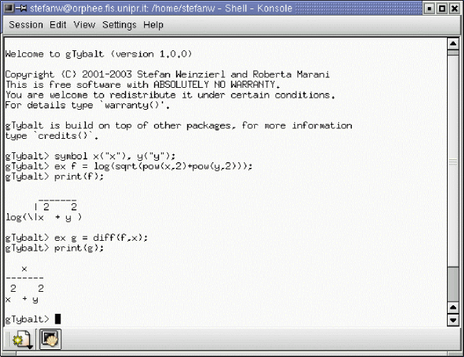
Figure 2: A screenshot for gTybalt when running in text mode.

Within TeXmacs mode there is the possibility to print a session to a postscript file by choosing from the “File” menu the combination “File $\rightarrow$ Export $\rightarrow$ Postscript”. It is also possible to generate for a session a corresponding LaTeX file via “File $\rightarrow$ Export $\rightarrow$ LaTeX”. This is in particular useful if one would like to obtain for a displayed formula the corresponding LaTeX code.

2.3 Scripts

The standard behaviour of the C++/C interpreter CINT is to interpret any command immediately. There is also the possibility to put a few commands into a script and to load this file into a session. This is done through the following commandds:

.L file.C
.x file.C

The .L command loads a script into the session, but does not execute the script. This is useful for a script containing the definition of a function. The .x command loads and executes a script. As an example consider that the file hermite.C contains the following code:

ex HermitePoly(const symbol & x, int n)
{
 ex HKer=exp(-pow(x,2));
 return normal(pow(numeric(-1),n) * diff(HKer,x,n)/HKer);
}

This is just a function which calculates the $n$-th Hermite polynomial. Now try the following lines in gTybalt:

gTybalt> .L hermite.C
gTybalt> symbol z("z");
gTybalt> ex e1=HermitePoly(z,3);
gTybalt> print(e1);

             3
 - 12 z + 8 z

This prints out the third Hermite polynomial. As a further example let the file main.C contain the following code:

{
 symbol z("z");
 for (int i=0;i<5;i++)
  {
   print( HermitePoly(z,i));
  }
}

This is called an “un-named script”. Un-named scripts have to start with an opening “$\{$” and end with a closing “$\}$”. Then the following lines in gTybalt

gTybalt> .L hermite.C
gTybalt> .x main.C

will print the first five Hermite polynomials.

2.4 Plots

A function can be plotted as follows:

gTybalt> symbol x("x");
gTybalt> ex f1=sin(x);
gTybalt> plot(f1,x,0,20);

This will plot $\sin(x)$ in the intervall from 0 to 20.

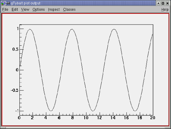
Figure 3: The plot for the function $\sin(x)$ for $x$ from $0$ to $20$.

To clear the window with the plot, choose from the menubar of the plot “File $\rightarrow$ Quit ROOT”.
Similar, a scalar function of two variables can be plotted as follows:

gTybalt> symbol x("x"), y("y");
gTybalt> ex f2=sin(x)*sin(y);
gTybalt> plot(f2,x,y,0,10,0,20);

This will plot $\sin(x)\sin(y)$ for $x$ from $0$ to $10$ and $y$ from $0$ to $20$. Fig. 4 shows the output from the plotting routine.

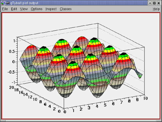
Figure 4: The plot for the function $\sin(x)\sin(y)$ for $x$ from $0$ to $10$ and $y$ from $0$ to $20$.

To view the plot from a different angle, just grap the plot with the mouse and move it around. There is a wide variety of options on how to draw a graph. To access the draw panel, click on the right mouse button, when the mouse is placed inside the window containing the plot and choose “DrawPanel” from the pop-up menu. The options include among others lego- and contour-plots. The default option corresponds to the style “surf” and draws a (coloured) surface.
The plot can be saved to a file. For example, to save the plot as a postscript file, choose from the “File” menu the option “Save As canvas.ps”.

2.5 Numerical integration

Functions can be integrated numerically by Monte Carlo integration. For example to evaluate the integral

$$\int\limits_{0}^{1}dx\int\limits_{0}^{1}dy\int\limits_{0}^{1}dz\;xyz$$ (1)

one types

gTybalt> symbol x("x"), y("y"), z("z");
gTybalt> ex f = x*y*z;
gTybalt> ex g = intnum(f,lst(x,y,z),lst(0,0,0),lst(1,1,1));
gTybalt> print(g);
0.12500320720479463077

The result of the integration can also be accessed with the help of the global variable
gTybalt_int_res. In addition the global variables gTybalt_int_err and
gTybalt_int_chi2 give information on the error and the $\chi^{2}$. For our example, one gets

gTybalt> print(gTybalt_int_res);
0.125003
gTybalt> print(gTybalt_int_err);
5.26234e-06
gTybalt> print(gTybalt_int_chi2);
0.385639

The Monte Carlo integration uses the adaptive algorithm VEGAS [12]. gTybalt uses the implementation from the GNU Scientific Library. The algorithm first uses gTybalt_int_iter_low iterations with gTybalt_int_calls_low calls to obtain some rough information where the integrand is largest in magnitude. The results of this run are discarded, but the grid is kept. The algorithm then performs gTybalt_int_iter_high iterations with gTybalt_int_calls_high calls to obtain a Monte Carlo estimate. The default values are

gTybalt> print(gTybalt_int_iter_low);
5
gTybalt> print(gTybalt_int_calls_low);
10000
gTybalt> print(gTybalt_int_iter_high);
10
gTybalt> print(gTybalt_int_calls_low);
100000

The values of these variables can be adjusted by the user. For functions of one or two variables there are in addition the following simpler forms

double intnum(ex expr, ex x, double xmin, double xmax);
double intnum(ex expr, ex x, ex y, double xmin, double xmax,
                                   double ymin, double ymax);

2.6 Factorization

When gTybalt is compiled with the NTL library, gTybalt provides an interface to factorize univariate polynomials with integer coefficients. For example

gTybalt> symbol x("x");
gTybalt> ex f = expand( pow(x+2,13)*pow(x+3,5)*pow(x+5,7)*pow(x+7,2) );
gTybalt> ex g = factorpoly(f,x);
gTybalt> print(g);

        2        5        7        13
 (7 + x)  (3 + x)  (5 + x)  (2 + x)

If the first argument of the function factorpoly is not an univariate polynomial with integer coefficients, it returns unevaluated.

2.7 Expansion of transcendental functions

When gTybalt is compiled with the nestedsums library, gTybalt provides an interface to expand a certain class of transcendental functions in a small parameter. The class of functions comprises among others generalized hypergeometric functions, the first and second Appell function and the first Kampe de Feriet function. A hypergeometric function can be expanded as follows:

gTybalt> symbol x("x"), eps("epsilon");
gTybalt> transcendental_fct_type_A F21(x,lst(1,-eps),lst(1-eps),lst(1-eps),
         lst(1,-eps));
gTybalt> ex f = F21.set_expansion(eps,5);
gTybalt> rawprint(f);
-Li(3,x)*epsilon^3-Li(2,x)*epsilon^2-Li(4,x)*epsilon^4-Li(1,x)*epsilon
+Z(Infinity)

This expands the hypergeometric function ${}_{2}F_{1}(1,-\varepsilon;1-\varepsilon;x)$ in $\varepsilon$ up to order 5 and agrees with the known expansion

$${}_{2}F_{1}(1,-\varepsilon;1-\varepsilon;x) = 1-\varepsilon\;\mbox{Li}_{1}(x)-\varepsilon^{2}\;\mbox{Li}_{2}(x)-\varepsilon^{3}\;\mbox{Li}_{3}(x)-\varepsilon^{4}\;\mbox{Li}_{4}(x)+{\cal O}(\varepsilon^{5}).$$ (2)

The algorithm for the expansion is based on an algebra for nested sums [13]. Z(Infinity) represent the unit element in this algebra and is equal to 1.

3 Examples from particle physics

In this section I discuss some examples from particle physics. The reader not familiar with this field may skip this section. As before, all examples will be very elementary.

3.1 Calculation of Born matrix elements

Here I discuss how to calculate the Born matrix element for the process $\gamma^{\ast}\rightarrow qg\bar{q}$. There are only two contributing Feynman diagrams, which are shown in fig. 5.

Figure 5: The Feynman diagrams contributing to the process $\gamma^{\ast}\rightarrow qg\bar{q}$.

The following script calculates the Born matrix element squared:

{
// this script calculates the Born matrix element squared for
// photon -> quark gluon antiquark
// trivial coupling and colour prefactors are ignored

ex onehalf = numeric(1,2);
ex D       = numeric(4);

// indices
varidx mu(symbol("mu"),D), nu(symbol("nu"),D);
varidx rho(symbol("rho"),D), sigma(symbol("sigma"),D);

// symbols for fourvectors
symbol p1("p1","p_1"), p2("p2","p_2"), p3("p3","p_3");
symbol p12("p12","p_{12}"), p23("p23","p_{23}");

// symbols for scalarproducts
symbol s12("s12","s_{12}"), s23("s23","s_{23}"), s13("s13","s_{13}");
symbol s123("s123","s_{123}");

// siderelations for simplifications
lst l_mom  = lst( p12==p1+p2, p23==p2+p3 );
lst l_sinv = lst( s13==s123-s12-s23 );

// table for scalarproducts
scalar_products sp;
sp.add(p1,p1,0);
sp.add(p2,p2,0);
sp.add(p3,p3,0);
sp.add(p1,p2,onehalf*s12);
sp.add(p1,p3,onehalf*s13);
sp.add(p2,p3,onehalf*s23);

// polarization sums
ex q_pol_sum      = dirac_slash(p1,D,1);
ex qbar_pol_sum   = dirac_slash(p3,D,1);
ex gluon_pol_sum  = -lorentz_g(rho,sigma);
ex photon_pol_sum = -lorentz_g(mu,nu);

// Feynman diagrams
ex amplitude = (-I) * dirac_gamma(rho.toggle_variance(),1)
     * I / s12 * dirac_slash(p12,D,1)
     * (-I) * dirac_gamma(mu.toggle_variance(),1)
   +
     (-I) * dirac_gamma(mu.toggle_variance(),1)
     * I / s23 * dirac_slash(-p23,D,1)
     * (-I) * dirac_gamma(rho.toggle_variance(),1);

ex amplitude_conj = I * dirac_gamma(nu.toggle_variance(),1)
     * (-I) / s12 * dirac_slash(p12,D,1)
     * I * dirac_gamma(sigma.toggle_variance(),1)
   +
     I * dirac_gamma(sigma.toggle_variance(),1)
     * (-I) / s23 * dirac_slash(-p23,D,1)
     * I * dirac_gamma(nu.toggle_variance(),1);

// matrix element squared
ex M3_raw = amplitude * qbar_pol_sum * amplitude_conj * q_pol_sum
           * gluon_pol_sum * photon_pol_sum;

// substitute and expand
ex M3_temp = M3_raw.subs(l_mom).expand(expand_options::expand_indexed);

// take trace and simplify
ex M3 = dirac_trace(M3_temp,1).simplify_indexed(sp).subs(l_sinv).expand();
}

Running this script in gTybalt will yield

$$M_{3} = 16\frac{s_{123}^{2}}{s_{12}s_{23}}-16\frac{s_{123}}{s_{12}}+8\frac{s_{23}}{s_{12}}-16\frac{s_{123}}{s_{23}}+8\frac{s_{12}}{s_{23}},$$ (3)

which is the correct result. The advantage of an interactive program in the debugging phase is, that one has access to intermediate variables (like “M3_raw” or “M3_temp”), which can be printed in a human-readable form. Once debugged, the file (with minor modifications) can be compiled and linked against the GiNaC-library. It can then be executed without invoking gTybalt.

3.2 Integration over phase space

The result from the previous subsection can be writen as

$$M_{3} = F\left(\frac{s_{12}}{s_{123}},\frac{s_{13}}{s_{13}+s_{23}}\right)+F\left(\frac{s_{23}}{s_{123}},\frac{s_{13}}{s_{12}+s_{13}}\right),$$ (4)

where

$$F(y,z) = \frac{8}{y}\left[\frac{2}{1-z(1-y)}-2+(1-y)(1-z)\right].$$ (5)

Integrated over the appropriate phase space, this expression gives a higher order contribution to the process $\gamma^{\ast}\rightarrow q\bar{q}$. The appropriate phase space measure in terms of the $y$ and $z$ variables reads

$$d\phi_{3} = \frac{s_{123}}{128\pi^{3}}\int\limits_{0}^{1}dy\;(1-y)\int\limits_{0}^{1}dz.$$ (6)

This integral diverges for $y=0$ and a standard procedure (“phase space slicing”) splits the integral into two regions, the interval $[0,y_{min}]$ and the intervall $[y_{min},1]$. In the first region the integral is treated analytically in $D$ dimensions and combined with virtual loop corrections such that the infrared divergences cancel in the sum. This will not be discussed here further. The second region gives a finite contribution, which depends on the parameter $y_{min}$ and is treated numerically. One is therefore interested in evaluating integrals of the following type:

$$\int\limits_{y_{min}}^{1}dy\;(1-y)\int\limits_{0}^{1}dz\;F(y,z)$$ (7)

The following script “phasespace.C” will perform this integration numerically:

{
symbol y("y"), z("z");
double ymin = 0.01;

ex integrand = (1-y) * 8/y * (2/(1-z*(1-y))-2+(1-y)*(1-z));
ex result = intnum(integrand,y,z,ymin,1,0,1);
}

One obtains:

gTybalt> .x phasespace.C
gTybalt> print(gTybalt_int_res);
124.322
gTybalt> print(gTybalt_int_err);
0.00168332

For this simple example the exact result can be calculated, which for $y_{min}=0.01$ is approximately $124.318$.

3.3 Loop integrals

Loop integrals occur in higher orders in perturbation theory. An example for a loop integral is given by the following three-point function

$$I = \frac{\Gamma(1-2\varepsilon)}{\Gamma(1+\varepsilon)\Gamma(1-\varepsilon)^{2}}\left(-s_{123}\right)^{\nu_{123}-m+\varepsilon}\int\frac{d^{D}k_{1}}{i\pi^{D/2}}\frac{1}{(-k_{1}^{2})^{\nu_{1}}}\frac{1}{(-k_{2}^{2})^{\nu_{2}}}\frac{1}{(-k_{3}^{2})^{\nu_{3}}},$$ (8)

where $k_{1}=k_{2}+p_{1}+p_{2}$, $k_{2}=k_{3}+p_{3}$, $D=2m-2\varepsilon$, $s_{123}=(p_{1}+p_{2}+p_{3})^{2}$, $\nu_{123}=\nu_{1}+\nu_{2}+\nu_{3}$ and $p_{1}^{2}=p_{2}^{2}=p_{3}^{2}=0$.

Figure 6: A one-loop integral with two external off-shell legs.

A diagram for this integral is shown in fig. 6. It is not too complicated to show that this integral evaluates to the following hypergeometric function

$$I = \frac{\Gamma(1-2\varepsilon)}{\Gamma(1+\varepsilon)\Gamma(1-\varepsilon)^{2}}\frac{1}{\Gamma(\nu_{1})\Gamma(\nu_{2})}\frac{\Gamma(m-\varepsilon-\nu_{1})\Gamma(m-\varepsilon-\nu_{23})}{\Gamma(2m-2\varepsilon-\nu_{123})}$$ (9)

$$\times\sum\limits_{n=0}^{\infty}\frac{\Gamma(n+\nu_{2})\Gamma(n-m+\varepsilon+\nu_{123})}{\Gamma(n+1)\Gamma(n+\nu_{23})}\left(1-x\right)^{n},$$

where $x=s_{12}/s_{123}$. The task is now to expand this expression for specific integer values of $\nu_{1}$, $\nu_{2}$, $\nu_{3}$ and $m$ in the small parameter $\varepsilon$. With the help of the nestedsums library this can be done as follows:

{
symbol x("x"), eps("epsilon");
ex nu1 = 1;
ex nu2 = 1;
ex nu3 = 1;
ex m   = 2;

ex nu23  = nu2+nu3;
ex nu123 = nu1+nu2+nu3;

transcendental_fct_type_A F21(1-x,lst(nu2,nu123-m+eps),lst(nu23),
        lst(1-2*eps,m-eps-nu1,m-eps-nu23),
        lst(1+eps,1-eps,1-eps,nu1,nu2,2*m-2*eps-nu123));
ex result = F21.set_expansion(eps,1);
}

This script calculates the expansion for $\nu_{1}=\nu_{2}=\nu_{3}=1$ and $m=2$ to order $\varepsilon^{0}$ and one obtains

$$\frac{\mbox{Li}_{1}(1-x)}{\varepsilon(-1+x)}+\frac{S_{0,2}(1-x)}{-1+x}+{\cal O}(\varepsilon).$$ (10)

Expressing the Nielsen polylog $S_{0,2}(1-x)$ in terms of standard logarithms this is equal to

$$\frac{\ln x}{\varepsilon(1-x)}-\frac{\ln^{2}x}{2(1-x)}+{\cal O}(\varepsilon)$$ (11)

and is the correct result.

4 Design of the program

This section gives some technical details on the design of the program and serves as a guide to the source code. The reader who is primarily interested in using the program just as an application may skip this section in a first reading. After a general overview of the system I discuss two technical points concerning threads and dynamic loading, where a few explanations might be useful to understand the source code.

4.1 Structural overview

A structural overview for gTybalt is shown in fig. 7.

Figure 7: Structural overview for gTybalt.

gTybalt consists of three parts, labelled gTybalt-bin, gTybalt-dictionary and gTybalt-lib, which ensure communication between the different modules on which gTybalt is based. The first part, gTybalt-bin is either called from TeXmacs (in TeXmacs-mode) or directly from the shell (when issuing the command “gtybalt” from a shell) and implements an event loop. This program reads input from the keyboard, sends the commands to the C++ interpreter CINT for execution and directs the output either to TeXmacs or to a text window.
The program CINT interprets the commands. For this purpose it uses a library called
gTybalt-dictionary, which can be thought of as a look-up table where to find the actual implementations of the encountered function calls. The source code for this library is generated automatically during the build phase of gTybalt. A file “LinkDef.h” specifies which functions and classes to include into this library. The library is then generated from the header files for these functions and classes. The CINT interpreter is not $100\%$ standard C++ compatible and there are certain constructs, which cannot be processed by CINT. Therefore the header files for the GiNaC-library are first copied to a temporary directory and then processed by a perl script, which comments out any parts which cannot be fed into CINT.
Finally, the library gTybalt-lib is an ordinary library, defining gTybalt-specific functions like print, factorpoly or intnum. It depends in turn on other libraries, like Eqascii, GSL or NTL, which are however not visible in the interactive interface.

4.2 Threads and the plotting routine

When plotting a function, it is desirable to have the window with the plot appearing on the screen, but at the same time still be able to work in the main window of gTybalt. Since there are now two possible actions which the user can take (e.g. typing new commands in the main window and modifying the plot inside the window with the plot) this is implemented using different threads. When starting gTybalt, the program will create a separate thread, which waits on a condition that a function should be plotted. When a plotting command is issued, CINT invokes a function, which just prepares some variables for the plot, signals that there is something to be plotted and then returns. Therefore after the return of this function the user can issue new commands in the main window of gTybalt. The thread waiting on the condition for plotting a function will wake up, plot the function and provide an event handler for events concerning the window with the plot. Therefore the user can now take actions in both the main window for gTybalt and the window with the plot. Once the window with the plot is cleared (by choosing from the menubar of the plot “File $\rightarrow$ Quit ROOT”) the thread for plots will fall into sleep again and wait till another plotting command is issued. Thread safety is guarenteed by copying the relevant expressions for the function to be plotted to global variables and by the reference counting mechanism of GiNaC: The expression to be plotted will be pointed at by at least one (global) variable, therefore it will not be modified. While a plot is displayed on the screen, any command to plot another function will be ignored. The user must first clear the window with the plot.

4.3 Dynamic loading of modules and numerical integration

The default behaviour for numerical evaluation of a function uses the arbitrary precision arithmetic provided by the CLN library. For Monte Carlo integration, where a function needs to be evaluated many times, this is quite slow and therefore inefficient. It is also not needed, since statistical errors and not rounding errors tend to dominate the error of the final result. Therefore a different approach has been implemented for the numerical Monte Carlo integration: The function to be integrated is first written as C code to a file, this file is then compiled with a standard C compiler and the resulting executable is loaded dynamically (e.g. as a “plug-in”) into the memory space of gTybalt and the Monte Carlo integration routine uses this compiled C function for the evaluations.

5 Summary

In this article I discussed the free computer algebra system “gTybalt”. It has a modular structure and is based on other, freely available packages. gTybalt offers the possibility of interactive symbolic calculations within the C++ programming language. Mathematical formulae are visualized using TeX fonts. It can be extended easily by adding new libraries to it.

Acknowledgements

The program described here relies on other programs. I would like to thank the authors of these packages: Ch. Bauer, A. Frink, R. Kreckel, J. van der Hoeven, M. Goto, R. Brun, F. Rademakers, B. Haible, P. Borys, V. Shoup, M. Galassi, J. Davies, J. Theiler, B. Gough, G. Jungman, M. Booth and F. Rossi.

Appendix A Installation

A.1 Prerequisities

gTybalt uses TeXmacs, Root, GiNaC and the GNU scientific library. These packages are needed before one starts to build gTybalt. TeXmacs depends on LaTeX and Guile Scheme, GiNaC on the CLN library. One therefore needs also these packages. The C++/C interpreter CINT is not needed as a separate package, since it is already included in Root.

Building gTybalt requires a ANSI-compliant C++-compiler. It is strongly recommended to use gcc. The version number of the gcc compiler can be obtained by

$ gcc -v

It is recommended to use version gcc 2.95.3. There have been problems reported with versions 2.96 and 3.x.

gTybalt 1.0.0 works with

 gcc 2.95.3,
 GiNaC 1.0.14,
 Root 3.03.09,
 TeXmacs 1.0.1,
 GSL 1.2,
 CLN 1.1.5,
 NTL 5.0c,
 nestedsums 1.1.1.

gTybalt has been tested with these versions and you are advised to use EXACTLY those.
You can follow the steps below to build all relevant packages in the right order.
You need LaTeX to be installed. You can check whether the LaTeX binaries exist in your path by

$ which latex

Usually LaTeX is already included in a standard Linux distribution.
You further need Guile Scheme to be installed. You can check by

$ which guile

If Guile is not installed, you can download it from

 http://www.gnu.org/software/guile

and follow the installation instructions.
Installation of TeXmacs: Having LaTeX and Guile Scheme installed, you can build and install TeXmacs. TeXmacs can be obtained from

 http://www.texmacs.org

Follow the installations instructions there.
Installation of Root: The Root package can be obtained from

 ftp://root.cern.ch/root

Follow the installation instructions there. Note that the configuration command has a slightly different syntax as compared to the standard autotools configuration script. Further note that the Root package includes also the C++/C interpreter CINT.
Installation of the CLN library: GiNaC requires the CLN library, available from either one of the following FTP-sites:

 ftp://ftp.santafe.edu/pub/gnu/
 ftp://ftp.ilog.fr/pub/Users/haible/gnu/
 ftp://ftpthep.physik.uni-mainz.de/pub/gnu/

Follow the installation instructions in the manual.
Installation of GiNaC: You find GiNaC at

 http://www.ginac.de

Unpack the GiNaC source code and follow the installation instructions of GiNaC. There is no need to build the package ginac-cint, gTybalt uses the CINT implementation of Root and builds the necessary dictionary later.
Installation of the GNU scientific library: You find the GNU scientific library at

 http://sources.redhat.com/gsl

Unpack the source code and follow the installation instructions of the GNU scientific library.
Optionally gTybalt can be compiled with support for factorization of polynomials. In this case, the NTL library has to be installed. The NTL library is available from

 http://www.shoup.net/ntl

Configure the NTL library with the option "NTL_STD_CXX=on". This puts the classes of the NTL library into a namespace "NTL". This option is needed by gTybalt.
Optionally gTybalt can be compiled with support for the expansion of transcendental functions. In this case, the nestedsums library has to be installed. The nestedsums library is available from

 http://www.fis.unipr.it/~stefanw/nestedsums

Follow the installations instructions there.

A.2 Building gTybalt

As with any autoconfiguring GNU software, installation proceeds through the following steps:

$ ./configure
$ make
[become root if necessary]
$ make install

The "configure" script can be given a number of options to enable and disable various features. For a complete list, type:

$ ./configure --help

A few of the more important ones:

• --prefix=PREFIX: install architecture-independent files in PREFIX [defaults to
  /usr/local]

• --exec-prefix=EPREFIX: install architecture-dependent files in EPREFIX [defaults to the value given to --prefix]

• --with-nestedsums: If the nestedsums library is installed, one may give this option to enable support for the expansion of transcendental functions.

• --with-ntl: If the NTL library is installed, one may give this option to enable support for the factorization of polynomials.

• --with-ntl-prefix=PREFIX: If the NTL library is installed in an unusual location, the value of PREFIX informs the configure script where to find the NTL library.

• --with-gmp-prefix=PREFIX: The NTL library can be compiled with the GMP library (GNU Multiple Precision Arithmetic Library) [14]. If the GMP library is installed in an unusual location, the value of PREFIX informs the configure script where to find the GMP library.

If you install the executables and the libraries in non-standard directories, you have to set the PATH and the LD_LIBRARY_PATH variables correspondingly.

A.3 Example of a complete installation

Here is an example of a complete installation. We assume that LaTeX is already installed and that a suitable compiler exists. We further assume that we do not have root privileges, therefore we have to install the programs in an unusual directory, which we take to be
/home/username/local. We further decide to build only shared libraries (where this is possible) and we would like to set up gTybalt with support for factorization and for the expansion of transcendental functions. This requires to install the NTL library and the nestedsums library. We decide to build the NTL library in conjunction with the GMP (GNU Multi-Precision library) for enhanced performance. Furthermore we assume that we have unpacked all relevant source packages into separate directories. The commands to build a specific package are entered from the top-level directory of the specific package. For concreteness we assume that we have a Linux PC with a Bourne compatible shell.
We start with Guile:

$ ./configure --prefix=/home/username/local
$ make
$ make install

We then set the environment variables (probably in a file like .bash_profile):

export GUILE_LOAD_PATH=/home/username/local
export PATH=/home/username/local/bin:$PATH
export LD_LIBRARY_PATH=/home/username/local/lib:$LD_LIBRARY_PATH

Building TeXmacs is done in a similar way

$ ./configure --prefix=/home/username/local
$ make
$ make install

In the next step we build the Root package (note the slightly different syntax):

$ ./configure linux --prefix=/home/username/local
  --etcdir=/home/username/local/etc
$ gmake
$ gmake install

and we set the variable ROOTSYS (probably in a file like .bash_profile):

export ROOTSYS=/home/username/local

The GMP library is build as follows:

$ ./configure --prefix=/home/username/local
$ make
$ make install

To build the NTL library we issue the commands:

$ cd src
$ ./configure PREFIX=/home/username/local NTL_STD_CXX=on
  NTL_GMP_LIP=on GMP_PREFIX=/home/username/local
$ make
$ make install

Note the slight modified form how the arguments are passed to the configure script.
To build the CLN-library:

$ ./configure --prefix=/home/username/local --enable-static=no
$ make
$ make install

To build GiNaC:

$ ./configure --prefix=/home/username/local --enable-static=no
$ make
$ make install

To build the GNU scientific library:

$ ./configure --prefix=/home/username/local --enable-static=no
$ make
$ make install

To build the nestedsums library:

$ ./configure --prefix=/home/username/local --enable-static=no
$ make
$ make install

And finally we build gTybalt:

$ ./configure --prefix=/home/username/local --enable-static=no
  --with-nestedsums --with-ntl
  --with-ntl-prefix=/home/username/local
  --with-gmp-prefix=/home/username/local
$ make
$ make install

This completes the installation procedure.

References

- [1] E. Raymond, “The Cathedral and the Bazaar”, http://catb.org/~esr/writings/cathedral-bazaar.
-
[2]
J. van der Hoeven,
Cahiers GUTenberg 39-40, 39 (2001);
J. van der Hoeven, “TeXmacs” (1999), http://www.texmacs.org. - [3] P. Borys, “eqascii” (2001), http://dione.ids.pl/~pborys/software/linux.
-
[4]
M. Goto,
“C++ Interpreter - CINT”, CQ publishing, ISBN 4-789-3085-3 (in japanese);
M. Goto, “CINT”, http://root.cern.ch/root/Cint.html. -
[5]
C. Bauer, A. Frink, and R. Kreckel,
J. Symbolic Computation 33, 1 (2002), cs.sc/0004015;
“GiNaC library”, http://www.ginac.de. - [6] B. Haible, “CLN library” (1999), http://www.ginac.de/CLN.
-
[7]
R. Brun and F. Rademakers,
Nucl. Inst. & Meth. in Phys. Res. A389, 81 (1997);
“Root”, http://root.cern.ch. - [8] M. Galassi et al., “GNU scientific library”, http://sources.redhat.com/gsl.
- [9] S. Weinzierl, Comput. Phys. Commun. 145, 357 (2002), math-ph/0201011; “nestedsums library”, http://fis.unipr.it/~stefanw/nestedsums.
- [10] V. Shoup, “NTL library” (1990), http://www.shoup.net.
- [11] S. Weinzierl, “Computer algebra in particle physics” (2002), hep-ph/0209234.
-
[12]
G. P. Lepage,
J. Comput. Phys. 27, 192 (1978);
G. P. Lepage, “VEGAS: an adaptive multidimensional integration program”, CLNS-80/447. - [13] S. Moch, P. Uwer, and S. Weinzierl, J. Math. Phys. 43, 3363 (2002), hep-ph/0110083.
- [14] T. Granlund and K. Ryde, “GNU Multiple Precision Arithmetic Library”, http://www.swox.com/gmp.