TCTL Inevitability Analysis of Dense-time Systems

Abstract

Inevitability properties in branching temporal logics are of the syntax $\forall\Diamond\phi$, where $\phi$ is an arbitrary (timed) CTL formula. In the sense that ”good things will happen”, they are parallel to the ”liveness” properties in linear temporal logics. Such inevitability properties in dense-time logics can be analyzed with greatest fixpoint calculation. We present algorithms to model-check inevitability properties both with and without requirement of non-Zeno computations. We discuss a technique for early decision on greatest fixpoints in the temporal logics. Our algorithms come with a $d$-parameter for the measurement of time-progress. We have experimented with various issues, which may affect the performance of TCTL inevitability analysis. Specifically, we report the performance of our implementation w.r.t. various $d$-parameter values and with or without the non-Zeno computation requirement in the evaluation of greatest fixpoints. We have also experimented with safe abstration techniques for model-checking TCTL inevitability properties. Analysis on the experiment data helps clarify how various techniques can be used to improve verification of inevitability properties.

Keywords: branching temporal logics, TCTL, real-time systems, inevitability, model-checking, greatest fixpoint, abstraction

1 Introduction

In the research of verification, very often two types of specification properties attract most interest from academia and industry. The first type specifies that ”bad things will never happen” while the second type specifies that ”good things will happen”[3]. In linear temporal logics, the former is captured by modal operator $\Box$ while the latter by $\Diamond$[29]. Tremendous research effort has been devoted to the efficient analysis of these two types of properties in the framework of linear temporal logics[25]. In the branching temporal logics of (timed) CTL[1, 11, 12], these two types can be mapped to modal operators $\forall\Box$ and $\forall\Diamond$ respectively. $\forall\Box$ properties are called safety properties while $\forall\Diamond$’s are usually called inevitability properties[16, 27]. In the domain of dense-time system verification, people have focused on the efficient analysis of safety properties[15, 19, 23, 24, 28, 33, 34, 35, 36, 37, 40]. Inevitability properties in Timed CTL (TCTL)[1, 17] are comparatively more complex to analyze due to the following reason. In the framework of model-checking, to analyze an inevitability property, say $\forall\Diamond\phi$, we actually compute the set of states that satisfy the negation of inevitability, in symbols $[[\exists\Box\neg\phi]]$, and then use the intersection emptiness between $[[\exists\Box\neg\phi]]$ and the initial states for the answer to the inevitability anlaysis. However, property $\exists\Box\neg\phi$ in TCTL semantics is only satisfied with non-Zeno computations[1]. (Zeno computations are those counter-intuitive infinite computations whose execution times converge to a finite value[17].) For example, a specification like

”along all computations, eventually a bus collision will happen in three time units”

can be violated by a Zeno computation whose execution time converges to a finite timepoint, e.g. 2.9. Such requirement on non-Zeno computations may add complexity to the evaluation of inevitability properties. In this work, we present our symbolic TCTL model-checking algorithm which can handle the non-Zeno requirement in the evaluation of greatest fixpoints. The evaluation of inevitability properties in TCTL involves nested reachability analysis and demands much higher complexity than simple safety analysis.

To contain the complexity of TCTL inevitability, it is important to integrate new and old techniques for a performance solution. In this paper, we investigate three approaches. In the first approach, we investigate how to adjust a parameter value in our greatest fixpoint evaluation algorithms for better performance. We have carried out experiments to get insight on this issue.

In the second approach, we present a technique called Early Decision on the Greatest Fixpoint (EDGF). The idea is that, in the evaluation of the greatest fixpoints, we start with a state-space and iteratively pare states from it until we reach a fixpoint. Throughout iterations of the greatest fixpoint evaluations, the state-space is non-increasing. Thus, if in a middle greatest fixpoint evaluation iteration, we find that target states have already been pared from the greatest fixpoint, we can conclude that it is not possible to include these target states in the fixpoint. Through this technique, we can reduce time-complexity irrelevant to the answer of the model-checking. As reported in section 9, significant performance improvement has been observed in several benchmarks.

Our third approach is to use abstraction techniques[9, 10, 39]. We shall focus on a special subclass, TCTL^∀, of TCTL in which every formula can be analyzed with safe abstraction if over-approximation is used in the evaluation of its negation. For example, we may write the following formula in the subclass.

$\forall\Box\left(\mbox{\tt request}\rightarrow\forall\Box\left(\mbox{\tt service}\rightarrow\forall\Diamond{\tt request}\right)\right)$

This formula says that if a request is responded by a service, then a request will follow the service. This subclass allows for nested modal formulas and we feel that it captures many TCTL inevitability properties.

One challenge in designing safe abstraction techniques in model-checking is making them accurate enough to discern many true properties, while still allowing us to enhance verification performance. In previous research, people have designed many abstraction techniques for reachability analysis[4, 15, 28, 39, 40], as have we[38]. However, for model-checking formulas in TCTL^∀, abstraction accuracy can be a bigger issue since the inaccuracy in abstraction can be potentially magnified when we use inaccurate evaluation results of nested modal subformulas to evaluate nesting modal subformulas with abstraction techniques. Thus it is important to discern accuracy of previous abstraction techniques in discerning true TCTL^∀formulas.

In this paper, we also discuss another possibility for abstract evaluation of greatest fixpoints, which is to omit the requirement for non-Zeno computations in TCTL semantics. As reported in section 9, many benchmarks are true even without exclusion of Zeno computations.

Finally, we have implemented these ideas in our model-checker/simulator red 4.1[35]. We report here our experiments to observe the effects of parameter values, EDGF, various abstraction techniques, and non-Zeno requirements on our inevitability analysis. We also compare our analysis with Kronos 5.1[15, 40], which is another model-checker for full TCTL.

Our presentation is ordered as follows. Section 2 discusses several related works. Sections 3 and 4 give brief presentations of our model, timed automata (TA), and TCTL. Section 5 presents our TCTL model-checking algorithm with requirements for non-Zeno computations. Section 6 improves our model-checking algorithm using an EDGF technique. Section 7 gives another version of a greatest fixpoint evaluation algorithm by omitting the requirement of non-Zeno computations. Section 8 identifies the subclass TCTL^∀of TCTL which supersedes many inevitability properties, while allowing for safe abstract model-checking by using over-approximation techniques. Section 9 illustrates our experiment results and helps clarify how various techniques can be used to improve analysis of inevitability properties. Section 10 is the conclusion.

2 Related work

The TA model with dense-time clocks was first presented in [2]. Notably, the data-structure of DBM is proposed in [14] for the representation of convex state-spaces of TA. The theory and algorithm of TCTL model-checking were first given in [1]. The algorithm is based on region graphs and helps manifest the PSPACE-complexity of the TCTL model-checking problem.

In [17], Henzinger et al proposed an efficient symbolic model-checking algorithm for TCTL. However, the algorithm does not distinguish between Zeno and non-Zeno computations. Instead, the authors proposed to modify TAs with Zeno computations to ones without. In comparison, our greatest fixpoint evaluation algorithm is innately able to quantify over non-Zeno computations.

Several verification tools for TA have been devised and implemented so far[15, 19, 23, 24, 28, 33, 34, 35, 36, 37, 40]. UPPAAL[6, 28] is one of the popular tool with DBM technology. It supports safety (reachability) analysis in forward reasoning techniques. Various state-space abstraction techniques and compact representation techniques have been developed[7, 21]. Recently, Moller has used UPPAAL with abstraction techniques to analyze restricted inevitability properties with no modal-formula nesting[26]. The idea is to make model augmentations to speed up the verification performance. Moller also shows how to extend the idea to analyze TCTL with only universal quantifications. However, no experiment has been reported on the verification of nested modal-formulas.

Kronos[15, 40] is a full TCTL model-checker with DBM technology and both forward and backward reasoning capability. Experiments to demonstrate how to use Kronos to verify several TCTL bounded inevitability properties is demonstrated in [40]. (Bouonded inevitabilities are those inevitabilities specified with a deadline.) But no report has been made on how to enhance the performance of general inevitability analysis. In comparison, we have discussed techniques like EDGF and abstractions which handle both bounded and unbounded inevitabilities.

DDD is a reachability analyzer based on BDD-like data-structures for TA[23, 24].

SGM[37] is a compositional safety (reachability) analyzer for TA, also based on DBM technology. A newer version also supports partial TCTL model-checking.

CMC is another compositional model-checker[20]. Its specification language is a restricted subclass of $T_{\mu}$ and is capable of specifying bounded inevitabilities.

Our tool red (version 4.1[35]) is a full TCTL model-checker/simulator with a BDD-like data-structure, called CRD (clock-restriction diagram)[33, 34, 35]. Previous research with red has focused on enhancing the performance of safety analysis.

Abstraction techniques for analysis have been studied in great depth since the pioneering work of Cousot et al[9, 10]. For TA, convex-hull over-approximation[39] has been a popular choice for DBM technology due to its intuitiveness and effective performance. It is difficult to implement this over-approximation in red[35] since variable-accessing has to observe variable-orderings of BDD-like data-structures. Nevertheless, many over-approximation techniques for TA have been reported in [4] for BDD-like data-structures and in [38] specifically for CRD.

Relations between abstraction techniques and subclasses of CTL with only universal (or existential respectively) path quantifiers has been studied in [13, 22]. As mentioned above, the corresponding framework in TCTL is noted in [26].

3 Timed automata (TA)

We use the widely accepted model of timed automata[2], which is a finite-state automata equipped with a finite set of clocks which can hold nonnegative real-values. At any moment, a timed automata can stay in only one mode (or control location). In its operation, one of the transitions can be triggered when the corresponding triggering condition is satisfied. Upon being triggered, the automata instantaneously transits from one mode to another and resets some clocks to zero. Between transitions, all clocks increase readings at a uniform rate.

For convenience, given a set $Q$ of modes and a set $X$ of clocks, we use $B(Q,X)$ as the set of all Boolean combinations of atoms of the forms $q$ and $x-x^{\prime}\sim c$, where $q\in Q$, $x,x^{\prime}\in X\cup\{0\}$, “$\sim$” is one of $\leq,<,=,>,\geq$, and $c$ is an integer constant.

Definition 1

timed automata (TA)

A TA $A$ is given as a tuple $\langle X,Q,I,\mu,T,\tau,\pi\rangle$ with the following restrictions. $X$ is the set of clocks. $Q$ is the set of modes. $I\in B(Q,X)$ is the initial condition. $\mu:Q\mapsto B(\emptyset,X)$ defines the invariance condition of each mode. $T\subseteq Q\times Q$ is the set of transitions. $\tau:T\mapsto B(\emptyset,X)$ and $\pi:T\mapsto 2^{X}$ respectively define the triggering condition and the clock set to reset of each transition.     $\blacksquare$

A valuation of a set is a mapping from the set to another set. Given an $\eta\in B(Q,X)$ and a valuation $\nu$ of $X$, we say $\nu$ satisfies $\eta$, in symbols $\nu\models\eta$, iff it is the case that when the variables in $\eta$ are interpreted according to $\nu$, $\eta$ will be evaluated as true.

Definition 2

states

A state $\nu$ of $A=\langle X,Q,I,\mu,T,\tau,\pi\rangle$ is a valuation of $X\cup Q$ such that

• there is a unique $q\in Q$ such that $\nu(q)=\mbox{\em true}$ and for all $q^{\prime}\neq q,\nu(q^{\prime})=\mbox{\em false}$;

• for each $x\in X$, $\nu(x)\in{\cal R}^{+}$ (the set of nonnegative reals) and $\forall q\in Q,\nu(q)\Rightarrow\nu\models\mu(q)$.

Given state $\nu$ and $q\in Q$ such that $\nu(q)=\mbox{\em true}$, we call $q$ the mode of $\nu$, in symbols $\nu^{Q}$.     $\blacksquare$

For any $t\in{\cal R}^{+}$, $\nu+t$ is a state identical to $\nu$ except that for every clock $x\in X$, $\nu(x)+t=(\nu+t)(x)$. Given $\bar{X}\subseteq X$, $\nu\bar{X}$ is a new state identical to $\nu$ except that for every $x\in\bar{X}$, $\nu\bar{X}(x)=0$.

Definition 3

runs (computations)

Given a TA $A=\langle X,Q,I,\mu,T,\tau,\pi\rangle$, a run is an (infinite) sequence of state-time pairs, $(\nu_{0},t_{0})(\nu_{1},t_{1})\ldots(\nu_{k},t_{k})\ldots\ldots$ , such that $\nu_{0}\models I$ and $t_{0}t_{1}\ldots t_{k}\ldots\ldots$ is a monotonically increasing real-number (time) divergent sequence, and for all $k\geq 0$,

• invariance conditions are preserved in each interval: that is,
  for all $t\in[0,t_{k+1}-t_{k}]$, $\nu_{k}+t\models\mu(\nu_{k}^{Q})$; and

• either no transition happens at time $t_{k}$, that is, $\nu_{k}^{Q}=\nu_{k+1}^{Q}$ and $\nu_{k}+(t_{k+1}-t_{k})=\nu_{k+1}$; or a transition happens at $t_{k}$, that is,

  • there is such a transition, that is $(\nu_{k}^{Q},\nu_{k+1}^{Q})\in T$; and

  • the corresponding triggering condition is satisfied, that is, $\nu_{k}+(t_{k+1}-t_{k})\models\tau(\nu_{k}^{Q},\nu_{k+1}^{Q})$; and

  • the clocks are reset to zero accordingly, that is, $(\nu_{k}+(t_{k+1}-t_{k}))\pi(\nu_{k}^{Q},\nu_{k+1}^{Q})=\nu_{k+1}$.     $\blacksquare$

4 TCTL (Timed CTL)

TCTL[1, 17] is a branching temporal logic for the specification of dense-time systems.

Definition 4

(Syntax of TCTL formulas):

A TCTL formula $\phi$ has the following syntax rules.

$\begin{array}[]{rrl}\phi&::=&\eta\,|\,\neg\phi_{1}\,|\,\phi_{1}\vee\phi_{2}\,|\,x.\phi_{1}\,|\,\exists\phi_{1}\mbox{$\cal U$}\phi_{2}\,|\,\exists\Box\phi_{1}\end{array}$

Here $\eta\in B(Q,X)$ and $\phi_{1}$, $\phi_{2}$ are TCTL formulas.     $\blacksquare$

The modal operators are intuitively explained in the following.

• $x.\phi$ means that ”if there is a clock $x$ with reading zero now, then $\phi$ is satisfied.”

• $\exists$ means “there exists a run”

• $\phi_{1}\mbox{$\cal U$}\phi_{2}$ means that along a computation, $\phi_{1}$ is true until $\phi_{2}$ becomes true.

• $\Box\phi_{1}$ means that along a computation, $\phi_{1}$ is always true.

Besides the standard shorthands of temporal logics[1, 17], we adopt the following for TCTL:

$\begin{array}[]{llll}\bullet&\exists\Diamond\phi_{1}\mbox{ for }\exists\mbox{\em true}\;\mbox{$\cal U$}\phi_{1}&\bullet&\forall\Box\phi_{1}\mbox{ for }\neg\exists\Diamond\neg\phi_{1}\\ \bullet&\forall\phi_{1}\mbox{$\cal U$}\phi_{2}\mbox{ for }\neg((\exists(\neg\phi_{2})\mbox{$\cal U$}\neg(\phi_{1}\vee\phi_{2}))\vee(\exists\Box\neg\phi_{2}))&\bullet&\forall\Diamond\phi_{1}\mbox{ for }\forall\mbox{\em true}\mbox{$\cal U$}\phi_{1}\end{array}$

Definition 5

(Satisfaction of TCTL formulas):

We write in notations $A,\nu\models\phi$ to mean that $\phi$ is satisfied at state $\nu$ in TA $A$. The satisfaction relation is defined inductively as follows.

• When $\phi_{1}\in B(Q,X)$, $A,\nu\models\phi_{1}$ according to the definition in the beginning of subsection 3.

• $A,\nu\models\phi_{1}\vee\phi_{2}$ iff either $A,\nu\models\phi_{1}$ or $A,\nu\models\phi_{2}$

• $A,\nu\models\neg\phi_{1}$ iff $A,\nu\not\models\phi_{1}$

• $A,\nu\models x.\phi_{1}$ iff $A,\nu\{x\}\models\phi_{1}$.

• $A,\nu\models\exists\phi_{1}\mbox{$\cal U$}\phi_{2}$ iff there exists a run $(\nu_{1},t_{1})(\nu_{2},t_{2})\ldots$ such that $\nu_{1}=\nu$ in $A$, and there exist an $i\geq 1$ and a $\delta\in[0,t_{i+1}-t_{i}]$, s.t.

  • $A,\nu_{i}+\delta\models\phi_{2}$,

  • for all $j,\delta^{\prime}$, if either $(1\leq j<i)\wedge(\delta^{\prime}\in[0,t_{j+1}-t_{j}])$ or $(j=i)\wedge(\delta^{\prime}\in[0,\delta))$, then $A,\nu_{j}+\delta^{\prime}\models\phi_{1}$.

  In words, $\nu$ satisfies $\exists\phi_{1}\mbox{$\cal U$}\phi_{2}$ iff there exists a run from $\nu$ such that along the run, $\phi_{1}$ is true until $\phi_{2}$ is true.

• $A,\nu\models\exists\Box\phi_{1}$ iff there exists a run $(\nu_{1},t_{1})(\nu_{2},t_{2})\ldots$ such that $\nu_{1}=\nu$ in $A$, and for every $i\geq 1$ and $\delta\in[0,t_{i+1}-t_{i}]$, $A,\nu_{i}+\delta\models\phi_{1}$. In other words, $\nu$ satisfies $\exists\Box\phi_{1}$ iff there exists a run from $\nu$ such that $\phi_{1}$ is always true.

A TA $A$ satisfies a TCTL formula $\phi$, in symbols $A\models\phi$, iff for every state $\nu_{0}\models I$, $A,\nu_{0}\models\phi$.     $\blacksquare$

5 TCTL Model-checking algorithm with non-Zeno requirements

Our model-checking algorithm is backward reasoning. We need two basic procedures, one for the computation of the weakest precondition of transitions, and the other for backward time-progression. These two procedures are important in the symbolic construction of backward reachable state-space representations. Various presentations of the two procedures can be found in [17, 31, 32, 33, 34, 35, 37]. Given a state-space representation $\eta$ and a transition $e$, the first procedure, $\mbox{\tt xtion\_bck}(\eta,e)$, computes the weakest precondition

• in which, every state satisfies the invariance condition imposed by $\mu()$; and

• from which we can transit to states in $\eta$ through $e$.

The second procedure, $\mbox{\tt time\_bck}(\eta)$, computes the space representation of states

• from which we can go to states in $\eta$ simply by time-passage; and

• every state in the time-passage also satisfies the invariance condition imposed by $\mu()$.

With the two basic procedures, we can construct a symbolic backward reachability procedure as in [17, 31, 32, 33, 34, 35, 37]. We call this procedure $\mbox{\tt reachable-bck}(\eta_{1},\eta_{2})$ for convenience. Intuitively, $\mbox{\tt reachable-bck}(\eta_{1},\eta_{2})$ characterizes the backwardly reachable state-space from states in $\eta_{2}$ through runs along which all states satisfy $\eta_{1}$. Computationally, $\mbox{\tt reachable-bck}(\eta_{1},\eta_{2})$ can be defined as the least fixpoint of the equation $Y=\eta_{2}\vee\left(\eta_{1}\wedge\mbox{\tt time\_bck}(\eta_{1}\wedge\bigvee_{e\in T}\mbox{\tt xtion\_bck}(Y,e))\right)$, i.e.,

$\mbox{\tt reachable-bck}(\eta_{1},\eta_{2})\equiv\mbox{\tt lfp }Y.\left(\eta_{2}\vee\left(\eta_{1}\wedge\mbox{\tt time\_bck}(\eta_{1}\wedge\bigvee_{e\in T}\mbox{\tt xtion\_bck}(Y,e))\right)\right)$.

Our model-checking algorithm is modified from the classic model-checking algorithm for TCTL[17]. The design of the greatest fixpoint evaluation algorithm with consideration of non-Zeno requirement is based on the following lemma.

Lemma 6

Given $d\geq 1$, $A,\nu\models\exists\Box\eta$ iff there is a finite run from $\nu$ of duration $\geq d$ such that along the run every state satisfies $\eta$ and the finite run ends at a state satisfying $\exists\Box\eta$.

Proof : Details are omitted due to page-limit. But note that we can construct an infinite and divergent run by concatenating an infinite sequence of finite runs with durations $d\geq 1$. The existence of infinitely many such concatenable finite runs is assured by the recursive construction of $\exists\Box\eta$.     $\blacksquare$

Then $\exists\Box\eta$ can be defined with the following greatest fixpoint.

$\exists\Box\eta\equiv\mbox{\tt gfp }Y.\left(\mbox{\tt ZC}.\;\mbox{\tt reachable-bck}(\eta,Y\wedge\mbox{\tt ZC}\geq d)\right)$

Here clock ZC is used specifically to measure the non-Zeno requirement. The following procedure can construct the greatest fixpoint satisfying $\exists\Box\eta$ with a non-Zeno requirement.   $\mbox{\tt gfp}(\eta)$ /* d is a static parameter for measuring time-progress */ {
    $Y:=\eta$; $Y^{\prime}:=\mbox{\em true}$;
    repeat until $Y=Y^{\prime}$, { (1)
       $Y^{\prime}:=Y$; $Y:=Y\wedge\mbox{\tt clock\_eliminate}(\mbox{\tt ZC}=0\wedge\mbox{\tt reachable-bck}(\eta,Y\wedge\mbox{\tt ZC}\geq d),\mbox{\tt ZC})$; (2)
    }
    return $Y$;
}   Here $\mbox{\tt clock\_eliminate}()$ removes a clock from a state-predicate without losing information on relations among other clocks. Details can be found in appendix A.

Note here that $d$ works as a parameter. We can choose the value of $d\geq 1$ for better performance in the computation of the greatest fixpoint.

Procedure gfp() can be used in the labeling algorithm in [1, 17] to replace the evaluation of $\exists\Box$-formulas. For completeness of the presentation, please check appendix B to see our complete model-checking algorithm with non-Zeno requirement. The correctness follows from Lemma 6.

6 Model-checking with Early Decision on the Greatest Fixpoint (EDGF)

In the evaluation of the greatest fixpoint for formulas like $\exists\Box\phi_{1}$, we start from the description, say $Y$, for a subspace of $\phi_{1}$ and iteratively eliminate those subspaces which cannot go to a state in $Y$ through finite runs of $d\geq 1$ time units. Thus, the state-space represented by $Y$ shrinks iteratively until it settles at a fixpoint. In practice, this greatest fixpoint usually happens in conjunction with other formulas. For example, we may want to specify $\mbox{\tt collision}\rightarrow y.\forall\Diamond(y<26\wedge\mbox{\tt idle})$ meaning that a bus at the collision state, will enter the idle state in 26 time-units. After negation for model-checking, we get $\mbox{\tt collision}\wedge y.\exists\Box(y\geq 26\vee\neg\mbox{\tt idle})$. In evaluating this negated formula, we want to see if the greatest fixpoint for the $\exists\Box$-formula intersects with the state-space for collision. We do not actually have to compute the greatest fixpoint to know if the intersection is empty. Since the value of $Y$ iteratively shrinks, we can check if the intersection between $Y$ and the state-space for collision becomes empty at each iteration of the greatest fixpoint construction (i.e., the repeat-loop at statement (1) in procedure gfp). If at an iteration, we find the intersection with $Y$ is already empty, then there is no need to continue calculating the greatest fixpoint and we can immediately return the current value of $Y$ (or false) without affecting the result of the model-checking.

Based on this idea, we rewrite our model-checking algorithm with our Early Deision on the Greatest Fixpoint (EDGF). We introduce a new parameter $\beta$ to pass the information of the target states inherited from the scope.   $\mbox{\tt Eval-EDGF}(A,\chi,\beta,\bar{\phi})$
/* $\chi$ is the set of clocks declared in the scope of $\bar{\phi}$ */
/* $\beta$ is constraints inhereted in the scope of $\bar{\phi}$ for early decision of gfp */ {
    switch ($\bar{\phi}$) {
    case (false): return false;
    case ($p$): return $p\wedge\bigwedge_{x\in\chi}x\geq 0$;
    case ($x-y\sim c$): return $x-y\sim c\wedge_{x\in\chi}x\geq 0$;
    case ($\phi_{1}\vee\phi_{2}$): return $\mbox{\tt Eval-EDGF}(A,\chi,\beta,\phi_{1})\vee\mbox{\tt Eval-EDGF}(A,\chi,\beta,\phi_{2})$;
    case ($\phi_{1}\wedge\phi_{2}$):
       if $\phi_{2}$ does not contain modal operator, {
           $\eta_{2}:=\mbox{\tt Eval-EDGF}(A,\chi,\beta,\phi_{2})$;
           return $\eta_{2}\wedge\mbox{\tt Eval-EDGF}(A,\chi,\beta\wedge\eta_{2},\phi_{1})$; (3)
       }
       else {
           $\eta_{1}:=\mbox{\tt Eval-EDGF}(A,\chi,\beta,\phi_{1})$;
           return $\eta_{1}\wedge\mbox{\tt Eval-EDGF}(A,\chi,\beta\wedge\eta_{1},\phi_{2})$; (4)
       }
    case ($\neg\phi_{1}$): return $\neg\mbox{\tt Eval-EDGF}(A,\chi,\mbox{\em true},\phi_{1})$;
    case ($x.\phi_{1}$): return $\mbox{\tt clock\_eliminate}(x=0\wedge\mbox{\tt Eval-EDGF}(A,\chi\cup\{x\},\beta,\phi_{1}\wedge x\geq 0),x)$;
    case ($\exists\phi_{1}\mbox{$\cal U$}\phi_{2}$):
       $\eta_{1}:=\mbox{\tt Eval-EDGF}(A,\chi,\mbox{\em true},\phi_{1})$; $\eta_{2}:=\mbox{\tt Eval-EDGF}(A,\chi,\mbox{\em true},\phi_{2})$;
       return $\mbox{\tt reachable-bck}(\eta_{1},\eta_{2})$;
    case ($\exists\Box\phi_{1}$): return $\mbox{\tt gfp\_EDGF}(\mbox{\tt Eval-EDGF}(\phi_{1}),\beta)$;
    }
}
$\mbox{\tt gfp\_EDGF}(\eta,\beta)$ /* d is a static parameter for measuring time-progress */ {
    $Y:=\eta$; $Y^{\prime}:=\mbox{\em true}$;
    repeat until $Y=Y^{\prime}$ or $(Y\wedge\beta)=\mbox{\em false}$, { (5)
       $Y^{\prime}:=Y$; $Y:=Y\wedge\mbox{\tt clock\_eliminate}(\mbox{\tt ZC}=0\wedge\mbox{\tt reachable-bck}(\eta,Y\wedge\mbox{\tt ZC}\geq d),\mbox{\tt ZC})$; (6)
    }
    return $Y$;
}   To model-check TA $A$ against TCTL formula $\phi$, we reply true iff $\mbox{\tt Eval-EDGF}(A,\emptyset,\mbox{\em true},\neg\phi)$ is false. As can be seen from statement (3) and (4) in the case of conjunction formulas, we strengthen the target-state information. In the evaluation of the greatest fixpoint, we use condition-testing $(Y\wedge\beta)=\mbox{\em false}$ in statement (5) respectively to check for early decision.

7 Greatest fixpoint computation by tolerating Zenoness

In practice, the greatest fixpoint computation procedures presented in the last two sections can be costly in computing resources since their characterizations have a least fixpoint nested in a greatest fixpoint. This is necessary to guarantee that only nonZeno computations are considered. In reality, it may happen that, due to well-designed behaviors, systems may still satisfy certain inevitability properties for both Zeno and non-Zeno computation. In this case, we can benefit from a less expensive procedure to compute the greatest fixpoint. For example, we have designed the following procedure which does not rule out Zeno computations in the evaluation of $\exists\Box$-formulas.   $\mbox{\tt gfp\_Zeno\_EDGF}(\eta,\beta)$ {
    $Y:=\eta;Y^{\prime}:=\mbox{\em true}$;
    repeat until $Y=Y^{\prime}$ or $(Y\wedge\beta)=\mbox{\em false}$, { (7)
       $Y^{\prime}:=Y$; $Y:=Y\wedge\eta\wedge\mbox{\tt time\_bck}\left(\eta\wedge\bigvee_{e\in T}\mbox{\tt xtion\_bck}(Y,e)\right)$;
    }
    return $Y$;
}   Even if the procedure can be imprecise in over-estimation of the greatest fixpoint, it can be much less expensive in the verification of well-designed real-world projects.

8 Abstract model-checking with TCTL^∀

We have also experimented with abstraction techniques in the evaluation of greatest fixpoints. Due to page-limit, we shall leave the explanation in appendix C. The corresponding xperiment report is in subsection 9.4.

9 Implementation and experiments

We have implemented the ideas in our model-checker/simulator, red version 4.1, for TA. red uses the new BDD-like data-structure, CRD (Clock-Restriction Diagram)[33, 34], and supports both forward and backward analysis, full TCTL model-checking with non-Zeno computations, deadlock detection, and counter-example generation. Users can also declare global and local (to each process) variables of type clock, integer, and pointer (to identifier of processes). Boolean conditions on variables can be tested and variable values can be assigned. The TCTL formulas in red also allow quantification on process identifiers for succinct specification. Interested readers can download red for free from

                             http://cc.ee.ntu.edu.tw/~val/

We design our experiment in two ways. First, we run red 4.1 with various options and benchmarks to test if our ideas can indeed improve the verification performance of inevitability properties in TCTL^∀. Second, we compare red 4.1 with Kronos 5.2 to check if our implementation remains competitive in regard to other tools. However, we remind the readers that comparison report with other tools should be read carefully since red uses different data-structures from Kronos. Moreover, it is difficult to know what fine-tuning techniques each tool has used. Thus it is difficult to conclude if the techniques presented in this work really contribute to the performance difference between red and Kronos. Nevertheless, we believe it is still an objective measure to roughly estimate how our ideas perform.

In the following section, we shall first discuss the design of our benchmarks, then report our experiments. Data is collected on a Pentium 4 1.7GHz with 256MB memory running LINUX. Execution times are collected for Kronos while times and memory (for data-structure) are collected for red. ”s” means seconds of CPU time, ”k” means kilobytes for memory space for data-structures, ”O/M” means ”out-of-memory.”

9.1 Benchmarks

We do not claim that the benchmarks selected here represent the complete spectrum of model-checking tasks. The evaluation of TCTL formulas may incur various complex computations depending on the structures of the timed automata and the specification formulas. But we do carefully choose our benchmarks according to the broad spectrum of combination of models and specifications so that we can gain some insights about performance enhancement of TCTL inevitability analysis. Benchmarks include three different timed automatas and specifications for unbounded inevitability, bounded inevitability[17], and modal operators with nesting depth zero, one, and two respectively. We identify one important benchmark which can only be verified with non-Zeno computations. The other benchmarks can be (safely) verified without requirement of non-Zeno computations.

Due to page-limit, we leave the description of the benchmarks in appendix D.

9.2 Performance w.r.t. parameter for measuring time-progress

In statement (2) of procedure gfp() and statement (6) of procedure gfp_EDGF(), we use inequality $\mbox{\tt ZC}\geq d$ to check time-progress in non-Zeno computations, where $d$ is a parameter $\geq 1$. We can choose various values for the parameter in our implementations. In our experiment reported in this subsection, we have found that the value of parameter $d$ can greatly affect the verification performance.

In this experiment, we shall use various values of parameter $d$ ranging from $1$ to beyond the biggest timing constants used in the models. For the leader-election benchmark, the biggest timing constant used is $2$. For the Pathos benchmark, the biggest timing constant used is equal to the number of processes. For the CSMA/CD benchmarks (A), (B), and (C), the biggest timing constant used is equal to 808.

In fact, we can also use inequality $\mbox{\tt ZC}>d$, with $d\geq 1$, in statements (2) and (6) of procedures gfp() and gfp_EDGF() respectively. Due to page-limit, we shall leave the performance data table to appendix E. We have drawn charts to show time-complexity for the benchmarks w.r.t. $d$-values in figure 1.

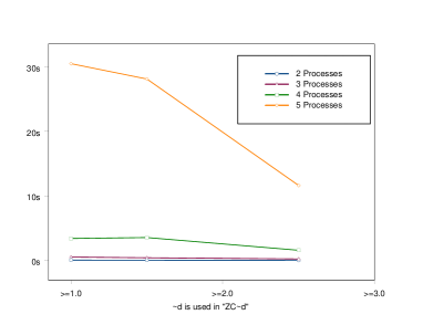
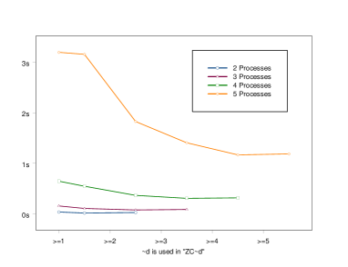
(a) leader-election	(b) PATHOS
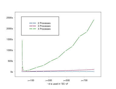
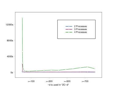
(c) CSMA/CD(A)	(d) CSMA/CD(B)
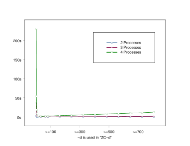
(e) CSMA/CD(C)

The Y-axis is with ”time in sec” while the X-axis is with ”$\sim d$” used in ”$\mbox{\tt ZC}\sim d$.”

Figure 1: Time-complexity charts w.r.t. $d$-values (Data collected with option EDGF)

More charts for the space-complexity can be found in appendix F.

As can be seen from the charts, our algorithms may respond with different complexity curves to various model structures and specifications. For benchmarks leader-election and PATHOS, it seems that the bigger the $d$-value, the better the performance. For the three CSMA/CD benchmarks, it seems that the best performance happens when $d$ is around 80. But one thing common in these charts is that $d=1$ always gives the worst performance.

We have to admit that we do not have a theory to analyze or predict the complexity curves w.r.t. various model structures and specifications. More experiments on more benchmarks may be needed in order to get more understanding of the curves. In general, we feel it can be difficult to analyze such complexity curves. After all, our models of TA are still ”programs” in some sense.

Nevertheless, we have still tried hard to look into the execution of our algorithms for explanation of the complexity cuves. Procedures gfp() and gfp_EDGF() both are constructed with an inner loop (for the least fixpoint evaluation of reachable-bck()) and an outer loop (for the greatest fixpoint evaluation). With bigger $d$-values, it seems that the outer loop converges faster while the inner loop converges slower. That is to say, with bigger $d$-values, we may need less iterations of the outer-loop and, in the same time, more iterations of the inner loop to compute the greatest fixpoints. The complexity patterns in the charts are thus superpositions between the complexities of the outer loop and the inner loop.

We have used the $d$-values with the best performance for the experiments reported in the next few subsections. For benchmarks PATHOS and leader-election, $\sim d$ is set to $>C_{A:\phi}$. ($C_{A:\phi}$ is the biggest timing constant used in model $A$ and TCTL specification $\phi$.) For the three CSMA/CD benchmarks, $\sim d$ is set to $\geq 80$.

9.3 Performance w.r.t. non-Zeno requirement and EDGF

In our first experiment, we observe the performance of our inevitability analysis algorithm w.r.t. the non-Zeno requirement and the EDGF policy. The performance data is in table 1.

		no non-Zeno requirement		non-Zeno requirement
benchmarks	concurrency	EDGF	no EDGF	EDGF	no EDGF
		time/space/answer	time/space/answer	time/space/answer	time/space/answer
pathos	2 proc.s	0.02s/7k/true	0.02s/7k/true	0.03s/7k/true	0.03s/7k/true
	3 proc.s	0.09s/18k/true	0.1s/18k/true	0.08s/17k/true	0.09s/17k/true
	4 proc.s	0.63s/74k/true	0.66s/74k/true	0.31s/42k/true	0.31s/42k/true
	5 proc.s	6.52s/857k/true	6.65s/859k/true	1.17s/114k/true	1.28s/114k/true
	6 proc.s	161s/15087k/true	162s/15090k/true	5.22s/314k/true	5.37s/314k/true
	7 proc.s	O/M	O/M	30.71s/942k/true	31.16s/941k/true
leader	2 proc.s	0.04s/10k/true	0.03s/10k/true	0.04s/16k/true	0.04s/16k/true
election	3 proc.s	0.28s/33k/true	0.28s/33k/true	0.25s/84k/true	0.24s/84k/true
	4 proc.s	1.96s/84k/true	1.98s/84k/true	1.54s/338k/true	1.53s/338k/true
	5 proc.s	10.01s/23/true	10.07s/234k/true	11.23s/1164k/true	11.17s/1164k/true
	6 proc.s	52.63s/635k/true	48.28s/635k/true	110.9s/7992k/true	110.2s/7992k/true
	7 proc.s	206.7s/1693k/true	205.7s/1693k/true	860.5s/42062k/true	859.7s/42062k/true
CSMA/CD	bus+2 senders	0.07s/25k/true	0.15s/25k/true	0.33s/42k/true	9.29s/90k/true
(A)	bus+3 senders	0.24s/49k/true	0.66s/63k/true	3.09s/191k/true	98.33s/191k/true
	bus+4 senders	0.78s/131k/true	2.38s/201k/true	26.23s/936k/true	867.5s/1578k/true
	bus+5 senders	2.39s/378k/true	8.47s/625k/true	195.14s/4501k/true	6021s/7036k
CSMA/CD	bus+2 senders	0.16s/25k/maybe	0.16s/25k/maybe	1.92s/37k/true	2.3s/37k/true
(B)	bus+3 senders	1.52s/62k/maybe	1.52s/62k/maybe	28.67s/151k/true	34.88s/151k/true
	bus+4 senders	10.94s/239k/maybe	11.58s/239k/maybe	235.48s/765k/true	283s/766k/true
CSMA/CD	bus+2 senders	0.05s/25k/true	0.06s/25k/true	0.06s/25k/true	0.72s/36k/true
(C)	bus+3 senders	0.14s/49k/true	0.21s/49k/true	0.29s/79k/true	5.51s/183k/true
	bus+4 senders	0.43s/97k/true	0.67s/97k/true	1.36s/298k/true	30.99s/752k/true
	bus+5 senders	1.32s/286k/true	2.44s/285k/true	6.73s/1045k/true	173.82s/2724k/true
	bus+6 senders	4.57s/833k/true	8.68s/835k/true	33.53s/3436k/true	907.41s/9031k/true
	bus+7 senders	16.32s/2364k/true	32.84s/2367k/true	166.14s/10652k/true	4558s/27993k/true

Table 1: Performance w.r.t. non-Zeno requirements and EDGF techniques

In general, we find that with or without EDGF technique, a non-Zeno requirement does add more complexity to the evaluation of the inevitability properties. Especially for the three specifications of CSMA/CD model, exponential blow-ups have been observed.

For PATHOS benchmark, it is a totally different story. The non-Zeno requirement seems to incur much less complexity than without it. After we have carefully traced the execution of our mode-checker, we found that this benchmark incurs very few iterations of loop (5) in gfp_EDGF() although each iteration can be costly to run. On the other hand, it incurs a significant number of iterations of loop (6) in gfp_Zeno_EDGF() although each iteration is not so costly. The accumulative effect of the loop iterations result in performance that contradicts our expectation. This benchmark shows that the evaluation performance of inevitability properties is very involved and depends on many factors.

Futhermore, benchmark CSMA/CD (B) shows that some inevitability properties can only be verified with non-Zeno computations.

As for the performance of the EDGF technique, we find that when the technique fails, it only incurs a small overhead. When it succeeds, it significantly improves performance two to three-fold.

9.4 Performance w.r.t. abstraction techniques

In table 2, we report the performance data of our red 4.1 with respect to our three abstraction techniques.

benchmarks	concurrency	no abstraction	Game-abs.	Game-discrete-abs.	Game-mag.-abs.
		time/space/answer	time/space/answer	time/space/answer	time/space/answer
pathos	2 procs.s	0.03s/7k/true	0.01s/7k/true	0.03s/7k/true	0.03s/7k/true
	3 procs.s	0.08s/17k/true	0.11s/17k/maybe	0.09s/17k/true	0.1s/22k/true
	4 procs.s	0.31s/42k/true	0.36s/36k/maybe	0.37s/36k/true	0.78s/100k/true
	5 procs.s	1.17s/114k/true	1.16s/71k/maybe	1.2s/71k/true	8.55s/674k/true
	6 procs.s	5.22s/314k/true	2.83s/114k/maybe	3.39s/114k/true	191.1s/6074k/true
	7 procs.s	30.71s/942k/true	6.66s/175k/maybe	8.62s/175k/true	6890s/62321k/true
leader	2 procs.s	0.04s/16k/true	0.03s/16k/true	0.03s/16k/true	0.02s/16k/true
election	3 procs.s	0.25s/84k/true	0.25s/84k/true	0.23s/84k/true	0.25s/84k/true
	4 procs.s	1.54s/338k/true	1.53s/338k/true	1.54s/338k/true	1.52s/338k/true
	5 procs.s	11.23s/1164k/true	11.71s/1164k/true	11.38s/1164k/true	11.39s/1164k/true
	6 procs.s	110.9s/7992k/true	111.2s/7993k/true	110.8s/7993k/true	110.2s/7993k/true
	7 procs.s	860.6s/42062k/true	854.8s/42123k/true	861.5s/42123k/true	867.7s/42123k/true
CSMA/CD	bus+2 senders	0.33s/42k/true	0.33s/42k/true	0.29s/42k/true	0.33s/42k/true
(A)	bus+3 senders	3.09s/191k/true	3.35s/191k/maybe	1.33s/191k/true	3.35s/191k/maybe
	bus+4 senders	26.23s/936k/true	9.57s/731k/maybe	4.79s/731k/true	9.57s/731k/maybe
	bus+5 senders	195.14s/4501k/true	29.89s/2529k/maybe	16.96s/2529k/true	29.8s/2529k/maybe
CSMA/CD	bus+2 senders	1.92s/37k/true	0.58s/25k/true	0.76s/25k/true	0.58s/25k/true
(B)	bus+3 senders	28.67s/151k/true	2.73s/88k/true	3.91s/85k/true	2.73s/88k/true
	bus+4 senders	235.48s/765k/true	9.54s/290k/true	14.72s/281k/true	9.54s/290/true
CSMA/CD	bus+2 senders	0.06s/25k/true	0.06s/25k/true	0.05s/25k/true	0.06s/25k/true
(C)	bus+3 senders	0.29s/79k/true	0.19s/79k/true	0.18s/79k/true	0.19s/79k/true
	bus+4 senders	1.36s/298k/true	0.71s/298k/true	0.73s/298k/true	0.71s/298k/true
	bus+5 senders	6.73s/1045k/true	2.85s/1045k/true	2.90s/1045k/true	2.85s/1045k/true
	bus+6 senders	33.53s/3436k/true	11.84s/3436k/true	11.77s/3436k/true	11.84s/3436k/true
	bus+7 senders	166.14s/10652k/true	47.64s/10652k/true	47.84s/10652k/true	47.64s/10652k/true

All benchmarks run with non-Zeno requirement and EDGF on.

Table 2: Performance w.r.t. abstraction techniques

In general, the abstraction techniques give us much better performance. Notably, game-discrete and game-magnitude abstractions seem to have enough accuracy to discern true properties.

It is somewhat surprising that the game-magnitude abstraction incurs excessive complexity for PATHOS benchmark. After carefully examining the traces generated by red, we found that because non-magnitude constraints were eliminated, some of the inconsistent convex state-spaces in the representation became consistent. These spurious convex state-spaces make many more paths in our CRD and greately burden our greatest fixpoint calculation. For instance, the outer-loop (5) of procedure gfp_EDGF() takes two iterations to reach the fixpoint with the game-magnitude abstraction. It only takes one iteration to do so without the abstraction. In our previous experience, this abstraction has worked efficiently with reachability analysis. It seems that the performance of abstraction techniques for greatest fixpoint evaluation can be subtle.

9.5 Performance w.r.t. Kronos

In table 3, we report the performance of Kronos 5.2 w.r.t. the five benchmarks.

benchmarks	concurrency	no abstraction	extrapolation	inclusion	convex-hull
		time/space/answer	time/space/answer	time/space/answer	time/space/answer
pathos	2 procs	0.0s/true	0.0s/true	0.0s/true	0.0s/true
	3 procs	0.01s/true	0.01s/true	0.02s/true	0.02s/true
	4 procs	Q/N/C	Q/N/C	Q/N/C	Q/N/C
leader	2 procs	0.0s/true	0.0s/true	0.0s/true	0.0s/true
election	3 procs	0.01s/true	0.01s/true	0.01s/true	0.01s/true
	4 procs	0.05s/true	0.06s/true	0.04s/true	0.04s/true
	5 procs	Q/N/C	Q/N/C	Q/N/C	Q/N/C
CSMA/CD	bus+2 senders	0.0s/true	0.01s/true	0.0s/true	0.01s/true
(A)	bus+3 senders	0.01s/true	0.01s/true	0.01s/true	0.01s/true
	bus+4 senders	0.06s/true	0.06s/true	0.06s/true	0.06s/true
	bus+5 senders	0.31s/true	0.31s/true	0.32s/true	0.32s/true
CSMA/CD	bus+2 senders	8.67s/true	8.68s/true	8.65s/true	8.71s/true
(B)	bus+3 senders	O/M	O/M	O/M	O/M
CSMA/CD	bus+2 senders	2.69s/true	2.70s/true	2.72s/true	2.69s/true
(C)	bus+3 senders	O/M	O/M	O/M	O/M

Q/N/C means that Kronos cannot construct the quotient automata.

Table 3: Performance of Kronos in comparison

For PATHOS and leader election, Kronos did not succeed in constructing the quotient automata. But our red seems to have no problem in this regard with its on-the-fly exploration of the state-space. Of course, the lack of high-level data-variables in Kronos’ modeling language may also acerbate the problem.

As for benchmark CSMA/CD (A), Kronos performs very well. We believe this is because this benchmark uses a bounded inevitability specification. Such properties have already been studied in the literature of Kronos[40].

On the other hand, benchmarks CSMA/CD (B) and (C) use unbounded inevitability specifications with modal-subformula nesting depths 1 and 2 respectively. Kronos does not scale up to the complexity of concurrency for these two benchmarks. Our red prevails in these two benchmarks.

10 Conclusion

How to enhance the performance of TCTL model-checking is a research issue to which people have not paid much attention. The reason may be that the reachability analysis problem for TA is already difficult enough and has absorbed much of our energy. Nevertheless, the issue is still important both theoretically and practically. Hopefully, this work can give us some insight to the complexity of the issue and attract more research interest in this regard. Specifically, the charts reported in subsection 9.2 may imply that further research is needed to investigate how to predict good $d$-values in real-world verification tasks. Our implementation shows that the ideas in this paper can be of potential use.

APPENDICES

Appendix A Procedure clock_elimiante()

  $\mbox{\tt clock\_eliminate}(\eta,x)$ {
    for each $x_{1}-x\sim c$ and $x-x_{2}\sim^{\prime}c^{\prime}$, if $\eta\wedge x_{1}-x\sim c\wedge x-x_{2}\sim^{\prime}c^{\prime}$ is not empty, {
       $\eta_{1}:=\eta\wedge x_{1}-x\sim c\wedge x-x_{2}\sim^{\prime}c$;
       $\eta:=\eta\wedge\neg\eta_{1}$; $\eta:=\eta\vee(\eta_{1}\wedge x_{1}-x_{2}\mbox{\tt compose\_upperbound}(\sim,c,\sim^{\prime},c^{\prime}))$;
    }
    return $\eta$;
}
$\mbox{\tt compse\_upperbound}(\sim,c,\sim^{\prime},c^{\prime})$ {
    if $c=\infty\vee c^{\prime}=\infty$, return ”$<\infty$”
    else if $c=-\infty$,
       if $c^{\prime}\leq 0$, return ”$<-\infty$”; else return ”$<-C_{A:\phi}+c^{\prime}$;”
    else if $c^{\prime}=-\infty$,
       if $c\leq 0$, return ”$<-\infty$”; else return ”$<-C_{A:\phi}+c$;”
    $c_{r}:=c+c^{\prime}$;
    if $c_{r}>C_{A:\phi}\vee(\sim_{r}=\mbox{"$<$"}\vee c_{r}=C_{A:\phi})$, return ”$<\infty$;”
    if either $\sim$ or $\sim^{\prime}$ is ”$<$”, $\sim_{r}$ is assigned ”$<$”, else $\sim_{r}$ is assigned ”$\leq$”
    else if $c_{r}<-C_{A:\phi}\vee(\sim_{r}=\mbox{"$<$"}\vee c_{r}=-C_{A:\phi})$, return ”$<-\infty$;”
    else return ”$\sim_{r}c_{r}$”;
}  

Procedure compose_upperbound() computes the new upperbound as the result of adding two, up to the absolute bound of $C_{A:\phi}$. For example, with $C_{A:\phi}=5$, $\mbox{\tt compose\_upperbound}(<,2,\leq,3)=\mbox{"$<\infty$"}$ and $\mbox{\tt compose\_upperbound}(\leq,2,\leq,1)=\mbox{"$\leq 3$"}$.

Appendix B Complete model-checking procedure with non-Zeno requirement

  $\mbox{\tt model-check}(A,\phi)$ {
    if $\mbox{\tt Eval}(A,\emptyset,\neg\phi)$ is false, return true; else return false.
}
$\mbox{\tt Eval}(A,\chi,\bar{\phi})$
/* $\chi$ is the set of clocks declared in the scope of $\bar{\phi}$ */ {
    switch ($\bar{\phi}$) {
    case (false): return false;
    case ($p$): return $p\wedge\bigwedge_{x\in\chi}x\geq 0$;
    case ($x-y\sim c$): return $x-y\sim c\wedge_{x\in\chi}x\geq 0$;
    case ($\phi_{1}\vee\phi_{2}$): return $\mbox{\tt Eval}(A,\chi,\phi_{1})\vee\mbox{\tt Eval}(A,\chi,\phi_{2})$;
    case ($\phi_{1}\wedge\phi_{2}$):
       return $\mbox{\tt Eval}(A,\chi,\phi_{1})\wedge\mbox{\tt Eval}(A,\chi,\phi_{2})$;
    case ($\neg\phi_{1}$): return $\neg\mbox{\tt Eval}(A,\chi,\phi_{1})$;
    case ($x.\phi_{1}$): return $\mbox{\tt clock\_eliminate}(x=0\wedge\mbox{\tt Eval}(A,\chi\cup\{x\},\phi_{1}\wedge x\geq 0),x)$;
    case ($\exists\phi_{1}\mbox{$\cal U$}\phi_{2}$):
       $\eta_{1}:=\mbox{\tt Eval}(A,\chi,\phi_{1})$; $\eta_{2}:=\mbox{\tt Eval}(A,\chi,\phi_{2})$;
       return $\mbox{\tt reachable-bck}(\eta_{1},\eta_{2})$;
    case ($\exists\Box\phi_{1}$): return $\mbox{\tt gfp}(\mbox{\tt Eval}(A,\phi_{1}))$;
    }
}  

Appendix C Abstract model-checking with TCTL^∀

In the application of abstraction techniques, it is important to make them safe[39]. That is to say, when the safe abstraction analyzer says a property is true, the property is indeed true. (But when it says false, we do not know whether the property is true.) There are two types of abstractions: over-approximation and under-approximation. The former means that the abstract state-space is a superset of the concrete state-space, while the latter means that the abstract state-space is a subset of the concrete state-space. To make an abstraction safe means that we should stick to over-approximation while evaluating $\exists\Box\neg\phi$ (the negation of the inevitability). But this can be difficult to enforce in general since negations deeply nested in formulas can turn over-approximation into under-approximation and thus make abstractions unsafe.

Usually inevitability properties do not occur on their own either. Instead, they are usually nested in other modal-formulas. For example, normally we may specify that

When there is a request, then eventually there is a service.

In TCTL, this can be written as

$\forall\Box\left(\mbox{\tt request}\rightarrow\forall\Diamond\mbox{\tt service}\right)$ $(f1)$

In general, it can be difficult to restrict the negation of over-approximation from happening. But fortunately, formula $(f1)$ does not have such a problem. Consider the negation of formula $(f1)$, which is the following.

$\exists\Diamond\left(\mbox{\tt request}\wedge\exists\Box\neg\mbox{\tt service}\right)$ $(f2)$

Since there is no negation sign before any modal-formula, there is no problem with negation of over-approximation. Thus over-approximation can be applied here by doing over-approximations of the state sets thus satisfying the following subformulas in sequence (from left to right).

$\neg\mbox{\tt service},\;\exists\Box\neg\mbox{\tt service},\;\mbox{\tt request},\;\mbox{\tt request}\wedge\exists\Box\neg\mbox{\tt service},\;(f2),\;I\wedge(f2)$

If the state-set for $I\wedge(f2)$ is empty, then formula $(f1)$ is satisfied; else we do not have a conclusion. Note that the evaluation of state sets for $\neg\mbox{\tt service}$ and request respectively does not need any abstraction.

The reasoning in the last paragraph can be extended to a general subclass of TCTL, TCTL^∀. A formula is in TCTL^∀iff the negation signs only appear before its atoms, and only universal path quantifications are used. For example, we may want to verify the following specification:

$\forall\Box\left(\mbox{\tt request}\rightarrow\forall\Box\left(\mbox{\tt service}\rightarrow\forall\Diamond\mbox{\tt request}\right)\right)$

The formula says that if there is a request followed by a service, then from that service on, there will be a request. The negation of the specification is $\exists\Diamond\left(\mbox{\tt request}\wedge\exists\Diamond\left(\mbox{\tt service}\wedge\exists\Box\neg\mbox{\tt request}\right)\right)$, which is in the subclass of TCTL^∃, the subclass of TCTL with negations right before atoms and with only existential path quantifications. Note that the negations of formulas in TCTL^∀ fall correctly in TCTL^∃. The following lemma shows that over-approximation techniques with TCTL^∃formulas always yield over-approximation.

Lemma 7

: Given a TCTL^∃formula $\phi$, if we evaluate each modal-subformula in $\phi$ with over-approximation, then we still get an over-approximation of the state set satisfying $\phi$.

Proof : This can be done by an inductive analysis on the structure of $\phi$. If $\phi$ is a literal expression of the forms $p$ or $\neg p$, then the evaluation does not involve any approximation. If $\phi$ is like $\phi_{1}\vee\phi_{2}$ or $\phi_{1}\wedge\phi_{2}$, then the evaluation of $\phi$ still yields over-approximation with the inductive hypothesis that the evaluations of $\phi_{1}$ and $\phi_{2}$ are both over-approximations. If $\phi$ is like $\exists\phi_{1}\mbox{$\cal U$}\phi_{2}$, then since the modal-formula is to be evaluated with over-approximation, with the inductive hypothesis, we know that $\phi$ is evaluated with over-approximation. The case for $\exists\Box\phi_{1}$ is similar. Thus the lemma is proven.     $\blacksquare$

Our over-approximation technique is directly applied in procedure $\mbox{\tt reachable-bck}()$. In other words, we can extend $\mbox{\tt reachable-bck}()$ with over-approximation techniques as following.

$\mbox{\tt reachable-bck}^{O}(\eta_{1},\eta_{2})\equiv\mbox{\tt lfp}Y.\mbox{\tt abs}\left(\eta_{2}\vee\left(\eta_{1}\wedge\mbox{\tt time\_bck}(\eta_{1}\wedge\bigvee_{e\in T}\mbox{\tt xtion\_bck}(Y,e))\right)\right)$.

Here $\mbox{\tt abs}()$ means a generic over-approximation procedure. Thus procedure $\mbox{\tt reachable-bck}^{O}()$ can be used in place of $\mbox{\tt reachable-bck}()$ in procedures gfp(), Eval-EDGF(), and gfp_EDGF().

In our tool red 4.1, we have implemented a series of game-based abstraction procedures suitable for BDD-like data-structures and concurrent systems[38]. We use the term ”game” here because we envision the concurrent system operation as a game. Those processes, which we want to verify, are treated as players while the other processes are treated as opponents. In the game, the players try to win (maintain the specification property) under the worst (i.e., minimal) assumption on their opponents. A process is a player iff its local variables appear in the inevitability properties. The other processes are called opponents. According to the well-observed discipline of modular programming[30], the behavioral correctness of a functional module should be based on minimal assumption on the environment. These game-based abstraction procedures omit opponents’ state-information to make abstractions.

• Game-abstraction: The game abstraction procedure will eliminate the state information of the opponents from its argument state-predicate.

• Game-discrete-abstraction: This abstraction procedure will eliminate all clock constraints for the opponents in the argument state-predicate.

• Game-magnitude-abstraction: A clock constraint like $x-x^{\prime}\sim c$ is called a magnitude constraint iff either $x$ or $x^{\prime}$ is zero itself (i.e. the constraint is either $x\sim c$ or $-x^{\prime}\sim c$). This abstraction procedure will erase all non-magnitude constraints of the opponents in the argument state-predicate.

Details can be found in [38].

Appendix D Benchmarks

We use the following benchmarks to test our ideas and implementations. The specifications for the benchmarks fall in TCTL^∀. Thus we can also carry out experiments with our abstraction techniques.

• PATHOS real-time operating system scheduling specification[4]:
  In the system, each process runs with a distinct priority in a period equal to the number of processes. The biggest timing constant used is equal to the number of processes. The unbounded inevitability property we want to evaluate is that ”if the process with lowest priority is in the pending state, then inevitably it will enter the running state thereafter.” For a system with three processes, this property is as follows.

  $\forall\Box\left(\mbox{\tt pending}_{3}\rightarrow\forall\Diamond\mbox{\tt running}_{3}\right)$

  The nesting depth of the modal-operators is one.

• Leader election specification[35]:
  Each process has a local pointer parent and a local clock. All processes initially come with its parent = NULL. Then a process with its parent = NULL may broadcast its request to be adopted by a parent. Another process with its parent = NULL may respond. The process with the smaller identifier will become the parent of the other process in the requester-responder pair. The biggest timing constant used is $2$. The unbounded inevitability we want to verify is that eventually, the algorithm will finish with a unique leader elected. That is

  $\forall\Diamond\left(\mbox{\tt parent}_{1}=\mbox{\tt NULL}\wedge\forall i:i\neq 1,\left(\mbox{\tt parent}_{i}\neq\mbox{\tt NULL}\wedge\mbox{\tt parent}_{i}<i\right)\right)$

  There is no nested modal-operators. To guarantee the inevitability, we assume that a process with parent = NULL will finish an iteration of the algorithm in 2 time units.

• CSMA/CD protocol [33, 34, 40]:
  Basically, this is the ethernet bus arbitration protocol with the idea of collision-and-retry. The timing constants used are 26, 52, and 808. We have used three TCTL specifications for these benchmarks.

  • The first one requires that, when two processes are simultaneously in the transmission mode, then in 26 time units, the bus will inevitably go back to the idle state. The property is a bounded inevitability and can be written as follows:

    $\forall\Box\left(\left(\mbox{\tt transm}_{1}\wedge\mbox{\tt transm}_{2}\right)\rightarrow x.\forall\Diamond\left(x<26\wedge\mbox{\tt bus\_idle}\right)\right)$ (A)

    Note that the inevitability is timed to happen in 26 time units. This experiment allows us to observe how our techniques perform with bounded inevitability.

  • The second specification requires that if sender 1 is in its transmission mode for no less than 52 time units, then it will inevitably enter the wait mode.

    $\forall\Box((\mbox{\tt transm}_{1}\wedge x_{1}\geq 52)\rightarrow\forall\Diamond\mbox{\tt wait}_{1})$ (B)

    Specially, this specification can only be verified by quantifying only on non-Zeno computations.

  • The third specification requires that if the bus is in the idle mode and later enters the collision mode, then it will inevitably go back to the idle mode. This unbounded inevitability property is as follows.

    $\forall\Box\left(\mbox{\tt bus\_idle}\rightarrow\forall\Box\left(\mbox{\tt bus\_collision}\rightarrow\forall\Diamond\mbox{\tt bus\_idle}\right)\right)$ (C)

    This property is special in that the nesting depth of modal-operator is two and can give us some insight on how our abstraction techniques scale to the inductive structure of specifications.

Appendix E Performance data w.r.t. $d$-values

The performance data with various $d$-value setting in the evaluation of greatest fixpoint with non-Zeno computation requirement is in table 4.

benchmarks	$d$-values	2 procs	3 procs	4 procs	5 procs
		time/space	time/space	time/space	time/space
leader	$>$2	0.03s/16k	0.24s/84k	1.58s/338k	11.625s/1164k
	$>$1	0.04s/16k	0.42s/89k	3.55s/482k	28.15s/1612k
	$>=$1	0.05s/16k	0.53s/88k	3.41s/451k	30.52s/1554k
patho	$>$5	not available			1.19s/114k
	$>$4			0.32s/42k	1.17s/109k
	$>$3		0.09s/17k	0.31s/41k	1.41s/119k
	$>$2	0.03s/7k	0.08s/17k	0.37s/51k	1.83s/221k
	$>$1	0.02s/7k	0.11s/21k	0.55s/76k	3.16s/244k
	$>=$1	0.04s/7k	0.16s/26k	0.65s/76k	3.2s/245k
CSMA/CD	$>$808	1.14s/45k	93s/1418k	2394.12s/10936k
(A)	$>$646	0.94s/44k	65.63s/1232k	1616.22s/8581k
	$>$404	0.72s/43k	34.36s/877k	636.53s/5336k
	$>$161	0.54s/42k	13.24s/501k	185.17s/2539k
	$>$80	0.45s/42k	6.63s/308k	65.41s/1483k
	$>=$64	0.46s/42k	5.3s/259k	51.77s/1230k
	$>=$32	0.34s/42k	3.22s/191k	27.16s/936k
	$>=$16	0.70s/82k	6.58s/426k	55.5s/1640k
	$>=$8	1.43s/96k	14.5s/510k	123.68s/1958k
	$>=$4	2.66s/118k	28.37s/639k	255.59s/2446k
	$>=$2	5.54s/165k	62s/900k	516.76s/3430k
	$>=$1	15.64s/270k	186.86s/1480k	1443.97s/5587k
CSMA/CD	$>$808	0.66s/35k	34s/719k	863.29s/5198k
(B)	$>$646	1.38s/62k	48.45s/658k	1095.99s/4187k
	$>$323	1.15s/40k	31.14s/421k	507.73s/2178k
	$>$161	1.27s/37k	26.61s/265k	320.67s/1199k
	$>$80	1.91s/37k	29.08s/151k	240.77s/765k
	$>=$64	2.22s/37k	28.01s/130k	240.44s/631k
	$>=$32	3.51s/56k	36.31s/228k	272.32s/801k
	$>=$16	6.45s/59k	69.62s/251k	521.32s/875k
	$>=$8	13.88s/67k	143.44s/280k	1068s/958k
	$>=$4	30.22s/80k	309.2s/326k	2257s/1087k
	$>=$2	73.32s/113k	717.8s/423k	5165s/1349k
	$>=$1	230s/214k	2119s/667k	13630s/1951k
CSMA/CD	$>$808	0.19s/25k	1.75s/80k	12.7s/300k
(C)	$>$646	0.17s/25k	1.48s/80k	10.09s/299k
	$>$404	0.13s/25k	1s/80k	6.52s/299k
	$>$161	0.08s/25k	0.6s/80k	3.68s/299k
	$>$80	0.07s/25k	0.4s/80k	2.12s/299k
	$>=$64	0.08s/25k	0.42s/80k	2.27s/299k
	$>=$32	0.07s/25k	0.32s/79k	1.55s/298k
	$>=$16	0.11s/36k	0.66s/192k	3.12s/863k
	$>=$8	0.22s/47k	1.51s/256k	7.96s/1056k
	$>=$4	0.44s/64k	3.16s/355k	18.61s/1438k
	$>=$2	1.03s/98k	9.07s/556k	53.9s/2208k
	$>=$1	3.3s/178k	37.11s/1001k	230.32s/3892k

Table 4: Performance w.r.t. $d$-values

Appendix F Space complexity charts w.r.t. $d$-values

The charts for memory complexity with various $d$-parameter values is in figure 2.

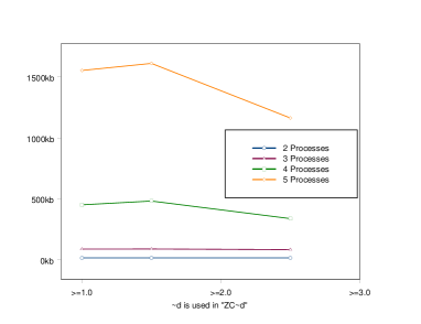
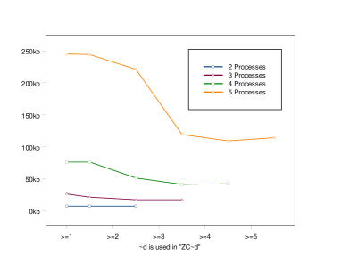
(a) leader-election	(b) PATHOS
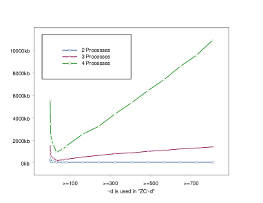
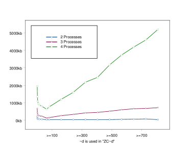
(c) CSMA/CD(A)	(d) CSMA/CD(B)
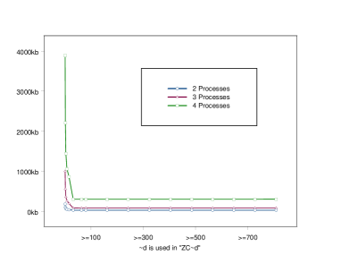
(e) CSMA/CD(C)

The Y-axis is with ”memory space in kb” while the X-axis is with ”$\sim d$” used in ”$\mbox{\tt ZC}\sim d$.”

Figure 2: Memory-complexity charts w.r.t. $d$-values (Data collected with option EDGF)

References

- [1] R. Alur, C. Courcoubetis, D.L. Dill. Model Checking for Real-Time Systems, IEEE LICS, 1990.
- [2] R. Alur, D.L. Dill. Automata for modelling real-time systems. ICALP’ 1990, LNCS 443, Springer-Verlag, pp.322-335.
- [3] B. Alpern, F.B. Schneider. Defining Liveness. Information Processing Letters 21, 4 (October 1985), 181-185.
- [4] F. Balarin. Approximate Reachability Analysis of Timed Automata. IEEE RTSS, 1996.
- [5] J.R. Burch, E.M. Clarke, K.L. McMillan, D.L.Dill, L.J. Hwang. Symbolic Model Checking: States and Beyond, IEEE LICS, 1990.
- [6] J. Bengtsson, K. Larsen, F. Larsson, P. Pettersson, Wang Yi. UPPAAL - a Tool Suite for Automatic Verification of Real-Time Systems. Hybrid Control System Symposium, 1996, LNCS, Springer-Verlag.
- [7] G. Behrmann, K.G. Larsen, J. Pearson, C. Weise, Wang Yi. Efficient Timed Reachability Analysis Using Clock Difference Diagrams. CAV’99, July, Trento, Italy, LNCS 1633, Springer-Verlag.
- [8] R.E. Bryant. Graph-based Algorithms for Boolean Function Manipulation, IEEE Trans. Comput., C-35(8), 1986.
- [9] P. Cousot, R. Cousot. Abstract Interpretation: a Unified Lattice Model for Static Analysis of Programs of by Construction or Approximation of Fixpoints. 4th ACM POPL, January 1977.
- [10] P. Cousot, R. Cousot. Abstract Interpretation and application to logic programs. Journal of Logic Programming, 13(2-3):103-179, 1992.
- [11] E. Clarke, E.A. Emerson, Design and Synthesis of Synchronization Skeletons using Branching-Time Temporal Logic, in ”Proceedings, Workshop on Logic of Programs,” LNCS 131, Springer-Verlag.
- [12] E. Clarke, E.A. Emerson, A.P. Sistla. Automatic Verification of Finite-State Concurrent Systems using Temporal-Logic Specifications, ACM Trans. Programming, Languages, and Systems, 8, Nr. 2, pp. 244–263.
- [13] E. Clarke, O. Grumberg, S. Jha, Y. Lu, H. Veith. Counterexample-guided Abstraction Refinement. CAV’2000.
- [14] D.L. Dill. Timing Assumptions and Verification of Finite-state Concurrent Systems. CAV’89, LNCS 407, Springer-Verlag.
- [15] C. Daws, A. Olivero, S. Tripakis, S. Yovine. The tool KRONOS. The 3rd Hybrid Systems, 1996, LNCS 1066, Springer-Verlag.
- [16] E.A. Emerson. Uniform Inevitability is tree automataon ineffable. Information Processing Letters 24(2), Jan 1987, pp.77-79.
- [17] T.A. Henzinger, X. Nicollin, J. Sifakis, S. Yovine. Symbolic Model Checking for Real-Time Systems, IEEE LICS 1992.
- [18] C.A.R. Hoare. Communicating Sequential Processes, Prentice Hall, 1985.
- [19] P.-A. Hsiung, F. Wang. User-Friendly Verification. Proceedings of 1999 FORTE/PSTV, October, 1999, Beijing. Formal Methods for Protocol Engineering and Distributed Systems, editors: J. Wu, S.T. Chanson, Q. Gao; Kluwer Academic Publishers.
- [20] F. Laroussinie, K.G. Larsen. CMC: A Tool for Compositional Model-Checking of Real-Time Systems. FORTE/PSTV’98, Kluwer.
- [21] K.G. Larsen, F. Larsson, P. Pettersson, Y. Wang. Efficient Verification of Real-Time Systems: Compact Data-Structure and State-Space Reduction. IEEE RTSS, 1998.
- [22] W. Lee, A. Pardo, J.-Y. Jang, G. Hachtel, F. Somenzi. Tearing Based Automatic Abstraction for CTL Model Checking. ICCAD’96.
- [23] J. Moller, J. Lichtenberg, H.R. Andersen, H. Hulgaard. Difference Decision Diagrams, in proceedings of Annual Conference of the European Association for Computer Science Logic (CSL), Sept. 1999, Madreid, Spain.
- [24] J. Moller, J. Lichtenberg, H.R. Andersen, H. Hulgaard. Fully Symbolic Model-Checking of Timed Systems using Difference Decision Diagrams, in proceedings of Workshop on Symbolic Model-Checking (SMC), July 1999, Trento, Italy.
- [25] Z. Manna, A. Pnueli. Temporal Verification of Reactive Systems: Safety. Springer-Verlag, 1995.
- [26] M.O. Moller. Parking Can Get You There Faster - Model Augmentation to Speed up Real-Time Model Checking. Electronic Notes in Theoretical Computer Science 65(6), 2002.
- [27] A.W. Mazurkiewicz, E. Ochmanski, W. Penczek. Concurrent Systems and Inevitability. TCS 64(3): 281-304, 1989.
- [28] P. Pettersson, K.G. Larsen, UPPAAL2k. in Bulletin of the European Association for Theoretical Computer Science, volume 70, pages 40-44, 2000.
- [29] A. Pnueli, The Temporal Logic of Programs, 18th annual IEEE-CS Symp. on Foundations of Computer Science, pp. 45-57, 1977.
- [30] R.S. Pressman. Software Engineering, A Practitioner’s Approach. McGraw-Hill, 1982.
- [31] F. Wang. Efficient Data-Structure for Fully Symbolic Verification of Real-Time Software Systems. TACAS’2000, March, Berlin, Germany. in LNCS 1785, Springer-Verlag.
- [32] F. Wang. Region Encoding Diagram for Fully Symbolic Verification of Real-Time Systems. the 24th COMPSAC, Oct. 2000, Taipei, Taiwan, ROC, IEEE press.
- [33] F. Wang. RED: Model-checker for Timed Automata with Clock-Restriction Diagram. Workshop on Real-Time Tools, Aug. 2001, Technical Report 2001-014, ISSN 1404-3203, Dept. of Information Technology, Uppsala University.
- [34] F. Wang. Symbolic Verification of Complex Real-Time Systems with Clock-Restriction Diagram, to appear in Proceedings of FORTE, August 2001, Cheju Island, Korea.
- [35] F. Wang. Efficient Verification of Timed Automata with BDD-like Data-Structures. proceedings of VMCAI’2003, LNCS 2575, Springer-Verlag.
- [36] F. Wang, P.-A. Hsiung. Automatic Verification on the Large. Proceedings of the 3rd IEEE HASE, November 1998.
- [37] F. Wang, P.-A. Hsiung. Efficient and User-Friendly Verification. IEEE Transactions on Computers, Jan. 2002.
- [38] F. Wang, G.-D. Hwang, F. Yu. Symbolic Simulation of Real-Time Concurrent Systems. to appear in proceedings of RTCSA’2003, Feb. 2003, Tainan, Taiwan, ROC.
- [39] H. Wong-Toi. Symbolic Approximations for Verifying Real-Time Systems. Ph.D. thesis, Stanford University, 1995.
- [40] S. Yovine. Kronos: A Verification Tool for Real-Time Systems. International Journal of Software Tools for Technology Transfer, Vol. 1, Nr. 1/2, October 1997.