Recent Results on
No-Free-Lunch Theorems for Optimization

Abstract

The sharpened No-Free-Lunch-theorem (NFL-theorem) states that the performance of all optimization algorithms averaged over any finite set $F$ of functions is equal if and only if $F$ is closed under permutation (c.u.p.) and each target function in $F$ is equally likely. In this paper, we first summarize some consequences of this theorem, which have been proven recently: The average number of evaluations needed to find a desirable (e.g., optimal) solution can be calculated; the number of subsets c.u.p. can be neglected compared to the overall number of possible subsets; and problem classes relevant in practice are not likely to be c.u.p. Second, as the main result, the NFL-theorem is extended. Necessary and sufficient conditions for NFL-results to hold are given for arbitrary, non-uniform distributions of target functions. This yields the most general NFL-theorem for optimization presented so far.

1 Introduction

Search heuristics such as evolutionary algorithms, grid search, simulated annealing, and tabu search are general in the sense that they can be applied to any target function $f:\mathcal{X}\to\mathcal{Y}$, where $\mathcal{X}$ denotes a finite search space and $\mathcal{Y}$ is a finite set of totally ordered cost-values. Much research is spent on developing search heuristics that are superior to others when the target functions belong to a certain class of problems. But under which conditions can one search method be better than another? The No-Free-Lunch-theorem for optimization (NFL-theorem) roughly speaking states that all non-repeating search algorithms have the same mean performance when averaged uniformly over all possible objective functions $f:\mathcal{X}\to\mathcal{Y}$ [10, 7, 11, 6, 1]. Of course, in practice an algorithm need not perform well on all possible functions, but only on a subset that arises from the real-world problems at hand, e.g., optimization of neural networks. Recently, a sharpened version of the NFL-theorem has been proven that states that NFL-results hold (i.e., the mean performance of all search algorithms is equal) for any subset $F$ of the set of all possible functions if and only if $F$ is closed under permutation (c.u.p.) and each target function in $F$ is equally likely [8].

In this paper, we address the following basic questions: When all algorithms have the same mean performance—how long does it take on average to find a desirable solution? How likely is it that a randomly chosen subset of functions is c.u.p., i.e., fulfills the prerequisites of the sharpened NFL-theorem? Do constraints relevant in practice lead to classes of target functions that are c.u.p.? And finally: How can the NFL-theorem be extended to non-uniform distributions of target functions? Answers to all these questions are given in the sections 3 to 5. First, the scenario considered in NFL-theorems is described formally.

2 Preliminaries

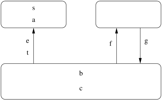
Figure 1: Schema of the optimization scenario considered in NFL-theorems. A non-repeating black-box search algorithm $a$ chooses a new exploration point in the search space depending on the sequence $T_{m}$ of the already visited points with their corresponding cost-values. The target function $f$ returns the cost-value of a candidate solution as the only information. The performance of $a$ is determined using the performance measure $c$, which is a function of the sequence $Y(f,m,a)$ containing the cost-values.

A finite search space $\mathcal{X}$ and a finite set of cost-values $\mathcal{Y}$ are presumed. Let $\mathcal{F}$ be the set of all objective functions $f:\mathcal{X}\to\mathcal{Y}$ to be optimized (also called target, fitness, energy, or cost functions). NFL-theorems are concerned with non-repeating black-box search algorithms (referred to as algorithms) that choose a new exploration point in the search space depending on the history of prior explorations: The sequence $T_{m}=\left<(x_{1},f(x_{1})),(x_{2},f(x_{2})),\dots,(x_{m},f(x_{m}))\right>$ represents $m$ pairs of different search points $x_{i}\in\mathcal{X}$, $\forall{i,j}:\,x_{i}\not=x_{j}$ and their cost-values $f(x_{i})\in\mathcal{Y}$. An algorithm $a$ appends a pair $(x_{m+1},f(x_{m+1}))$ to this sequence by mapping $T_{m}$ to a new point $x_{m+1}$, $\forall{i}:\,x_{m+1}\not=x_{i}$. In many search heuristics, such as evolutionary algorithms or simulated annealing in their canonical form, it is not ensured that a point in the search space is evaluated only once. However, these algorithms can become non-repeating when they are coupled with a search-point database, see [3] for an example in the field of structure optimization of neural networks.

The performance of an algorithm $a$ after $m$ iterations with respect to a function $f$ depends only on the sequence $Y(f,m,a)=\left<f(x_{1}),f(x_{2}),\dots,f(x_{m})\right>$ of cost-values, the algorithm has produced. Let the function $c$ denote a performance measure mapping sequences of cost-values to the real numbers. For example, in the case of function minimization a performance measure that returns the minimum cost-value in the sequence could be a reasonable choice. See Fig. 1 for a schema of the scenario assumed in NFL-theorems.

Using these definitions, the original NFL-theorem for optimization reads:

Theorem 2.1 (NFL-theorem [11])

For any two algorithms $a$ and $b$, any $k\in\mathbbm{R}$, any $m\in\{1,\dots,|\mathcal{X}|\}$, and any performance measure $c$

$$\sum_{f\in\mathcal{F}}\delta(k,c(Y(f,m,a)))=\sum_{f\in\mathcal{F}}\delta(k,c(Y(f,m,b)))\enspace.$$ (1)

Herein, $\delta$ denotes the Kronecker function ($\delta(i,j)=1$ if $i=j$, $\delta(i,j)=0$ otherwise). Proofs can be found in [10, 11, 6]. This theorem implies that for any two (deterministic or stochastic, cf. [1]) algorithms $a$ and $b$ and any function $f_{a}\in\mathcal{F}$, there is a function $f_{b}\in F$ on which $b$ has the same performance as $a$ on $f_{a}$. Hence, statements like “Averaged over all functions, my search algorithm is the best” are misconceptions. Note that the summation in (1) corresponds to uniformly averaging over all functions in $\mathcal{F}$, i.e., each function has the same probability to be the target function.

Recently, theorem 2.1 has been extended to subsets of functions that are closed under permutation (c.u.p.). Let $\pi:\mathcal{X}\rightarrow\mathcal{X}$ be a permutation of $\mathcal{X}$. The set of all permutations of $\mathcal{X}$ is denoted by $\Pi(\mathcal{X})$. A set $F\subseteq\mathcal{F}$ is said to be c.u.p. if for any $\pi\in\Pi(\mathcal{X})$ and any function $f\in F$ the function $f\circ\pi$ is also in $F$.

Example 1

Consider the mappings $\{0,1\}^{2}\to\{0,1\}$, denoted by $f_{0},f_{1},\dots,f_{15}$ as shown in table 1. Then the set $\{f_{1},f_{2},f_{4},f_{8}\}$ is c.u.p., also $\{f_{0},f_{1},f_{2},f_{4},f_{8}\}$. The set $\{f_{1},f_{2},f_{3},f_{4},f_{8}\}$ is not c.u.p., because some functions are “missing”, e.g., $f_{5}$, which results from $f_{3}$ by switching the elements $(0,1)^{T}$ and $(1,0)^{T}$.

Table 1: Functions $\{0,1\}^{2}\to\{0,1\}$.

$(x_{1},x_{2})^{T}$	$f_{0\phantom{0}}$	$f_{1\phantom{0}}$	$f_{2\phantom{0}}$	$f_{3\phantom{0}}$	$f_{4\phantom{0}}$	$f_{5\phantom{0}}$	$f_{6\phantom{0}}$	$f_{7\phantom{0}}$	$f_{8\phantom{0}}$	$f_{9\phantom{0}}$	$f_{10}$	$f_{11}$	$f_{12}$	$f_{13}$	$f_{14}$	$f_{15}$
$(0,0)^{T}$	0	1	0	1	0	1	0	1	0	1	0	1	0	1	0	1
$(0,1)^{T}$	0	0	1	1	0	0	1	1	0	0	1	1	0	0	1	1
$(1,0)^{T}$	0	0	0	0	1	1	1	1	0	0	0	0	1	1	1	1
$(1,1)^{T}$	0	0	0	0	0	0	0	0	1	1	1	1	1	1	1	1

In [8] it is proven:

Theorem 2.2 (sharpened NFL-theorem [8])

For any two algorithms $a$ and $b$, any $k\in\mathbbm{R}$, any $m\in\{1,\dots,|\mathcal{X}|\}$, and any performance measure $c$

$$\sum_{f\in F}\delta(k,c(Y(f,m,a)))=\sum_{f\in F}\delta(k,c(Y(f,m,b)))$$ (2)

iff $F$ is c.u.p.

This is an important extension of theorem 2.1, because it gives necessary and sufficient conditions for NFL-results for subsets of functions. But still theorem 2.2 can only be applied if all elements in $\mathcal{F}$ have the same probability to be the target function, because the summations average uniformly over $F$.

In the following, the concept of $\mathcal{Y}$-histograms is useful. A $\mathcal{Y}$-histogram (histogram for short) is a mapping $h:\,\mathcal{Y}\to{\mathbbm{N}}_{0}$ such that $\sum_{y\in\mathcal{Y}}h(y)=|\mathcal{X}|$. The set of all histograms is denoted $\mathcal{H}$. Any function $f:\,\mathcal{X}\to\mathcal{Y}$ implies the histogram $h_{f}(y)=|f^{-1}(y)|$ that counts the number of elements in $\mathcal{X}$ that are mapped to the same value $y\in\mathcal{Y}$ by $f$. Herein, $f^{-1}(y),y\in\mathcal{Y}$ returns the preimage $\{x|f(x)=y\}$ of $y$ under $f$. Further, two functions $f,g$ are called $h$-equivalent iff they have the same histogram. The corresponding $h$-equivalence class $B_{h}\subseteq\mathcal{F}$ containing all functions with histogram $h$ is termed a basis class.

Example 2

Consider the functions in table 1. The $\mathcal{Y}$-histogram of $f_{1}$ contains the value zero three times and the value one one time, i.e., we have $h_{f_{1}}(0)=3$ and $h_{f_{1}}(1)=1$. The mappings $f_{1}$, $f_{2}$, $f_{4}$, $f_{8}$ have the same $\mathcal{Y}$-histogram and are therefore in the same basis class $B_{h_{f_{1}}}=\{f_{1},f_{2},f_{4},f_{8}\}$. The set $\{f_{1},f_{2},f_{4},f_{8},f_{15}\}$ is c.u.p. and corresponds to $B_{h_{f_{1}}}\cup B_{h_{f_{15}}}$.

It holds:

Lemma 1 ([5])

1. Any subset $F\subseteq\mathcal{F}$ that is c.u.p. is uniquely defined by a union of pairwise disjoint basis classes.

2. $B_{h}$ is equal to the permutation orbit of any function $f$ with histogram $h$, i.e.,

   $$B_{h}=\bigcup_{\pi\in\Pi(\mathcal{X})}\{f\circ\pi\}\enspace.$$ (3)

A proof is given in [5].

3 Time to Find a Desirable Solution

Theorem 2.2 tells us that on average all algorithms need the same time to find a desirable, say optimal, solution—but how long does it take? The average number of evaluations, i.e., the mean first hitting time $\text{E}\{{\mathcal{T}}\}$, needed to find an optimum depends on the cardinality of the search space $|\mathcal{X}|$ and the number ${n}$ of search points that are mapped to a desirable solution.

Let $F_{{n}}\subset\mathcal{F}$ be the set of all functions where ${n}$ elements in $\mathcal{X}$ are mapped to optimal solutions. For non-repeating black-box search algorithms it holds:

Theorem 3.1 ([4])

Given a search space of cardinality $|\mathcal{X}|$ the expected number of evaluations $\text{E}\{{\mathcal{T}}_{|\mathcal{X}|,{n}}\}$ averaged over $F_{{n}}\subseteq\mathcal{F}$ is given by

$$\text{E}\{{\mathcal{T}}_{|\mathcal{X}|,{n}}\}=\frac{|\mathcal{X}|+1}{{n}+1}\enspace.$$ (4)

A proof can be found in [4], where this result is used to study the influence of neutrality (i.e., of non-injective genotype-phenotype mappings) on the time to find a desirable solution.

4 Fraction of Subsets Closed under Permutation

The NFL-theorems can be regarded as the basic skeleton of combinatorial optimization and are important for deriving theoretical results as the one presented in the previous section. However, are the preconditions of the NFL-theorems ever fulfilled in practice? How likely is it that a randomly chosen subset is c.u.p.?

There exist $2^{\left(|\mathcal{Y}|^{|\mathcal{X}|}\right)}-1$ non-empty subsets of $\mathcal{F}$ and it holds:

Theorem 4.1 ([5])

The number of non-empty subsets of $\mathcal{Y}^{\mathcal{X}}$ that are c.u.p. is given by

$$2^{\binom{|\mathcal{X}|+|\mathcal{Y}|-1}{|\mathcal{X}|}}-1$$ (5)

and therefore the fraction of non-empty subsets c.u.p. is given by

$$\left({2^{\binom{|\mathcal{X}|+|\mathcal{Y}|-1}{|\mathcal{X}|}}-1}\right)\Big{/}\left({2^{\left(|\mathcal{Y}|^{|\mathcal{X}|}\right)}-1}\right)\enspace.$$ (6)

The proof is given in [5].

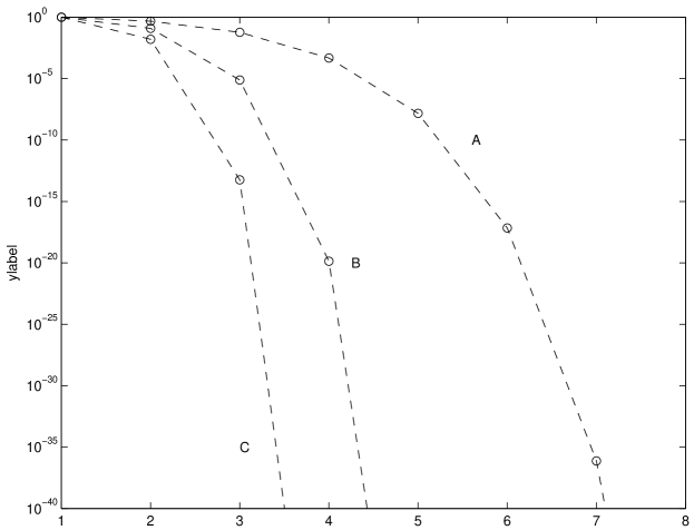
Figure 2: The ordinate gives the fraction of subsets closed under permutation on logarithmic scale given the cardinality of the search space $\mathcal{X}$. The different curves correspond to different cardinalities of the codomain $\mathcal{Y}$.

Figure 2 shows a plot of the fraction of non-empty subsets c.u.p. versus the cardinality of $\mathcal{X}$ for different values of $|\mathcal{Y}|$. The fraction decreases for increasing $|\mathcal{X}|$ as well as for increasing $|\mathcal{Y}|$. More precisely, for $|\mathcal{Y}|>e|\mathcal{X}|/(|\mathcal{X}|-e)$ it converges to zero double exponentially fast with increasing $|\mathcal{X}|$. Already for small $|\mathcal{X}|$ and $|\mathcal{Y}|$ the fraction almost vanishes.

Thus, the statement “I’m only interested in a subset $F$ of all possible functions, so the precondition of the sharpened NFL-theorems is not fulfilled” is true with a probability close to one (if $F$ is chosen uniformly and $\mathcal{Y}$ and $\mathcal{X}$ have reasonable cardinalities). The fact that the precondition of the NFL-theorem is violated does not lead to “Free Lunch”, but nevertheless ensures the possibility of a “Free Appetizer”.

5 Search Spaces with Neighborhood Relations

Although the fraction of subsets c.u.p. is close to zero already for small search and cost-value spaces, the absolute number of subsets c.u.p. grows rapidly with increasing $|\mathcal{X}|$ and $|\mathcal{Y}|$. What if these classes of functions are the relevant ones, i.e., those we are dealing with in practice?

Two assumptions can be made for most of the functions relevant in real-world optimization: First, the search space has some structure. Second, the set of objective functions fulfills some constraints defined based on this structure. More formally, there exists a non-trivial neighborhood relation on $\mathcal{X}$ based on which constraints on the set of functions under consideration are formulated, e.g., concepts like ruggedness or local optimality and constraints like upper bounds on the ruggedness or on the maximum number of local minima can be defined.

A neighborhood relation on $\mathcal{X}$ is a symmetric function $n:\mathcal{X}\times\mathcal{X}\to\{0,1\}$. Two elements $x_{i},x_{j}\in\mathcal{X}$ are called neighbors iff $n(x_{i},x_{j})=1$. A neighborhood relation is called non-trivial iff $\exists x_{i},x_{j}\in\mathcal{X}:x_{i}\neq x_{j}\,\wedge\,n(x_{i},x_{j})=1$ and $\exists x_{k},x_{l}\in\mathcal{X}:x_{k}\neq x_{l}\,\wedge\,n(x_{k},x_{l})=0$. It holds:

Theorem 5.1 ([5])

A non-trivial neighborhood relation on $\mathcal{X}$ is not invariant under permutations of $\mathcal{X}$.

This result is quite general. Assume that the search space $\mathcal{X}$ can be decomposed as $\mathcal{X}=\mathcal{X}_{1}\times\dots\times\mathcal{X}_{l},l>1$, and let on one component $\mathcal{X}_{i}$ exist a non-trivial neighborhood $n_{i}:\mathcal{X}_{i}\times\mathcal{X}_{i}\to\{0,1\}$. This neighborhood induces a non-trivial neighborhood on $\mathcal{X}$, where two points are neighbored iff their $i$-th components are neighbored with respect to $n_{i}$. Thus, the constraints discussed below need only refer to a single component. Note that the neighborhood relation need not be the canonical one (e.g., Hamming-distance for Boolean search spaces). For example, if integers are encoded by bit-strings, then the bit-strings can be defined as neighbored iff the corresponding integers are.

Some constraints that are defined with respect to a neighborhood relation and that are relevant in practice are now discussed, cf. [5]. For this purpose, a metric $d_{\mathcal{Y}}:\mathcal{Y}\times\mathcal{Y}\rightarrow\mathbbm{R}$ on $\mathcal{Y}$ is presumed, e.g., in the typical case of real-valued target functions $\mathcal{Y}\subset\mathbbm{R}$ the Euclidean distance.

A constraint on steepness leads to a set of functions that is not c.u.p. Based on a neighborhood relation on the search space, we can define a simple measure of maximum steepness of a function $f\in\mathcal{F}$ by the maximum distance of the target values of neighbored points $s^{\max}(f)=\max_{x_{i},x_{j}\in\mathcal{X}\,\wedge\,n(x_{i},x_{j})=1}d_{\mathcal{Y}}(f(x_{i}),f(x_{j}))$. Further, for a function $f\in F$, the diameter of its range can be defined as $d^{\max}(f)=\max_{x_{i},x_{j}\in\mathcal{X}}d_{\mathcal{Y}}(f(x_{i}),f(x_{j}))$.

Corollary 1 ([5])

If the maximum steepness $s^{\max}(f)$ of every function $f$ in a non-empty subset $F\subset\mathcal{F}$ is constrained to be smaller than the maximal possible $\max_{f\in F}d^{\max}(f)$, then $F$ is not c.u.p.

Consider the number of local minima, which is often regarded as a measure of complexity [9]. For a function $f\in\mathcal{F}$ a point $x\in\mathcal{X}$ is a local minimum iff $f(x)<f(x_{i})$ for all neighbors $x_{i}$ of $x$. Given a function $f$ and a neighborhood relation on $\mathcal{X}$, let $l^{\max}(f)$ be the maximal number of minima that functions with the same $\mathcal{Y}$-histogram as $f$ can have (i.e., functions where the number of $\mathcal{X}$-values that are mapped to a certain $\mathcal{Y}$-value are the same as for $f$).

Corollary 2 ([5])

If the number of local minima of every function $f$ in a non-empty subset $F\subset\mathcal{F}$ is constrained to be smaller than the maximal possible $\max_{f\in F}l^{\max}(f)$, then $F$ is not c.u.p.

Example 3

Consider all mappings $\{0,1\}^{\ell}\to\{0,1\}$ that have less than the maximum number of $2^{n-1}$ local minima w.r.t. the ordinary hypercube topology on $\{0,1\}^{\ell}$. This means, this set does not contain mappings such as the parity function, which is one iff the number of ones in the input bitstring is even. This set is not c.u.p.

Hence, statements like “In my application domain, functions with maximum number of local minima are not realistic” and “For some components, the objective functions under consideration will not have the maximal possible steepness” lead to scenarios where the precondition of the NFL-theorem is not fulfilled.

6 A Non-Uniform NFL-theorem

In the sharpened NFL-theorem it is implicitly presumed that all functions in the subset $F$ are equally likely since averaging is done by uniform summation over $F$. Here, we investigate the general case when every function $f\in\mathcal{F}$ has an arbitrary probability $p(f)$ to be the objective function. Such a non-uniform distribution of the functions in $F$ appears to be much more realistic. Until now, there exist only very weak results for this general scenario. For example, let for all $x\in\mathcal{X}$ and $y\in\mathcal{Y}$

$$p_{x}(y):=\sum_{f\in\mathcal{F}}p(f)\,\delta(f(x),y)\enspace,$$ (7)

i.e., $p_{x}(y)$ denotes the probability that the search point $x$ is mapped to the cost-value $y$. In [2] it has been shown that a NFL-result holds if within a class of functions the function values are i.i.d., i.e., if

$$\forall x_{1},x_{2}\in\mathcal{X}:p_{x_{1}}=p_{x_{2}}\text{ and }p_{x_{1},x_{2}}=p_{x_{1}}p_{x_{2}}\enspace,$$ (8)

where $p_{x_{1},x_{2}}$ is the joint probability distribution of the function values of the search points $x_{1}$ and $x_{2}$. However, this is not a necessary condition and applies only to extremely “unstructured” problem classes.

The following theorem gives a necessary and sufficient condition for a NFL-result in the general case of non-uniform distributions:

Theorem 6.1 (non-uniform sharpened NFL)

For any two algorithms $a$ and $b$, any value $k\in\mathbbm{R}$, and any performance measure $c$

$$\sum_{f\in\mathcal{F}}p(f)\,\delta(k,c(Y(f,m,a)))=\sum_{f\in\mathcal{F}}p(f)\,\delta(k,c(Y(f,m,b)))$$ (9)

iff for all $h$

$$f,g\in B_{h}\Rightarrow p(f)=p(g)\enspace.$$ (10)

Proof

First, we show that (10) implies that (9) holds for any $a$, $b$, $k$, and $c$. It holds by lemma 1(a)

$$\sum_{f\in\mathcal{F}}p(f)\,\delta(k,c(Y(f,m,a))) =\sum_{h\in\mathcal{H}}\sum_{f\in B_{h}}p(f)\,\delta(k,c(Y(f,m,a)))$$ (11)

using $$f,g\in B_{h}\Rightarrow p(f)=p(g)=p_{h}$$

$$=\sum_{h\in\mathcal{H}}p_{h}\sum_{f\in B_{h}}\delta(k,c(Y(f,m,a)))$$ (12)

as each $$B_{h}$$ is c.u.p. we may use theorem 2.2

$$=\sum_{h\in\mathcal{H}}p_{h}\sum_{f\in B_{h}}\delta(k,c(Y(f,m,b)))$$ (13)

$$=\sum_{f\in\mathcal{F}}p(f)\,\delta(k,c(Y(f,m,b)))\enspace.$$ (14)

Now we prove that (9) being true for any $a$, $b$, $c$, and $k$ implies (10) by showing that if (10) is not fulfilled then there exist $a$, $b$, $c$, and $k$ such that (9) is also not valid. Let $f,g\in B_{h}$, $f\neq g$, $p(f)\neq p(g)$, and $g=f\circ\pi$. Let $\mathcal{X}=\{{\xi}_{1},\dots,{\xi}_{n}\}$. Let $a$ be an algorithm that always enumerates the search space in the order ${\xi}_{1},\dots,{\xi}_{n}$ regardless of the observed cost-values and let $b$ be an algorithm that enumerates the search space always in the order $\pi^{-1}({\xi}_{1}),\dots,\pi^{-1}({\xi}_{n})$. It holds $g(\pi^{-1}(\xi_{i}))=f(\xi_{i})$ for $i=1,\dots,n$ and $Y(f,n,a)=Y(g,n,b)$. We consider the performance measure

$$c^{\dagger}(\left<y_{1},\dots,y_{m}\right>)=\begin{cases}1&\text{if }m=n\wedge\left<y_{1},\dots,y_{m}\right>=\left<f({\xi}_{1}),\dots,f({\xi}_{n})\right>\\ 0&\text{otherwise}\end{cases}$$ (15)

for any $y_{1},\dots,y_{m}\in\mathcal{Y}$. Then, for $m=n$ and $k=1$, we have

$$\sum_{f^{\prime}\in\mathcal{F}}p(f^{\prime})\,\delta(k,c^{\dagger}(Y(f^{\prime},n,a)))=p(f)\enspace,$$ (16)

as $f^{\prime}=f$ is the only function $f^{\prime}\in\mathcal{F}$ that yields

$$\left<f^{\prime}({\xi}_{1}),\dots,f^{\prime}({\xi}_{n})\right>=\left<f({\xi}_{1}),\dots,f({\xi}_{n})\right>\enspace,$$ (17)

and

$$\sum_{f^{\prime}\in\mathcal{F}}p(f^{\prime})\,\delta(k,c^{\dagger}(Y(f^{\prime},n,b)))=p(g)\enspace,$$ (18)

and therefore (9) does not hold. ∎

The sufficient condition given in [2] is a special case of theorem 6.1, because (8) implies

$$g=f\circ\pi\Rightarrow p(f)=p(g)$$ (19)

for any $f,g\in\mathcal{F}$ and $\pi\in\Pi(\mathcal{X})$, which in turn implies $g,f\in B_{h}\Rightarrow p(f)=p(g)$ due to lemma 1(b).

The probability that a randomly chosen distribution over the set of objective functions fulfills the preconditions of theorem 6.1 has measure zero. This means that in this general and realistic scenario the probability that the conditions for a NFL-result hold vanishes.

7 Conclusion

Several recent results on NFL-theorems for optimization presented in [5, 4] were summarized and extended. In particular, we derived necessary and sufficient conditions for NFL-results for arbitrary distributions of target functions and thereby presented the “sharpest” NFL theorem so far. It turns out that in this generalized scenario, the necessary conditions for NFL-results can not be expected to be fulfilled.

Acknowledgments

This work was supported by the DFG, grant Solesys-II SCHO 336/5-2. We thank Stefan Wiegand for fruitful discussions.

References

- [1] S. Droste, T. Jansen, and I. Wegener. Optimization with randomized search heuristics – The (A)NFL theorem, realistic scenarios, and difficult functions. Theoretical Computer Science, 287(1):131–144, 2002.
- [2] T. M. English. Optimization is easy and learning is hard in the typical function. In A. Zalzala, C. Fonseca, J.-H. Kim, and A. Smith, editors, Proceedings of the 2000 Congress on Evolutionary Computation (CEC 2000), pages 924–931, LA Jolla, CA, USA, 2000. IEEE Press.
- [3] C. Igel and P. Stagge. Graph isomorphisms effect structure optimization of neural networks. In International Joint Conference on Neural Networks 2002 (IJCNN), pages 142–147, Honolulu, HI, USA, 2002. IEEE Press.
- [4] C. Igel and M. Toussaint. Neutrality and self-adaptation. Natural Computing. Accepted.
- [5] C. Igel and M. Toussaint. On classes of functions for which No Free Lunch results hold. Information Processing Letters, 2003. In press.
- [6] M. Köppen, D. H. Wolpert, and W. G. Macready. Remarks on a recent paper on the “No Free Lunch” theorems. IEEE Transactions on Evolutionary Computation, 5(3):295–296, 1995.
- [7] N. J. Radcliffe and P. D. Surry. Fundamental limitations on search algorithms: Evolutionary computing in perspective. In J. van Leeuwen, editor, Computer Science Today: Recent Trends and Development, volume 1000 of LNCS, pages 275–291. Springer-Verlag, 1995.
- [8] C. Schumacher, M. D. Vose, and L. D. Whitley. The No Free Lunch and description length. In L. Spector, E. Goodman, A. Wu, W. Langdon, H.-M. Voigt, M. Gen, S. Sen, M. Dorigo, S. Pezeshk, M. Garzon, and E. Burke, editors, Genetic and Evolutionary Computation Conference (GECCO 2001), pages 565–570, San Francisco, CA, USA, 2001. Morgan Kaufmann.
- [9] D. Whitley. A Free Lunch proof for gray versus binary encodings. In W. Banzhaf, J. Daida, A. E. Eiben, M. H. Garzon, V. Honavar, M. Jakiela, and R. E. Smith, editors, Proceedings of the Genetic and Evolutionary Computation Conference (GECCO 1999), volume 1, pages 726–733, Orlando, FL, USA, 1999. Morgan Kaufmann.
- [10] D. H. Wolpert and W. G. Macready. No Free Lunch theorems for search. Technical Report SFI-TR-05-010, Santa Fe Institute, Santa Fe, NM, USA, 1995.
- [11] D. H. Wolpert and W. G. Macready. No Free Lunch theorems for optimization. IEEE Transactions on Evolutionary Computation, 1(1):67–82, 1997.