Multi-Target Particle Filtering for the Probability Hypothesis Density

Abstract

When tracking a large number of targets, it is often computationally expensive to represent the full joint distribution over target states. In cases where the targets move independently, each target can instead be tracked with a separate filter. However, this leads to a model-data association problem. Another approach to solve the problem with computational complexity is to track only the first moment of the joint distribution, the probability hypothesis density (PHD). The integral of this distribution over any area $S$ is the expected number of targets within $S$. Since no record of object identity is kept, the model-data association problem is avoided.

The contribution of this paper is a particle filter implementation of the PHD filter mentioned above. This PHD particle filter is applied to tracking of multiple vehicles in terrain, a non-linear tracking problem. Experiments show that the filter can track a changing number of vehicles robustly, achieving near-real-time performance.

1 Introduction

When tracking multiple targets in general, the size of the state-space for the joint distribution over target states grows exponentially with the number of targets. When the number of targets is large, this makes it impossible in practice to maintain the joint distribution over target states. However, if the targets can be assumed to move independently, the joint distribution does not have to be maintained. A straight-forward method is to assign a separate filter to each target [3, 16]. A drawback with this approach is that it leads to a model-data association problem [3].

A mathematically principled alternative to the separate filter approach is to propagate only the first moment of the joint distribution, the probability hypothesis density (PHD) [12, 13]. This entity is described in Section 4.1, and is defined over the state-space for one target. It has the property that for each sub-area $S$ in the state-space, the integral of the PHD over $S$ is the expected number of targets within this area. Thus, peaks in the PHD can be regarded as estimated target states. Since the identities of objects are not maintained, there is no model-data association problem.

The main contribution of this paper is a particle filter [5, 7] implementation of PHD tracking, the PHD particle filter. The PHD particle filter implementation is described in Section 4.2.

Particle filtering (Section 3.1) is suited for tracking with non-linear and non-Gaussian motion models. Here, the PHD particle filter is applied to tracking of multiple vehicles in terrain (Section 5), a problem which is highly non-linear due to the terrain (Section 5.3). The vehicles are observed by humans situated in the terrain. Two things should be noted about this application: Since the observations originate from humans rather than automatic sensors, the degree of missing observations is much higher than the degree of spurious observations. Furthermore, the time-scale is quite long – one time-step is on the order of a few seconds. Thus, the relatively high computational complexity of particle filters compared to, e.g., Kalman filters provides less of a problem for real-time implementation than it would in many other applications. Experiments in Section 6 show the PHD particle filter to be a fast, efficient and robust alternative to tracking of the full joint distribution over targets.

2 Related work

Multi-target tracking.

The problem of tracking multiple targets is more difficult than the tracking of a single target in two aspects.

If the number of targets is known and constant over time, the problem of tracking multiple targets is just a natural extension of single target tracking in the state-space spanned by all object state-spaces. However, if the number of targets is unknown or varies over time, the number of targets, $N$, is itself a (discrete) random variable, and a part of the state-space. Since the dimensionality of the state-space varies with $N$ (e.g., two targets are described by twice as many parameters as a single target), it is not possible to compare two states of different value $n$ of $N$ using ordinary Bayesian statistics. One way to address this problem [3, 6] is to estimate $N$ separately from the rest of the state-space, and then, given this, estimate the other state variables knowing the size of the state-space. Another [20] is to assume $N$ known and constant, and model some of the targets as “hidden”. A third approach [1, 8] is to do the likelihood evaluation in a space of constant dimensionality (the image space), thus avoiding the problem of comparing spaces of different dimensionality. However, the problem can also be addressed by employing finite set statistics (FISST) [4, 11] which is an extension of Bayesian analysis to incorporate comparisons of between state-spaces of different dimensionality. Thus, a distribution over $N$ can be estimated with the rest of the state-space. FISST has been used extensively for tracking [11, 12, 13, 15], mainly implemented as a set of Kalman or $\alpha$-$\beta$-$\gamma$-filters. The particle filter presented here is formulated within this framework.

The second problem with multi-target tracking in general is that the size of the state-space grows exponentially with the number of targets. Even with tracking algorithms that very efficiently search the state-space, it is not possible to estimate the joint distribution over a large number of targets with a limited computational effort. However, if the targets move independently, simplifications can be introduced. One approach is simply to track each target using a separate filter, e.g. [3, 16]. This simplification allows for tracking of a large number of targets, but leads to a model-data association problem, addressed by e.g. joint probabilistic data association (JPDA) [3]. To avoid this problem, Mahler and Zajic [12, 13] formulate an algorithm for propagating a combined density (PHD) over all targets, instead of modeling the probability density function (pdf) for each individual target. We present a particle filter implementation of this PHD filter.

Terrain tracking.

The problem of tracking in terrain differs from, e.g., air target tracking in that it is non-linear and non-Gaussian, due to the variability in the terrain. This makes linear Kalman tracking approaches like Interacting Multiple Models (IMM) [14] inappropriate, since it is difficult to model the terrain influence in a general manner. However, in a simplified environment, such as a terrain map with only on/off road information, IMM-based approaches are successful [10]. Another type of approach is to formulate the terrain as a potential field [9, 19] or an HMM [10], where the transition probabilities correspond to terrain movability in that area. This allows for modeling of the non-linearities in the terrain. However, the potential field approach is computationally expensive [9]. Furthermore, a comparison [10] between the HMM and an IMM filter shows the IMM approach to be more efficient in a linearized situation.

We take a slightly different approach. To cope with the non-linearities of the terrain tracking problem in a mathematically principled way, we use particle filtering (also known as bootstrap filtering [5] or Condensation [7]), which has proven useful for tracking with non-linear and non-Gaussian models of motion and observations.

3 Bayesian filtering

We start by describing the formulation of the discrete-time tracking problem for a single target, with exactly one observation in each time-step.

In a Bayesian filter, the tracking problem is formulated as an iterative implementation of Bayes’ theorem. All information about the state of the tracked target can be deduced from the posterior distribution $f_{{\bf X}_{t}\,|\,{\bf Z}_{1:t}}({\bf x}_{t}\,|\,{\bf z}_{1:t})$ over states ${\bf X}_{t}$, conditioned on the history of observations ${\bf Z}_{1:t}$ from time $1$ up to time $t$. The filter consists of two steps, prediction and observation:

Prediction.

In the prediction step, the prior distribution $f_{{\bf X}_{t}\,|\,{\bf Z}_{1:t-1}}({\bf x}_{t}\,|\,{\bf z}_{1:t-1})$ at time $t$ is deduced from the posterior at time $t-1$ as

$$f_{{\bf X}_{t}\,|\,{\bf Z}_{1:t-1}}({\bf x}_{t}\,|\,{\bf z}_{1:t-1})=\hskip 109.54327pt$$

$$\int f_{{\bf X}_{t}\,|\,{\bf X}_{t-1},{\bf Z}_{1:t-1}}({\bf x}_{t}\,|\,{\bf x}_{t-1},{\bf z}_{1:t-1})\hskip 28.45274pt$$

$$~{}f_{{\bf X}_{t-1}\,|\,{\bf Z}_{1:t-1}}({\bf x}_{t-1}\,|\,{\bf z}_{1:t-1})~{}d{\bf x}_{t-1}$$ (1)

where the probability density function (pdf) $f_{{\bf X}_{t}\,|\,{\bf X}_{t-1},{\bf Z}_{1:t-1}}({\bf x}_{t}\,|\,{\bf x}_{t-1},{\bf z}_{1:t-1})$ is defined by a model of motion in its most general form.

Often, however, the state at time $t$ is generated from the previous state according to the model

$${\bf X}_{t}=\phi({\bf X}_{t-1},{\bf W}_{t})$$ (2)

where ${\bf W}_{t}$ is a noise term independent of ${\bf X}_{t-1}$. This gives $f_{{\bf X}_{t}\,|\,{\bf X}_{t-1},{\bf Z}_{1:t-1}}({\bf x}_{t}\,|\,{\bf x}_{t-1},{\bf z}_{1:t-1})\equiv f_{{\bf X}_{t}\,|\,{\bf X}_{t-1}}({\bf x}_{t}\,|\,{\bf x}_{t-1})$, with no dependence on the history of observations ${\bf z}_{1:t-1}$.

Observation.

In each time-step, observations of the state are assumed generated from the model

$${\bf Z}_{t}=h({\bf X}_{t},{\bf V}_{t})$$ (3)

where ${\bf V}_{t}$ is a noise term independent of ${\bf X}_{t}$. From this model, the likelihood $f_{{\bf Z}_{t}\,|\,{\bf X}_{t}}({\bf z}_{t}\,|\,{\bf x}_{t})$ is derived. The posterior at time $t$ is computed from the prior (Eq (3)) and the likelihood according to Bayes’ rule:

$$f_{{\bf X}_{t}\,|\,{\bf Z}_{1:t}}({\bf x}_{t}\,|\,{\bf z}_{1:t})\propto\hskip 125.19194pt$$

$$f_{{\bf Z}_{t}\,|\,{\bf X}_{t}}({\bf z}_{t}\,|\,{\bf x}_{t})~{}f_{{\bf X}_{t}\,|\,{\bf Z}_{1:t-1}}({\bf x}_{t}\,|\,{\bf z}_{1:t-1})~{}.$$ (4)

To conclude, the posterior pdf at time $t$ is calculated from the previous posterior at $t-1$, the motion model, and the observations at time $t$ according to Eqs (3) and (3). The iterative filter formulation requires a known initial posterior pdf $f_{{\bf X}_{0}\,|\,{\bf Z}_{0}}({\bf x}_{0}\,|\,{\bf z}_{0})\equiv f_{{\bf X}_{0}}({\bf x}_{0})$.

3.1 Particle implementation

If the shape of the posterior distribution is close to Gaussian, and the functions $h(.)$ and $\phi(.)$ linear, the system can be modeled analytically in an efficient manner, e.g. as a Kalman filter. However, for non-linear models of motion and observation, the posterior distribution will have a more complex shape, often with several maxima. In these cases, a Kalman filter is no longer applicable.

Particle filtering, also known as bootstrap filtering [5] or Condensation [7], has proven to be a useful tool for Bayesian tracking with non-linear models of motion and observation. Particle filtering is a sequential Monte Carlo method. For an overview of the state of the art in applications of particle filters, see [2].

The posterior is represented by a set of $\mathcal{N}$ state hypotheses, or particles $\{\mbox{\boldmath$\xi$}_{t}^{1},\ldots,\mbox{\boldmath$\xi$}_{t}^{\mathcal{N}}\}$. The density of particles in a certain point in state-space represents the posterior density in that point [5, 7]. A time-step proceeds as follows:

Prediction.

The particles $\{\mbox{\boldmath$\xi$}_{t-1}^{1},\ldots,\mbox{\boldmath$\xi$}_{t-1}^{\mathcal{N}}\}$, representing $f_{{\bf X}_{t-1}\,|\,{\bf Z}_{1:t-1}}({\bf x}_{t-1}\,|\,{\bf z}_{1:t-1})$, are propagated in time by sampling from the dynamical model $f_{{\bf X}_{t}\,|\,{\bf X}_{t-1}}({\bf x}_{t}\,|\,\mbox{\boldmath$\xi$}^{s}_{t-1})$ for $s=1,\ldots,\mathcal{N}$. The propagated particles, $\{\tilde{\mbox{\boldmath$\xi$}}_{t}^{1},\ldots,\tilde{\mbox{\boldmath$\xi$}}_{t}^{\mathcal{N}}\}$, represent the prior $f_{{\bf X}_{t}\,|\,{\bf Z}_{1:t-1}}({\bf x}_{t}\,|\,{\bf z}_{1:t-1})$ at time $t$.

Observation.

Given the new observation ${\bf z}_{t}$ of ${\bf Z}_{t}$, each propagated particle $\tilde{\mbox{\boldmath$\xi$}}_{t}^{s}$ is assigned a weight $\pi_{t}^{s}\propto f_{{\bf Z}_{t}\,|\,{\bf X}_{t}}({\bf z}_{t}\,|\,\tilde{\mbox{\boldmath$\xi$}}^{s}_{t})$. The weights are thereafter normalized to sum to one.

Resampling.

Now, $\mathcal{N}$ new particles are sampled from the set of particles with attached weights, $\{(\tilde{\mbox{\boldmath$\xi$}}_{t}^{1},\pi_{t}^{1}),\ldots,(\tilde{\mbox{\boldmath$\xi$}}_{t}^{\mathcal{N}},\pi_{t}^{\mathcal{N}})\}$. The frequency with which each particle is resampled is proportional to the weight (Monte Carlo sampling). The result is a particle set with equal weights, $\{\mbox{\boldmath$\xi$}_{t}^{1},\ldots,\mbox{\boldmath$\xi$}_{t}^{\mathcal{N}}\}$, representing the posterior distribution at time $t$.

4 FISST multi-target filtering

We now extend the single-target particle filter to comprise an unknown and varying number of targets. The set of tracked objects at time $t$ is a random set [4, 11] $\Gamma_{t}=\{{\bf X}_{t}^{1},\ldots,{\bf X}_{t}^{N^{X}_{t}}\}$, where ${\bf X}_{t}^{i}$ is the state vector of object $i$ and $N^{X}_{t}$ is the number of objects in the set. A certain outcome of the random set $\Gamma_{t}$ is denoted $X_{t}=\{{\bf x}_{t}^{1},\ldots,{\bf x}_{t}^{n^{X}_{t}}\}$. Similarly, the set of observations received at time $t$ is a random set $\Sigma_{t}=\{{\bf Z}_{t}^{1},\ldots,{\bf Z}_{t}^{N^{Z}_{t}}\}$, where $N^{Z}_{t}$ can be larger than, the same as, or smaller than $N^{X}_{t}$. A certain outcome of the random set $\Sigma_{t}$ is denoted $Z_{t}=\{{\bf z}_{t}^{1},\ldots,{\bf z}_{t}^{n^{Z}_{t}}\}$.

Using these random set representations, the multi-target version of Eq (3) is [4, 11]

$$f_{\Gamma_{t}\,|\,\Sigma_{1:t}}(X_{t}\,|\,Z_{1:t})\propto\hskip 125.19194pt$$

$$f_{\Sigma_{t}\,|\,\Gamma_{t}}(Z_{t}\,|\,X_{t})~{}f_{\Gamma_{t}\,|\,\Sigma_{1:t-1}}(X_{t}\,|\,Z_{1:t-1})$$ (5)

where $f_{\Gamma_{t}\,|\,\Sigma_{1:t}}(X_{t}\,|\,Z_{1:t})$ is a multi-target posterior belief density function, $f_{\Sigma_{t}\,|\,\Gamma_{t}}(Z_{t}\,|\,X_{t})$ multi-target, multi-observation likelihood, and $f_{\Gamma_{t}\,|\,\Sigma_{1:t-1}}(X_{t}\,|\,Z_{1:t-1})$ a multi-target prior. These densities are defined using finite set statistics (FISST). Details on FISST can be found in [4], while a general particle formulation is presented in [17, 18].

4.1 PHD filtering

For a large number of targets, the computational complexity of Eq (4) will be very high due to the size of the state-space (see also discussion in Section 2). However, if the signal to noise ratio (SNR) is high and the targets move independently of each other, the full posterior $f_{\Gamma_{t}\,|\,\Sigma_{1:t}}(X_{t}\,|\,Z_{1:t})$ can in each time step be approximately recovered from the first moment of this distribution, the probability hypothesis density (PHD) [13]:

$$D_{{\bf X}_{t}\,|\,\Sigma_{1:t}}({\bf x}_{t}\,|\,Z_{1:t})=\int f_{\Gamma_{t}\,|\,\Sigma_{1:t}}(\{{\bf x}_{t}\}\cup Y\,|\,Z_{1:t})~{}\delta Y$$ (6)

which is defined over the state-space $\Theta$ of one target, instead of the much larger space $\Theta^{N_{t}^{X}}$ in which the full posterior $f_{\Gamma_{t}\,|\,\Sigma_{1:t}}(X_{t}\,|\,Z_{1:t})$ live. This means that the computational cost of propagating the PHD over time is much lower than propagating the full posterior.

The PHD has the properties that, for any subset $S\subseteq\Theta$, the integral of the PHD over $S$ is the expected number of objects in $S$ at time $t$:

$$E[|\Gamma_{t}\cap S|]=\int_{S}D_{{\bf X}_{t}\,|\,\Sigma_{1:t}}({\bf x}_{t}\,|\,Z_{1:t})~{}d{\bf x}_{t}~{}.$$ (7)

In other words, it will have local maxima approximately at the locations of the targets. The integral of the PHD over $\Theta$ is the expected number of targets, $n_{t}^{X}$.

To find the target locations, a mixture of Gaussians is fitted to the PHD in each time step. A local maximum is then found as the mean of a Gaussian in the mixture.

We now describe one time-step in the PHD filter. The PHD can not be exactly maintained over time [13]; how good the approximative estimation of the PHD is depends on the SNR. In the description below, $\hat{D}$ is used to denote an approximately estimated PHD [13].

Prediction.

The temporal model of the targets include birth (appearance of a target in the field of view), death (disappearance of a target from the field of view) and temporal propagation. Probability of target death is $p_{D}$ and of target birth $p_{B}$. Both these probabilities are state independent.

Target hypotheses are, as in the single target case, propagated from earlier hypotheses according to the dynamical model in Eq (2), which defines the motion pdf $f_{{\bf X}_{t}\,|\,{\bf X}_{t-1}}({\bf x}_{t}\,|\,{\bf x}_{t-1})$, a special case of the general motion pdf in Eq (3).

In [12], target hypotheses are assumed to be born from a uniform distribution over $\Theta$. Here, to better explore the state-space, target hypotheses are born from observations at the previous time instant. This is possible if the observation function $h(.)$ (Eq (3)) can be inverted with respect to ${\bf X}_{t}$:

$${\bf X}_{t}=\phi(h_{{\bf X}_{t}}^{-1}({\bf Z}_{t-1},{\bf V}_{t-1}),{\bf W}_{t})~{}.$$ (8)

This model defines the birth pdf $f_{{\bf X}_{t}\,|\,{\bf Z}_{t-1}}({\bf x}_{t}\,|\,{\bf z}_{t-1})$ which also is a special case of the motion pdf in Eq (3).

In the multi-target case, there is a random set of observations $\Sigma_{t}=\{{\bf Z}_{t}^{1},\ldots,{\bf Z}_{t}^{N^{Z}_{t}}\}$. To take all observations into account for target birth, a birth PHD is defined from the set of birth pdf:s as

$$D_{{\bf X}_{t}\,|\,\Sigma_{t-1}}({\bf x}_{t}\,|\,Z_{t-1})=\sum_{{\bf z}^{i}_{t-1}\in Z_{t-1}}f_{{\bf X}_{t}\,|\,{\bf Z}_{t-1}}({\bf x}_{t}\,|\,{\bf z}^{i}_{t-1})~{}.$$ (9)

Given the models of motion, death and birth, the approximate prior PHD [13] is estimated from the approximate posterior PHD at the previous time instant [12] as

$$\hat{D}_{{\bf X}_{t}\,|\,\Sigma_{1:t-1}}({\bf x}_{t}\,|\,Z_{1:t-1})=\hskip 105.2751pt$$

$$p_{B}D_{{\bf X}_{t}\,|\,\Sigma_{t-1}}({\bf x}_{t}\,|\,Z_{t-1})+\hskip 76.82234pt$$

$$\int(1-p_{D})f_{{\bf X}_{t}\,|\,{\bf X}_{t-1}}({\bf x}_{t}\,|\,{\bf x}_{t-1})\hskip 32.86288pt$$

$$\hat{D}_{{\bf X}_{t-1}\,|\,\Sigma_{1:t-1}}({\bf x}_{t-1}\,|\,Z_{1:t-1})~{}d{\bf x}_{t-1}~{}.$$ (10)

Observation.

We define $p_{FN}$ as the probability that a target is not observed at a given time step (the probability of false negative). Assuming that there are no spurious observations (a good approximation in our application where the observations originate from human observers, see Section 5.1), the approximate posterior PHD distribution is computed [12] as

$$\hat{D}_{{\bf X}_{t}\,|\,\Sigma_{1:t}}({\bf x}_{t}\,|\,Z_{1:t})\approx\hskip 122.34692pt$$

$$\sum_{{\bf z}^{i}_{t}\in Z_{t}}f_{{\bf X}_{t}\,|\,{\bf Z}_{t},\Sigma_{1:t-1}}({\bf x}_{t}\,|\,{\bf z}^{i}_{t},Z_{1:t-1})+\hskip 28.45274pt$$

$$p_{FN}\hat{D}_{{\bf X}_{t}\,|\,\Sigma_{1:t-1}}({\bf x}_{t}\,|\,Z_{1:t-1})$$ (11)

where

$$f_{{\bf X}_{t}\,|\,{\bf Z}_{t},\Sigma_{1:t-1}}({\bf x}_{t}\,|\,{\bf z}^{i}_{t},Z_{1:t-1})\propto\hskip 82.51282pt$$

$$f_{{\bf Z}_{t}\,|\,{\bf X}_{t}}({\bf z}^{i}_{t}\,|\,{\bf x}_{t})~{}\hat{D}_{{\bf X}_{t}\,|\,\Sigma_{1:t-1}}({\bf x}_{t}\,|\,Z_{1:t-1})~{},$$ (12)

which is a pdf (with the integral 1 over the state-space).

Using Eqs (9), (4.1) and (4.1), the PHD can be propagated in time. The result of the tracking is the estimated number of targets, and the location of the detected maxima in the posterior approximate PHD in each time step.

4.2 Particle implementation

We will now describe the particle filter implementation of Eqs (9), (4.1) and (4.1). The presentation follows that of the ordinary particle filter (Section 3.1) to enable comparison.

A pdf (with integral 1) is usually represented with $\mathcal{N}$ particles (Section 3.1). Here, a PHD (with integral $n_{t}^{X}$) is represented with $n_{t}^{X}\mathcal{N}$ particles, $n_{t}^{X}$ being the expected number of targets at time $t$. One time-step proceeds as follows:

Prediction.

The posterior PHD at time $t-1$ is represented by a set of (unweighted) particles $\{\mbox{\boldmath$\xi$}_{t-1}^{1},\ldots,\mbox{\boldmath$\xi$}_{t-1}^{n^{X}_{t-1}\mathcal{N}}\}$. These are propagated in time by sampling from the dynamical model $f_{{\bf X}_{t}\,|\,{\bf X}_{t-1}}({\bf x}_{t}\,|\,\mbox{\boldmath$\xi$}^{s}_{t-1})$ for $s=1,\ldots,n^{X}_{t-1}\mathcal{N}$. The propagated particles are each given a weight $\varpi^{s}_{t}=(1-p_{D})/\mathcal{N}$. The set of weighted propagated particles represent the second term in Eq (4.1).

Now, for each of the observations ${\bf z}^{i}_{t-1},\in Z_{t-1},i=1,\ldots,n^{Z}_{t-1}$, $\mathcal{N}$ particles are sampled from the birth model $f_{{\bf X}_{t}\,|\,{\bf Z}_{t-1}}({\bf x}_{t}\,|\,{\bf z}^{i}_{t-1})$ (Eq (9)). Each particle is given a weight $\varpi^{s}_{t}=p_{B}/\mathcal{N}$. The resulting set of weighted particles represent the first term in Eq (4.1).

The two weighted particle clouds are concatenated to form a set of particles with attached weights, $\{(\tilde{\mbox{\boldmath$\xi$}}_{t}^{1},\varpi_{t}^{1}),\ldots,(\tilde{\mbox{\boldmath$\xi$}}_{t}^{(n_{t-1}^{Z}+n_{t-1}^{X})\mathcal{N}},\varpi_{t}^{(n_{t-1}^{Z}+n_{t-1}^{X})\mathcal{N}})\}$, that represent the approximate prior PHD (Eq (4.1)) at time $t$.

Observation.

For each new observation ${\bf z}^{i}_{t}\in Z_{t},i=1,\ldots,n_{t}^{Z}$, a copy $i$ of the prior particle set is made. New weights $\pi_{t}^{i,s}\propto\varpi^{s}_{t}f_{{\bf Z}_{t}\,|\,{\bf X}_{t}}({\bf z}^{i}_{t}\,|\,\tilde{\mbox{\boldmath$\xi$}}_{t}^{s})$ are computed. For each set $i$, the weights are thereafter normalized to sum to one. The re-weighted particle set represents the i:th term $f_{{\bf X}_{t}\,|\,{\bf Z}_{t},\Sigma_{1:t-1}}({\bf x}_{t}\,|\,{\bf z}^{i}_{t},Z_{1:t-1})$ in the sum in Eq (4.1).

The original prior particle set is down-weighted according to $\pi^{0,s}_{t}=p_{FN}\varpi^{s}_{t}$. This set now represent the last term in Eq (4.1).

The concatenation of these sets, $\{(\tilde{\mbox{\boldmath$\xi$}}_{t}^{1},\pi_{t}^{1}),\ldots,$ $(\tilde{\mbox{\boldmath$\xi$}}_{t}^{(n_{t}^{Z}+1)(n_{t-1}^{Z}+n_{t-1}^{X})\mathcal{N}},\pi_{t}^{(n_{t}^{Z}+1)(n_{t-1}^{Z}+n_{t-1}^{X})\mathcal{N}})\}$, is a weighted representation of the posterior PHD.

Resampling.

An unweighted representation of the posterior PHD is now obtained by resampling the weighted particle set. The expected number of targets is computed as the sum over all weights in this set: $n_{t}^{X}=\sum_{i=1}^{(n_{t}^{Z}+1)(n_{t-1}^{Z}+n_{t-1}^{X})}\pi_{t}^{i}$. Now, $n_{t}^{X}\mathcal{N}$ new particles are Monte Carlo sampled (Section 3.1) from the weighted set. The result is an unweighted particle set $\{\mbox{\boldmath$\xi$}_{t}^{1},\ldots,\mbox{\boldmath$\xi$}_{t}^{n^{X}_{t}\mathcal{N}}\}$ that represents the approximate posterior PHD $\hat{D}_{{\bf X}_{t}\,|\,\Sigma_{1:t}}({\bf x}_{t}\,|\,Z_{1:t})$ at time $t$.

5 Terrain application

The PHD particle filter is here applied to terrain tracking. The reason to use particle filtering for terrain tracking is clarified in Section 5.3 – the motion model of the vehicles is non-linear and dependent on the terrain. Using particle filtering, we avoid the need to construct an analytical model of the motion noise, since the particles provide a sampled representation of the motion distribution.

5.1 Scenario

The scenario is 841 s long, simulated in time-steps of five s. Three vehicles (of the same type) travel along roads in the terrain, with a normally distributed speed of mean 8.3 m/s and standard deviation 0.1 m/s. At one time, one of the vehicles travel around 500 m off-road over a field.

The terrain is represented by a discrete map $m$ over position. A pixel in $m$ can take any value $T=\{\mathit{road},\mathit{field},\mathit{forest}\}$ (exemplified in the tracking movies (Section 6) where light grey indicates $\mathit{road}$, white $\mathit{field}$, and grey $\mathit{forest}$). The probability $p_{T}(t)$ that a vehicle would select terrain of type $t$ to travel in is defined to be $p_{T}(\mathit{road})=0.66$, $p_{T}(\mathit{field})=0.33$, $p_{T}(\mathit{forest})=0.01$.

At each time-step, each vehicle is observed by a human in the terrain with probability 0.9, 0.5 or 0.1. This means that $p_{FN}=0.1$ in the first case, $p_{FN}=0.5$ in the second, and $p_{FN}=0.9$ in the third. For each observation, the observer generates a report of the observed vehicle position, speed and direction, which is a noisy version of the real state, and of the uncertainty with which the observation was made, expressed as standard deviation, here $\mbox{\boldmath$\sigma$}_{R}=[50,50,1,\pi/8]$ (m, m, m/s, rad).

5.2 State-space

The state vector for a vehicle is ${\bf x}_{t}=[{\bf p}_{t},s_{t},v_{t}]$ where ${\bf p}_{t}$ is position (m), $s_{t}$ speed (m/s) and $v_{t}$ angle (rad). The random set of vehicles is in every time-step limited according to $N_{t}^{X}\leq 5$ vehicles for computational reasons.

5.3 Motion model

The motion model of the vehicles is

$${\bf X}_{t}={\bf X}_{t-1}+d{\bf X}_{t-1}+{\bf W}_{t}$$ (13)

where $d{\bf X}_{t-1}$ is the movement estimated from the speed and direction in ${\bf X}_{t-1}$. The noise term is sampled from a distribution which is the product of a normal distribution with standard deviation $\mbox{\boldmath$\sigma$}_{W}=[10,10,2,\pi/4]$, and of a terrain distribution. The terrain distribution depends on probabilities of finding a vehicle in different types of terrain. The sampling from this product distribution is implemented as follows: Sample particles $\mbox{\boldmath$\xi$}^{i}$ using the normally distributed noise term. Each particle $i$ now obtains a value $\pi^{i}=p_{T}(m(\mbox{\boldmath$\xi$}^{i}))$. Resample the particles according to $\pi^{i}$ using Monte Carlo sampling.

5.4 Birth model

We assume the birth rate $p_{B}$ and death rate $p_{D}$ of targets to be invariant to position and time-step, and only dependent on the probability of missing observations $p_{FN}$. The goal of the tracking is most often to keep track of all targets while not significantly overestimating the number of targets. We design the birth and death model for this purpose. A high degree of missing observations should give a higher birth rate since it takes more time steps in general to “confirm” a birth with a new observation. The mean number of steps between observations is $\frac{1}{1-p_{FN}}$. Therefore,

$$p_{B}=K^{1-p_{FN}}~{},$$ (14)

$$p_{D}=K~{}.\hskip 27.88358pt$$ (15)

The constant $K$ is set empirically to $0.01$.

5.5 Observation model

As mentioned in Section 5.1, observations ${\bf Z}_{t}$ are given in the target state-space, which means that Eq (3) becomes

$${\bf Z}_{t}={\bf X}_{t}+{\bf V}_{t}~{}.$$ (16)

The observation noise ${\bf V}_{t}$ is normally distributed with standard deviation $\mbox{\boldmath$\sigma$}_{V}=\mbox{\boldmath$\sigma$}_{R}$ (Section 5.1).

6 Results

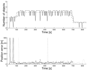
(a) $p_{FN}=0.1$

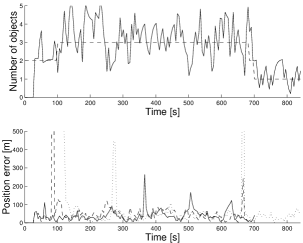
(b) $p_{FN}=0.5$

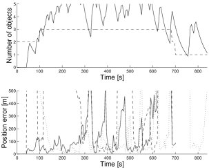
(c) $p_{FN}=0.9$

Figure 1: Tracking errors for the PHD filter. (a) Observation probability 0.9. (b) Observation probability 0.5. (c) Observation probability 0.1. The upper graph in each subfigure shows estimated (solid line) number of targets, compared to the true (dashed line) number. The lower graph shows position errors for the three vehicles. Solid, dashed and dotted lines denote different vehicles. The dotted target appears after 101 s, the dashed target disappears after 687 s and the solid target after 702 s. Position error is measured as the Euclidean distance from the true target position to the nearest detected maxima in the estimated PHD.

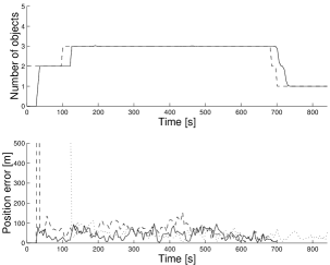
(a) $p_{FN}=0.1$

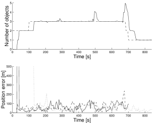
(b) $p_{FN}=0.5$

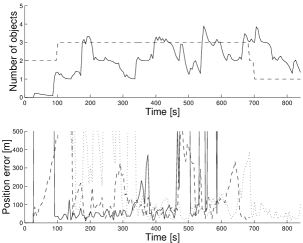
(c) $p_{FN}=0.9$

Figure 2: Tracking errors for the full random set filter, on the same scenario. (a) Observation probability 0.9. (b) Observation probability 0.5. (c) Observation probability 0.1. A complete description of this simulation can be found in [17].

Using the settings described above experiments were performed to test the performance of the PHD particle filter (Figure 1) and to compare it with a particle implementation [17, 18] of the FISST filter [11], which maintains the joint distribution over the full random set over time (Figure 2). $\mathcal{N}=1000$ particles were used to represent a pdf in the PHD filter. The settings of the FISST particle filter simulation can be found in [17].

The tracking performance was measured in two ways, comparing the estimated number of targets with the true value, and measuring the Euclidean distance between the ground truth target positions and the local maxima in the PHD (Section 4).

Both filters were implemented in Matlab, which is a language not suited for real-time applications. However, it should be noted that both algorithms required less or marginally more time than the span of a time-step in the simulation, 5 s, running in Linux on an ordinary desktop computer. This indicates the usability of both algorithms for real-time applications.

One iteration in the FISST particle filter required 4.9 s on average, while an iteration in the PHD particle filter required 0.38 s. The generation of the (discretized) PHD and the fitting of the mixture of Gaussians to the PHD were identical in the two filters, and required 1.2 s on average. Thus one time-step in the full FISST particle filter takes approximately 12 times longer than the corresponding iteration in the PHD filter. This should be kept in mind while comparing the performance of the two filters.

As expected, the FISST particle filter outperforms the PHD particle filter in estimating the number of targets (upper graph in each subfigure) for all tested values of $p_{FN}$. If this is an important aspect of the tracking, a filter maintaining belief over the full random set should be used.

However, the accuracy in position estimation is very similar between the two filters. With high or moderate observation probability (Figures 1a,b and 2a,b), both filters maintain track of all targets, save for a few mistakes in the PHD filter that are quickly recovered from. With a low observation probability, both filters (Figure 1c and 2c) fail to track the targets to a high degree. The reasons for that is simply that the SNR is too low [13, 17].

To conclude, the PHD particle filter’s accuracy in estimating the number of targets is low, and falls quickly with the SNR. However, the positions of the targets are estimated with the same accuracy as provided by a filter representing the full random set.

Thus, the PHD particle filter is a robust and computationally inexpensive alternative to representing the full joint distribution over the random set, when estimation of the number of targets is not the primary issue.

7 Conclusions

The contribution of this paper has been a particle filtering implementation of the PHD filter presented by Mahler and Zajic [12, 13]. The PHD particle filter was applied to tracking of an unknown and changing number of vehicles in terrain, a problem incorporating highly non-linear motion, due to the terrain.

Experiments showed the PHD particle filter to be a fast and robust alternative to a filter where the full joint distribution over the set of targets was maintained over time.

7.1 Future work

This work could be extended along several avenues of research. Firstly, the effects of all parameter settings on the tracking need to be investigated. In the experiments in Section 6, only the degree of missing observations, $p_{FN}$, was varied.

Furthermore, it would be interesting to investigate more sophisticated observation models. The experiments here show clearly that the performance of the filter is strongly dependent on the SNR. One way to heighten the SNR with our type of sensors, human observers, is to take negative information (i.e. absence of reports) into regard. This is possible if the fields of view of the observers are known.

Finally, a real-time implementation should be made, and the filter should be tested over longer time periods with more targets. A larger testbed is currently developed for this purpose.

References

- [1] D. J. Ballantyne, H. Y. Chan, and M. A. Kouritzin. A branching particle-based nonlinear filter for multi-target tracking. In International Conference on Information Fusion, volume 1, pages WeA2:3–10, 2001.
- [2] A. Doucet, N. de Freitas, and N. Gordon, editors. Sequential Monte Carlo Methods in Practice. Springer Verlag, NEw York, NY, USA, 2001.
- [3] T. E. Fortmann, Y. Bar-Shalom, and M. Scheffe. Sonar tracking of multiple targets using joint probabilistic data association. IEEE Journal of Oceanic Engineering, OE-8(3):173–184, 1983.
- [4] I. R. Goodman, R. P. S. Mahler, and H. T. Nguyen. Mathematics of Data Fusion. Kluwer Academic Publishers, Dordrecht, Netherlands, 1997.
- [5] N. Gordon, D. Salmond, and A. Smith. A novel approach to nonlinear/non-Gaussian Bayesian state estimation. IEE Proceedings on Radar, Sonar and Navigation, 140(2):107–113, 1993.
- [6] C. Hue, J-P. Le Cadre, and P. Pérez. Sequential Monte Carlo methods for multiple target tracking and data fusion. IEEE Transactions on Signal Processing, 50(2):309–325, 2002.
- [7] M. Isard and A. Blake. Condensation – conditional density propagation for visual tracking. International Journal of Computer Vision, 29(1):5–28, 1998.
- [8] M. Isard and J. MacCormick. BraMBLe: A Bayesian multiple-blob tracker. In IEEE International Conference on Computer Vision, ICCV, volume 2, pages 34–41, 2001.
- [9] K. Kastella, C. Kreucher, and M. A. Pagels. Nonlinear filtering for ground target applications. In SPIE Conference on Signal and Data Processing of Small Targets, volume 4048, pages 266–276, 2000.
- [10] C-C. Ke, J. G. Herrero, and J. Llinas. Comparative analysis of alternative ground target tracking techniques. In International Conference on Information Fusion, volume 2, pages WeB5:3–10, 2000.
- [11] R. Mahler. An Introduction to Multisource-Multitarget Statistics and its Applications. Lockheed Martin Technical Monograph, 2000.
- [12] R. Mahler. An extended first-order Bayes filter for force aggregation. In SPIE Conference on Signal and Data Processing of Small Targets, volume 4729, 2002.
- [13] R. Mahler and T. Zajic. Multitarget filtering using a multitarget first-order moment statistic. In SPIE Conference on Signal Processing, Sensor Fusion and Target Recognition, volume 4380, pages 184–195, 2001.
- [14] E. Mazor, A. Averbuch, Y. Bar-Shalom, and J. Dayan. IMM methods in target tracking: A survey. IEEE Transactions on Aerospace and Electronic Systems, 34(1):103–123, 1998.
- [15] S. Musick, K. Kastella, and R. Mahler. A practical implementation of joint multitarget probabilities. In SPIE Conference on Signal Processing, Sensor Fusion and Target Recognition, volume 3374, pages 26–37, 1998.
- [16] D. B. Reid. An algorithm for tracking mulitple targets. IEEE Transactions on Automatic Control, AC-24(6):843–854, 1979.
- [17] H. Sidenbladh. Withheld, currently in double-blind review. In IEEE Workshop on Multi-Object Tracking, 2003, submitted.
- [18] H. Sidenbladh and S-L. Wirkander. Particle filtering for random sets. IEEE Transactions on Signal Processing, submitted.
- [19] E. P. Sodtke and J. Llinas. Terrain based tracking using position sensors. In International Conference on Information Fusion, volume 2, pages ThB1:27–32, 2001.
- [20] L. D. Stone. A Bayesian approach to multiple-target tracking. In D. L. Hall and J. Llinas, editors, Handbook of Multisensor Data Fusion, 2002.