Kalman-filtering using local interactions

Abstract

There is a growing interest in using Kalman-filter models for brain modelling. In turn, it is of considerable importance to represent Kalman-filter in connectionist forms with local Hebbian learning rules. To our best knowledge, Kalman-filter has not been given such local representation. It seems that the main obstacle is the dynamic adaptation of the Kalman-gain. Here, a connectionist representation is presented, which is derived by means of the recursive prediction error method. We show that this method gives rise to attractive local learning rules and can adapt the Kalman-gain.

1 Introduction

Linear dynamical systems (LDS) are well studied and widely applied tools in both state estimation and control. Inference in LDS becomes simple, unbiased and has minimized covariance if the Kalman-filter recursion is used. Recently, there is growing interest in Kalman-filters or Kalman-filter like structures as models for neurobiological substrates. It has been suggested that Kalman-filtering (i) may occur at sensory processing ([1, 2]), (ii) may be the underlying computation of the hippocampus ([3]), and may be the underlying principle in control architectures ([4]). Detailed architectural similarities between Kalman-filter and the entorhinal-hippocampal loop as well as between Kalman-filters and the neocortical hierarchy have been described recently ([5, 6]). Interplay between the dynamics of Kalman-filter-like architectures and learning of parameters of neuronal networks has promising aspects for explaining known and puzzling phenomena, such as priming, repetition suppression and categorization ([7, 8]).

Kalman-filter is an on-line recursive algorithm. Unfortunately, Kalman-filtering requires the computation of the Kalman-gain. Recursions of the Kalman-gain matrix assume that covariance matrices of measurement noise and observation noise are known. In general, these parameter sets are not known in advance and may be subject to temporal changes. Moreover, to determine the Kalman-gain, the algorithm requires the inversion of matrices, which is hard to interpret in neurobiological terms. To our best knowledge, all suggested networks computed the Kalman-gain matrix directly, e.g., using matrix inversions.

Here, an alternative route, the recursive prediction error (RPE) method ([9]) is followed. Using this method, we were able to construct a special parametrization, which is (i) on-line and recursive and (ii) makes use of local interactions to estimate the filtering parameters, including the Kalman-gain. The next section (Section 2) reviews background materials, such as the constraints on connectionist systems (Section 2.1), the well known Kalman-filer recursion (Section 2.2). In Section 2.3 the recursive prediction error method is applied to estimate the Kalman-gain. Our particular parametrization and the corresponding architecture are provided in Section 3 and Section 3.1, respectively. Conclusions are drawn in the last section (Section 4). Detailed mapping to the neural substrate is not aimed here: There should be large differences if the goal is the mapping (i) to the control system of the brain, (ii) to the hippocampus, (iii) to the hippocampal-entorhinal loop, or, (iv) to the neocortical layers, etc. All suggestions on Kalman-filtering need to map a connectionist architecture to a part of the brain.

2 Background

2.1 Constraints on connectionist systems

Connectionist systems are special non-linear systems having graph like structures. Nodes of the graph are called neurons, whereas directed edges are the connections. Figure 1 depicts a neuron subject to local interactions. An interaction is called local if it is exerted by a directed connection. The targeted neuron is the subject of the interaction. The end of the directed connection is depicted by a small circle, called synapse. This synapse could be of three types here, it is either excitatory, inhibitory or of multiplying type. The first two of these types are widely considered as neuronal operations. Multiplying type synapse is, however, also possible: a neuron may affect another neuron by modulating the ‘gain’ of that neuron in a multiplicative way ([10]). For a review on different processing capabilities of single neurons, see, e.g., [11]).

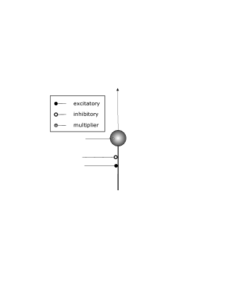
Figure 1: Local interactions of neurons
The node (or neuron) is depicted by the large grey circle. Connections to and from other neurons are depicted by lines, these are called directed connections. The direction of a connection is denoted either by an arrow or by a small circle. The small circle is the synapse of the connection at around the targeted neuron. The interaction (i.e., the connection) targets that neuron, which (i) is in the direction of the arrow, or (ii) is at the circle, or (iii) is targeted by a connection being targeted by the small circle, and so on. The synapse could be of two basic types here, it is either additive or multiplying type. An additive synapse can be either excitatory or inhibitory. We assume that only the excitatory synapses can be adapted. At the same time, we also assume that feedforward inhibition, which is always present ([12]), plays a role and learning occurs relative to a negative background. In turn, feedforward inhibitory synapses – which are not shown in our figures – and adapting excitatory synapses may exert an effective inhibition. That is, matrices representing excitatory synapse sets may have negative elements.

From the point of view of neuronal modelling,

1. the series of observations constitute the input to the model,

2. the learning task corresponds to finding the best parametrization and the best hidden variables given all past observations and subject to constraints prescribed by the norm (the measure) of a model and the noise of assumed by this model, whereas

3. filtering corresponds to the estimation of the hidden variables given the past observations.

The seminal work of Hebb ([13]) was a brilliant first attempt in its time to link neurophysiology with higher order behavioral phenomena studied by psychology. The central thesis postulated that changes in synaptic connection strength is primarily based on the correlation between the pre- and postsynaptic neural activities. Recent experiments ([14, 15, 16], for a review, see, e.g., [17]) revealed, however, that exact timing and temporal dynamics of the neural activities play a crucial role in forming the neuronal base of plasticity. The novel concept to generally describe the modified variants of the original form of Hebbian learning is called spike-time dependent synaptic plasticity (STDP). The term ‘spike’ denotes the fast potential change which propagates over the neurons and induces synaptic neurotransmitter release, which, in turn, may result in synaptic modifications. STDP means that strengthening occurs (i) if the neuron fires and (ii) if the excitatory synapse targeting this neuron delivered a spike within a narrow time window around the time of firing. On the other hand, weakening occurs if the delivered spike at the excitatory synapse is outside of this short time window.

2.2 Kalman-filter recursion

Let us consider the following linear dynamical system (LDS):

$$\mathbf{y}_{t} = \mathbf{H}\mathbf{x}_{t}+\mathbf{n}_{t}\text{ observation process}$$ (2.1)

$$\mathbf{x}_{t+1} = \mathbf{F}\mathbf{x}_{t}+\mathbf{m}_{t}\text{ dynamics of hidden variables}$$ (2.2)

where $\mathbf{m}_{t}\propto\mathcal{N}(0,\Pi)$, $\mathbf{n}_{t}\propto\mathcal{N}(0,\Sigma)$ are independent noise processes. Here, notation $\mathcal{N}(\mathbf{m},\Sigma)$ is a shorthand to denote a stochastic variable of expectation value $\mathbf{m}$ and covariance matrix $\Sigma$. Our task is the estimation of

hidden variables $\mathbf{x}(t)\in\mathbf{R}^{n}$ given the series of observations $\mathbf{y}(\tau)\in\mathbf{R}^{p}$, $\tau\leq t$.

For estimations in squared (Euclidean) norm and Gaussian noise, the optimal solution was derived by Rudolf Kalman ([18, 19]). The Kalman-filter recursion is reproduced here: Let $E$ and $Cov$ denote the expectation value and the covariance matrix operators, respectively. Let us introduce the following notations: $\hat{\mathbf{x}}(t|\tau)=E(\mathbf{x}_{t}|\mathbf{y}_{1},\ldots\mathbf{y}_{\tau})$, $\mathbf{N}_{t}=Cov(\mathbf{x}_{t}|\mathbf{y}_{1},\ldots\mathbf{y}_{t})$, and $\mathbf{M}_{t}=Cov(\mathbf{x}_{t}|\mathbf{y}_{1},\ldots\mathbf{y}_{t-1})$

Lemma 1 (Kalman-filter recursion)

Assume that $\hat{\mathbf{x}}(t-1|t-1)$,$\mathbf{N}_{t-1}$ has been determined. Then

$$\hat{\mathbf{x}}(t|t-1) = \mathbf{F}\hat{\mathbf{x}}(t-1|t-1)$$ (2.3)

$$\mathbf{M}_{t} = \mathbf{F}\mathbf{N}_{t-1}\mathbf{F}^{T}+\Pi$$ (2.4)

$$\mathbf{K}_{t}^{f} = \mathbf{M}_{t}\mathbf{H}^{T}(\mathbf{H}\mathbf{M}_{t}\mathbf{H}^{T}+\Sigma)^{-1}$$ (2.5)

$$\hat{\mathbf{x}}(t|t) = \hat{\mathbf{x}}(t|t-1)+\mathbf{K}_{t}^{f}\big{(}\mathbf{y}_{t}-\mathbf{H}\mathbf{F}\hat{\mathbf{x}}(t-1|t-1)\big{)}$$ (2.6)

$$\mathbf{N}_{t} = (\mathbf{I}-\mathbf{K}_{t}^{f}\mathbf{H})\mathbf{M}_{t}$$ (2.7)

where $\mathbf{I}$ denotes the identity transformation (i.e., the identity matrix) and superscript $T$ denotes transposition.

Combining equations 2.3 and 2.6, the following filter-equation emerges:

$$\hat{\mathbf{x}}(t+1|t+1) =\underbrace{\mathbf{F}\hat{\mathbf{x}}(t|t)}_{\hat{\mathbf{x}}(t+1|t)}+\mathbf{K}_{t+1}^{f}\big{(}\mathbf{y}_{t+1}-\mathbf{H}\mathbf{F}\hat{\mathbf{x}}(t|t)\big{)}$$ (2.8)

One may also introduce the so called prediction equation:

$$\hat{\mathbf{x}}(t+1|t) =\mathbf{F}\hat{\mathbf{x}}(t|t-1)+\mathbf{K}_{t}^{p}\big{(}\mathbf{y}_{t}-\mathbf{H}\hat{\mathbf{x}}(t|t-1)\big{)}=\mathbf{F}\hat{\mathbf{x}}(t|t)$$ (2.9)

where $\mathbf{K}^{p}_{t}=\mathbf{F}\mathbf{K}_{t}^{f}$, which can be used to make an estimation before the $(t+1)$th measurement.

In the literature, the two different quantities, i.e., $\mathbf{K}_{t}^{f}$ (Eq. 2.5) and $\mathbf{F}\mathbf{K}_{t}^{f}$ (Eq. 2.9) are both called Kalman-gains.

2.3 Review of the recursive prediction error method

Here, we shall consider the filtering task and the learning task. This latter will be restricted to the learning of parameters required for proper adjustment of the Kalman-gain.

Let us make the following notes. Iterations of $\mathbf{K}_{t}^{f}$, $\mathbf{K}_{t}^{p}$, $\mathbf{M}_{t}$, and $\mathbf{N}_{t}$ are independent from measurements on $\mathbf{y}_{1},\ldots\mathbf{y}_{t}$. However, these quantities depend from quantities $\{\mathbf{H},\mathbf{F},\Sigma$ and $\Pi\}$. The dependencies, at first sight, do not seem to admit a neuronal form. The problem is in the computation of the Kalman-gain (Eq. 2.5): this equation includes a matrix inversion, which does not admit a connectionist (i.e., artificial neuronal) network form. Moreover, it seems unlikely, that previous knowledge of covariance matrices $\Sigma$ and $\Pi$ can be assumed for neuronal systems.

In the procedure that follows, we shall assume that the Kalman-gain constitutes the unknown parameter of the system. The Kalman-gain will be estimated on-line using the measured values of $\mathbf{y}_{t}$ (i.e., the input of the neuronal architecture). Because an on-line estimation makes use of (i) the estimated parameters, (ii) the optimization of the activities given the actual observations, and (iii) updates the estimated parameters given the optimized activities and the previous estimations, on-line methods are best suited to changing world. The price is that on-line estimation may not be optimal for all past observation (this is not desirable in a changing world, anyway). Instead, on-line estimation becomes optimal asymptotically. It is well known that under rather mild conditions, both Kalman-gains, i.e., $\mathbf{K}_{t}^{p}$ ,$\mathbf{K}_{t}^{f}$ converge with exponential speed to the asymptotic $\mathbf{K}^{p}$ and $\mathbf{K}^{f}$ values, respectively (i.e., $\lim_{t}\mathbf{K}_{t}=\mathbf{K}$). In turn, on-line estimation is an attractive alternative when the goal is the estimation of the parameter(s) of the Kalman-gain. We shall substitute equations 2.3-2.7 by the on-line methods. We shall apply the recursive prediction error method ([9]) to derive recursive estimation for the Kalman-gain.

Let $\mathbf{K}=\mathbf{K}(\theta)$ denote the parametrization of $\mathbf{K}$, where $\mathbf{K}(\theta)$ may depend on $\theta$ arbitrarily. We shall use this freedom to choose a particular form of the dependence. Now, our task is to estimate $\theta$ and then to compute $\mathbf{K}(\theta)$ using the estimated value of $\theta$. For the sake of simplicity, variable $\theta$ will be scalar in the derivation below. The same derivation follows for vector and matrix variables. Also, derivation concerns the estimation of matrix $\mathbf{K}^{p}_{t}$, but similar derivation can be provided for matrix $\mathbf{K}^{f}_{t}$.

First, the prediction equation (Eq. 2.9) shall be investigated. Let $\hat{\mathbf{x}}(t,\theta)$ denote the predictive estimation of the hidden variables belonging to $\theta$. Equation 2.9 can be written as

$$\hat{\mathbf{x}}(t+1,\theta) = \mathbf{F}\hat{\mathbf{x}}(t,\theta)+\mathbf{K}^{p}(\theta)(\mathbf{y}(t)-\mathbf{H}\hat{\mathbf{x}}(t,\theta))$$ (2.10)

The goal is to find the value of $\theta$ that minimizes the squared norm of the reconstruction error vector, which is defined as $\epsilon(t,\theta)=\mathbf{y}(t)-\mathbf{H}\hat{\mathbf{x}}(t,\theta)$. Vector $\mathbf{H}\hat{\mathbf{x}}(t,\theta)$, which is derived from the hidden variables and should match the input in squared norm, will be called the reconstructed input. By definition, the reconstruction error vector is a stochastic variable with zero mean and $\Lambda$ covariance matrix ($\mathcal{N}(0,\Lambda)$). For the purpose of on-line estimation, the $\Lambda$ covariance matrix needs to be estimated from the data. The said goal, in mathematical terms, has the following form:

$$V(\theta)=E\left(\epsilon(t,\theta)^{T}\Lambda^{-1}\epsilon(t,\theta)\right)\,\,\rightarrow\,\,\min_{\theta}$$ (2.11)

Equation 2.11 can be seen as a maximum likelihood problem. We shall apply the following procedure: (i) The expectation value will be estimated by sample averaging, i.e., stochastic gradient approximation will be used. (ii) $\theta$ will be minimized along the gradient. Let us make use of the notation: $\mathbf{w}(t,\theta)=\frac{\partial}{\partial\theta}\hat{\mathbf{x}}(t,\theta)$ and let $\hat{\mathbf{y}}(t,\theta)=\mathbf{H}\hat{\mathbf{x}}(t,\theta)$ denote the reconstructed input. Minimization of Eq. 2.11 leads to: $\hat{\theta}(t)=\hat{\theta}(t-1)+\gamma(t)\mathbf{v}(t)^{T}\Lambda^{-1}\epsilon(t)$, where $\gamma(t)>0$ is the learning rate, shorthand $\mathbf{v}(t,\theta)$ is given as $\mathbf{v}(t,\theta)=\frac{\partial}{\partial\theta}(\hat{\mathbf{y}}(t,\theta)-\mathbf{y}(t))$ and a recursive equation can be derived for $\mathbf{w}(t+1,\theta)$ from Eq. 2.10 if it is differentiated according to $\theta$. The following recursive estimation can be gained for the Kalman-gain matrix $\mathbf{K}$:

Lemma 2 (Local Kalman-filter recursion)

Assume that $\hat{\mathbf{x}}(t)$, $\hat{\mathbf{w}}(t)$, $\hat{\theta}(t)$, $\hat{\Lambda}^{-1}(t)$ are given. Then

$$\hat{\mathbf{y}}(t) = \mathbf{H}\hat{\mathbf{x}}(t)$$ (2.12)

$$\epsilon(t) = \mathbf{y}(t)-\hat{\mathbf{y}}(t)$$ (2.13)

$$\hat{\mathbf{x}}(t+1) = \mathbf{F}\hat{\mathbf{x}}(t)+\mathbf{K}(\hat{\theta}(t))\epsilon(t)$$ (2.14)

$$\hat{\mathbf{v}}(t) = \mathbf{H}\hat{\mathbf{w}}(t)$$ (2.15)

$$\hat{\mathbf{w}}(t+1) = \mathbf{F}\hat{\mathbf{w}}(t)+\mathbf{K}^{\prime}(\hat{\theta}(t))\epsilon(t)-\mathbf{K}(\hat{\theta}(t))\hat{\mathbf{v}}(t)$$ (2.16)

$$\hat{\theta}(t+1) = \hat{\theta}(t)+\gamma(t)\hat{\mathbf{v}}^{T}(t)\hat{\Lambda}^{-1}(t)\epsilon(t)$$ (2.17)

$$\hat{\Lambda}(t+1) = \hat{\Lambda}(t)+\gamma(t)\left[\epsilon(t)\epsilon(t)^{T}-\hat{\Lambda}(t)\right]$$ (2.18)

where $\mathbf{K}^{\prime}$ denotes $\frac{\partial K}{\partial\theta}$. The auxiliary vector $\mathbf{w}$, which can be derived from the hidden vector $\hat{\mathbf{x}}$ by differentiation according to $\theta$, will play a crucial role in providing neuronal representation. For later purposes, we rewrite Eq. 2.18 into the following stable form:

$$\hat{\Lambda}^{-1}(t+1) = \hat{\Lambda}^{-1}(t)+\gamma(t)\left[\hat{\Lambda}^{-1}(t)-\left(\hat{\Lambda}^{-1}(t)\epsilon(t)\right)\left(\hat{\Lambda}^{-1}(t)\epsilon(t)\right)^{T}\right]$$ (2.19)

In both recursions, i.e., in Eq. 2.18 and in Eq. 2.19, matrix $\hat{\Lambda}$ is an estimation of the covariance matrix of the reconstruction error vector $\epsilon$. In recursion Eq. 2.19, the inverse of the correlation matrix is estimated directly. Update Eq. 2.18 is a signal-Hebbian learning rule. Update Eq. 2.19 is in different form and can be seen as a neural update if spike-time dependent synaptic plasticity is taken into account, as it will be described later.

3 Local Kalman-filter

Now, let us choose an element of matrix $\mathbf{K}$, say $\mathbf{K}_{ij}$. In what follows, we shall make the particular assumption that $\mathbf{K}_{ij}$ is an exponential function of $\theta$. This assumption allows us to simplify the architecture considerably. The simplification is warranted by the particular property of the exponential dependence that $\mathbf{K}^{\prime}_{ij}=\mathbf{K}_{ij}$, which will be important when the local connectionist architecture will be presented: We can use matrix $\mathbf{K}$ for both purposes, i.e., for $\mathbf{K}$ itself and for $\mathbf{K}^{\prime}$. In our formulation, the recursive correction of the Kalman-gain assumes the multiplying exponentiated gradient form ([20, 21]):

$$\mathbf{K}_{ij}(\theta(t+1)) = \exp\left(\gamma(t)\hat{\mathbf{v}}(t)\hat{\Lambda}^{-1}(t)\epsilon(t)\right)\,\mathbf{K}_{ij}(\theta(t))$$ (3.1)

Now, Eq. 2.16 can be written as

$$\hat{\mathbf{w}}(t+1) = \mathbf{F}\hat{\mathbf{w}}(t)+\mathbf{K}(\hat{\theta}(t))\left(\epsilon(t)-\hat{\mathbf{v}}(t)\right)$$ (3.2)

$$= \mathbf{F}\hat{\mathbf{w}}(t)+\mathbf{K}(\hat{\theta}(t))\left(\epsilon(t)-(\mathbf{H}\hat{\mathbf{w}}(t))\right)$$ (3.3)

$$= \mathbf{K}(\hat{\theta}(t))\epsilon(t)+\left(\mathbf{F}-\mathbf{K}(\hat{\theta}(t))\mathbf{H}\right)\hat{\mathbf{w}}(t)$$ (3.4)

3.1 Architecture

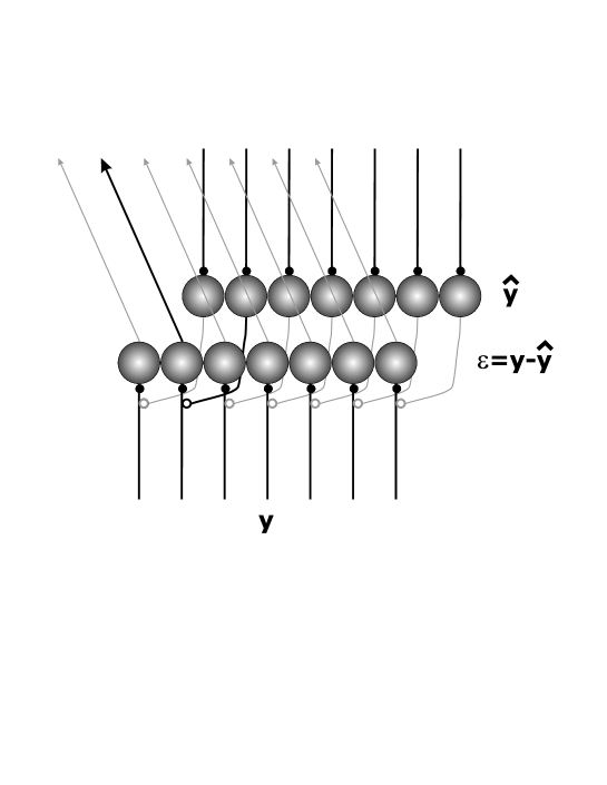
Figure 2: Computation of reconstruction error $\epsilon$
Difference between two vector quantities can be computed by an ordered array of connections of inhibitory type.

The reconstruction error vector ($\epsilon$) is computed by differencing between the input ($\mathbf{y}$) and the estimated input $\hat{\mathbf{y}}$. The circuitry is shown in Fig. 2.

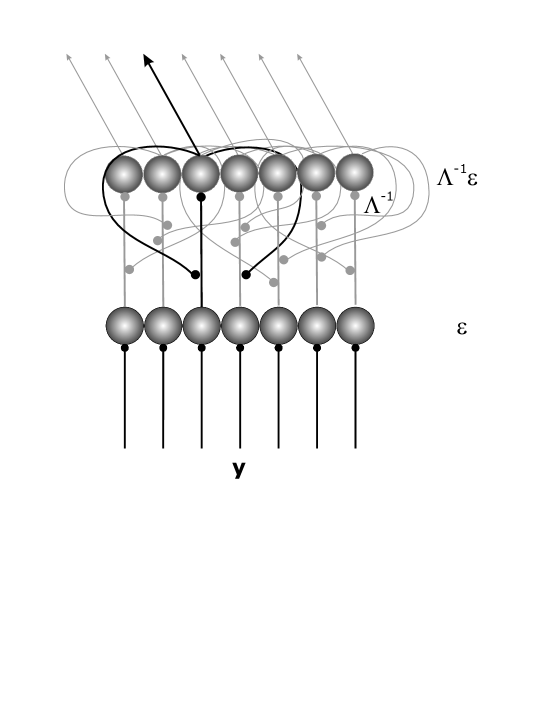
Figure 3: Learning and multiplying by the inverse of correlation matrix $\Lambda$
There is a recurrent collateral system (a full connectivity excitatory feedback structure) at the output layer. (Only few connections are shown.) Noise is present and accidental coincidences between excitatory inputs and neuronal firing can give rise to self-strengthening proportional to the connection strength [5]. This effect provides the first (positive) term of Eq. 2.19. We assume that the recurrent collaterals have considerable delays and taht synapses are weakened because of the spike-time dependent synaptic plasticity process. The weakening effect is proportional to the postsynaptic activities and to the activities carried by the recurrent collaterals: This effect provides the negative term of Eq. 2.19. In turn, the architecture executes the update of Eq. 2.19 and multiplies the input (i.e., $\epsilon$) by $\Lambda^{-1}$. For details, see text.

Computation of the parameter $\theta$ of the Kalman-gain can be performed by computing vector $\Lambda^{-1}\epsilon$. To this end, vector $\epsilon$ is to be multiplied by the inverse of the correlation matrix $\Lambda$ of the $\epsilon$ vectors themselves. Matrix $\Lambda$ is to be learned by the RPE method.

Learning can be accomplished by Hebbian means as depicted in Fig. 3: The reconstruction error layer provides input for an auxiliary neural sub-layer. This layer will output vector $\Lambda^{-1}\epsilon$. There is a full connectivity excitatory feedback structure at this sub-layer. It is assumed that noise is present in the system and that this noise gives rise to self-strengthening for all feedback connections. This self-strengthening effect is assumed to be proportional to the connection strength, i.e., it is responsible for the first (positive) term of Eq. 2.19. It is assumed, too, that this feedback structure, called recurrent collaterals have considerable delays, feedback arrives to the excitatory synapses late and weakening of the synapses occur because of the STDP process. The weakening is proportional to the postsynaptic activity and to the activity carried by the recurrent collateral and, in turn, the negative term of Eq. 2.19 emerges. The emerging full update corresponds to Eq. 2.19.

For proper outputs, however, an additional structure is required: The excitatory feedback effect should act only once. We assume that an augmenting set of inhibitory neurons exist (these are not shown in Fig. 3) and that these inhibitory neurons are excited by the same auxiliary neural sub-layer. Moreover, it is assumed that connections originated by the inhibitory neurons target the feedback excitatory synapses of the auxiliary neural sub-layer. The extra step to excite an inhibitory layer makes the inhibitory effect delayed relative to the excitatory effect at the feedback excitatory synapses. Inhibition stops the excitatory effect and excitatory feedback can occur only once in each iteration step. It is intriguing that this complex excitatory-inhibitory structure does exist in the cortex ([22]). It then follows that (i) the circuitry of Fig. 3 performs the RPE computation prescribed by Eq. 2.19 and that the output of the sub-layer is equal to $\Lambda^{-1}\epsilon$.

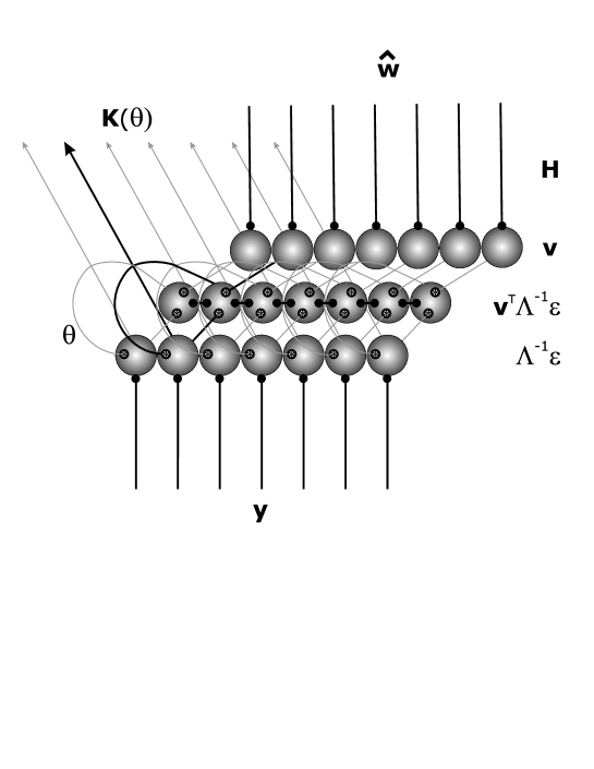
Figure 4: Computation and influence of parameter $\theta$, the parameter of the Kalman-gain
Component-by-component multiplication of vector $\mathbf{v}$ (Eq. 2.15) and vector $\Lambda^{-1}\epsilon$ are performed and the components are summed up in a separate sub-layer. The output of this layer influences the Kalman-gain via synapses of multiplying types. These synapses influence the outputs of neurons of the reconstruction error vector.

Last, the parameter of the Kalman-gain is to be computed. The computation is made of three parts. First, vector $\mathbf{v}$ (Eq. 2.15) and vector $\Lambda^{-1}\epsilon$ are to be multiplied component-by component. Then the individual terms need to sum up to correct the previous estimation of the parameter of the Kalman-gain. Finally, the re-estimated parameter influences each outgoing connections in a uniform but non-linear fashion. This non-linear dynamic effect is the attenuation process of the Kalman-filter, i.e., the tuning of the Kalman-gain. We made the assumption that this non-linear influence is, in fact, exponential. The corresponding circuitry is shown in Fig. 4. Although, here a connectionist model is constructed, still, it may be important to emphasize that the Kalman-gain influences the output of the reconstruction error layer in a uniform fashion. It is then possible that not a full layer, but a single (or a few) neuron(s) (i) compute the scalar product of vectors $\mathbf{v}$ and $\Lambda^{-1}\epsilon$ and (ii) target the neurons of the reconstruction error layer to tune the Kalman-gain as required for Kalman-filtering.

The distinct parts of the RPE computation can be made recursive by means of a loop architecture. The loop architecture is depicted in Fig. 5.

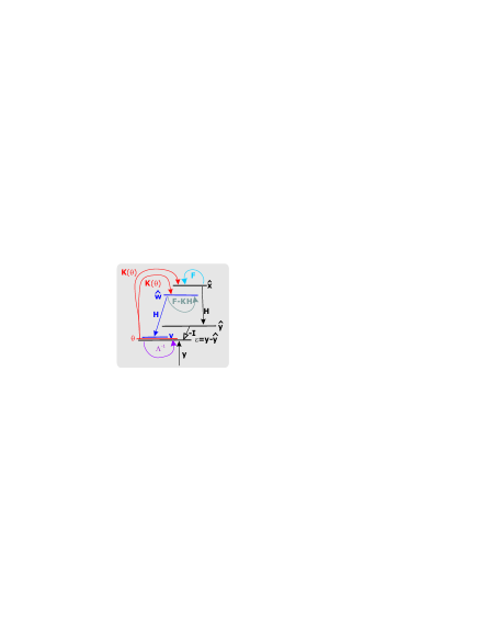
Figure 5: Architecture to execute the recursive prediction error method
The exponentiated dependence on the parameter of the Kalman-gain allows for a simple loop structure. The computations of Figs. 2-4 together, perform Kalman-filtering in the depicted loop as prescribed by Eqs. 2.12-3.4. Solid arrows: excitatory connections. Empty arrow: inhibitory connections. Recursive prediction error method proceeds as follows: Neural activities are given at time $t$ at each layer. To compute the estimation at time $t+1$, all activities are propagated through the connections represented by the arrows of the figure, simultaneously. Emerging constraints are as follows: (i) There should be an associative matrix connecting components of the estimation of the hidden variables and this matrix should be equal to $\mathbf{F}$. (ii) There should also be an associative matrix connecting components of the estimation of auxiliary vector $\mathbf{w}$ and this matrix should be equal to $\mathbf{F}-\mathbf{K}\mathbf{H}$.

Figures 2-5 demonstrate that Kalman-filtering can be performed by local means in a loop through the RPE method. This observation supports top-down modelling efforts, which have appeared recently in the literature ([1, 2, 3, 5, 6, 4]). The top-down modelling suggestion – that Kalman-filtering may play a role in cortical computations – calls for reinforcement from the bottom-up modelling methods of computational neuroscience. Our work makes a step towards this direction; we have transformed the suggestions of top-down modelling into a dynamical neural architecture with appealing Hebbian learning rules. The particular form of Kalman-filtering we presented here poses several questions. We list a few of them. (i) How can be this architecture mapped onto the neocortex? (ii) How can be the derived computations performed in the neural substrate? (iii) In particular, how reasonable is our assumption that the Kalman-gain exponentially depends on its parameter? These questions, which can be seen as the predictions of our model, remain open and call for further studies.

4 Conclusions

In this paper we have presented a neural (connectionist) representation for Kalman-filtering. The issue is worth to consider given the recent advances in the literature ([2, 6, 4]). Regarding the cited works we feel that all have the problem in common: Kalman-filtering should be given a local connectionist architecture for the proposed top-down approaches. Here, we have shown that yes, connectionist representation is possible for Kalman-filtering: The recursive prediction error method suits the requirements imposed by Hebbian constraints. Moreover, RPE provides an appealing on-line learning scheme. This is a promising start. However, the mapping of the architecture to neocortical areas and the question if the predictive matrices of the Kalman-filter could be learned by Hebbian means remained open. Also, further studies starting from parameters of the neuronal substrate are in need to explore the particular predictions of the RPE model of Kalman-filtering.

References

- [1] R. Rao, D. Ballard, Dynamic model of visual recognition predicts neural response properties in the visual cortex, Neural Comput 9 (1997) 721–763.
- [2] R. Rao, D. Ballard, Predictive coding in the visual cortex: A functional interpretation of some extra-classical receptive-field effects, Nature Neuroscience 2 (1999) 79–87.
- [3] O. Bousquet, K. Balakrishnan, V. Honavar, Proceedings of the Pacific Symposium on Biocomputing, 1999, Ch. Is the Hippocampus a Kalman Filter?, pp. 619–630.
- [4] E. Todorov, M. Jordan, Optimal feedback control as a theory of motor coordination, Nature Neuroscience 5 (2002) 1226–1235.
- [5] A. Lőrincz, G. Buzsáki, The parahippocampal region: Implications for neurological and psychiatric dieseases, in: H. Scharfman, M. Witter, R. Schwarz (Eds.), Annals of the New York Academy of Sciences, Vol. 911, New York Academy of Sciences, New York, 2000, Ch. Two–phase computational model training long–term memories in the entorhinal–hippocampal region, pp. 83–111.
- [6] A. Lőrincz, B. Szatmáry, G. Szirtes, Mystery of structure and function of sensory processing areas of the neocortex: A resolution, J. Comp. Neurosci. 13 (2002) 187 205.
- [7] A. Lőrincz, G. Szirtes, B. Takács, I. Biederman, R. Vogels, Relating priming and repetition suppression, Int. J. of Neural Systems 12 (2002) 187–202.
- [8] S. Kéri, G. Benedek, Z. Janka, P. Aszalós, B. Szatmáry, G. Szirtes, A. Lőrincz, Categories, prototypes and memory systems in alzheimer’s disease, Trends in Cognitive Science 6 (2002) 132–136.
- [9] L. Ljung, T. Soderstrom, Theory and practice of recursive identification, MIT Press, Cambridge, MA, 1993.
- [10] E. Salinas, P. Thier, Gain modulation: a major computational principle of the central nervous system., Neuron 27 (2000) 15–21.
- [11] C. Koch, I. Segev, The role of single neurons in information processing, Nature Neuroscience 3 (2000) 1171–1177.
- [12] G. Buzsáki, Feed-forward inhibition in the hippocampal formation, Prog. Neurobiol. 22 (1984) 131–153.
- [13] D. Hebb, The Organization of Behavior: A Neuropsychological Theory, Wiley, New York, 1949.
- [14] H. Markram, J. Lubke, M. Frotscher, B. Sakmann, Regulation of synaptic efficacy by coincidence of postsynaptic APs and EPSPs, Science 215 (1997) 213–215.
- [15] J. Magee, D. Johnston, A synaptically controlled, associative signal for hebbian plasticity in hippocampal neurons, Science 275 (1997) 209–213.
- [16] C. Bell, V. Han, Y. Sugawara, K. Grant, Synaptic plasticity in a cerebellum-like structure depends on temporal order, Nature 387 (1997) 278–281.
- [17] L. Abbott, S. Nelson, Synaptic plasticity: taming the beast, Nature Neuroscience 3 (2000) 1178–1183.
- [18] A. Bagchi, Optimal control of stochastic systems, Prentice Hall, New York, 1993.
- [19] R. Elliott, A. Lakhdar, J. Moore, Hidden Markov models. Estimation and control, Springer Verlag, New York, 1995.
- [20] N. Littlestone, P. Long, M. Warmuth, On-line learning of linear functions, Journal of Computational Complexity 5 (1995) 1–23.
- [21] J. Kivinen, M. K. Warmuth, Additive versus exponentiated gradient updates for linear prediction, Information and Computation 5: 1-23, 132 (1997) 1–64.
- [22] T. Freund, G. Buzsáki, Interneurons of the hippocampus, Hippocampus 6 (1996) 345–470.