Data Structure for a Time-Based Bandwidth Reservations Problem
Abstract
We discuss a problem of handling resource reservations. The resource can be reserved for some time, it can be freed or it can be queried what is the largest amount of reserved resource during a time interval. We show that the problem has a lower bound of per operation on average and we give a matching upper bound algorithm. Our solution also solves a dynamic version of the related problems of a prefix sum and a partial sum.
1 Introduction
In Computer Communications we need to make bandwidth reservations over the Internet to provide Quality of Service (QoS) for the end users. The IETF (Internet Engineering Task Force) defined a standard for Integrated Services in routers ([25, 12]) and the end-to-end reservation setup protocol RSVP ([7]). Since the protocol does not scale well ([16]) IETF came up with a new approach, known as differentiated services (diffserv, [5]). Schelén et. al. ([21, 20]) used the diffserv to design a new QoS architecture. In this architecture they provide virtual leased lines using the differentiated services to perform admission control through the system of agents. The agents work on per-hop basis and they need to maintain a database of the reservations made on their hop. In the backbone of the Internet it will most likely be many reservations to administrate and hence the use of an efficient data structure will be required. Moreover, in the design of the agents the authors propose that a single agent administrates several hops to make it more attractive for the ISP’s (Internet Service Provider). Such a scenario even increases the need for use of an efficient data structure. Therefore Schelén et. al. in [19] proposed a solution that was, however, limited to a predefined set of possible time intervals over which the reservation could be made.
The bandwidth reservation problem is a special case of a more generic problem, where we need to administrate a limited resource over the time; e.g. use of human resources, computational power of super-computer, pool of cars etc. Although the solution in this paper covers all these problems, we use the term bandwidth when we talk about the reserved resource.
Definition 0.1
In the bandwidth reservation problem we have a fixed amount of bandwidth to administer. Customers want to make reservations for a part of the bandwidth during a time interval (, the interval starts at time and ends at time , and it includes ). The operations to support, besides initialization and destruction, are:
-
•
, that reserves units of bandwidth for the time period , where .
-
•
, that frees the reserved bandwidth during the interval . Note that freeing the bandwidth is the same as making a reservation with a negative bandwidth.
-
•
, that returns maximum reserved bandwidth during the interval .
For the sake of clarity, we sometimes use the subscripts and for queries and reservations respectively. For example, a reservation interval . In the paper we also use the notation denoting a function returning the bigger of and .
1.1 Literature background
In the literature we could not find any reference to the bandwidth reservation problem with an arbitrary reservation interval – i.e. interval where endpoints are not drawn from a predefined set. However, the problem is similar to problems we find in other fields of computer science that handle intervals on a real line (e.g. computational geometry, dynamic computation and geometric search [18, 3, 9, 10]). These problems are generally solved using segment trees ([22, 17]), which were introduced by Bentley ([4]) as a solution to the Klee’s rectangle problem ([14]). The limitation in all these problems is that the end-points of the intervals belong to a fixed set of points. In our problem we have no such a set.
Kuchem et. al. in ([15]) presented in a way similar data structure to ours, although it still deals with a fixed set of points. They use the structure in a VLSI design. Bose et. al. independently developed in [6] a similar data structure to solve a number of geometric problems.
Another pair of related problems are the well studied partial sum problem ([11], brief in [13]), and the prefix sum problem ([11]). In the prefix sum problem we have an array on which we want to perform these two operations: (1) : ; and (2) : for arbitrary values of , and . In [11] Fredman shows a lower bound of for the problem under the comparison based model. In the same paper Fredman also presents an algorithm with a matching upper bound.
In the rest of the paper we first show that the logarithmic lower bound carries over to the bandwidth reservation problem. We continue with a presentation of a data structure we call BinSeT (binary segment tree) that gives us a matching upper bound. We conclude the paper with final remarks.
2 Lower bound
Theorem 0.1
Given an arbitrary sequence of operations from a bandwidth reservation problem, each of them requires at least comparisons on the average, where is the number of intervals we are dealing with.
Proof: Assume that we have a solution to the bandwidth reservation problem that requires time. We will show how to use such a solution to solve the prefix sum problem in time which contradicts the lower bound by Fredman ([11]).
First, we introduce an extra point right to all other points representing . It is needed since in our problem we are dealing with open intervals on the right side. Next, we translate the array of elements in the prefix sum problem into end-points of intervals. More precisely, the element of the array is represented by the interval that starts at point and ends at the right most point : . Therefore, the reserved bandwidth at point is the sum of all reserved bandwidths for intervals starting at points , where . This gives us the following translation of prefix-sum problem operations:
-
•
the operation into ; and
-
•
the operation into a query .
This translation gives us an solution to the prefix sum problem and hence contradicts the lower bound by Fredman.
Note that, the prefix sum as presented by Fredman ([11]) is also a static problem – i.e. the array of elements neither expands nor shrinks. On the other hand, the solution we present in the following section does support insertion of new points (intervals) and deletion of points (intervals). Hence, by using the translation in the proof we also get a logarithmic solution to the dynamic version of the prefix-sum problem.
3 Upper bound
To prove an upper bound we use a data structure called BinSeT that supports the required operations in logarithmic time. Before going into details of data structure we describe how we represent reservations.
3.1 Representation of reservations
We do not represent a reservation interval as a single entity, but we split it into two, what we call, reservation events. A reservation event is a point in time when an increase or decrease in the amount of a reserved bandwidth occurs. For example, we store a reservation as reservation events and . In other terms, we convert an interval into two semi-infinite intervals and . Hence, the operations from Definition 0.1 are converted:
-
•
into adding of reservation events and ; and
-
•
into adding of reservation events and ; while
-
•
, remains the same.
If we want to store extra information with each reservation we introduce an additional dictionary data structure to store this information and bind the reservation events to records in the dictionary.
3.2 Data Structure
The binary segment tree BinSeT is a data structure that combines properties of a binary and a segment tree. The former permits dynamic insertion and deletion of reservation events and the later answering queries about the maximum reserved bandwidth. In detail, the leaves represent and store information about the reservation events, while each internal node covers a segment (interval) and stores information about the values (bandwidth) on that interval. To ensure worst case performance, we balance BinSeT tree as an AVL tree (cf. [8, 1, 24]) – hence we also need to talk about the height of BinSeT tree. This gives the following invariance for every node of our data structure:
Invariance 0.1
The information stored with the node representing an interval is the maximum value on the interval and the change of the value on the interval. Besides, with a node is also stored the left-most event in the right subtree . The difference of heights of left and right subtree is at most one.
Note, if a node covers interval , the left subtree covers interval and the right subtree the interval .
In simpler terms, in the BinSeT tree each node has its own local system of reserved resource values on its interval. The system is offset to the global so, that in the beginning of the interval the value is considered to be . To get total (global) value of reserved resources one has to add -s for all left siblings on the path from the node to the root.
It is easy to verify the following lemma:
Lemma 0.1
Let be left child and right child of an internal node . Then the equations:
| (1) |
hold for all nodes .
The detail data structure is represented in Algorithm 0.1.
typedef struct _sBinSeT {
tResource ;
tResource ;
tTime ;
unsigned int height;
struct _sBinSeT* left;
struct _sBinSeT* right;
} tBinSeT;
The structure is slightly different from the one described above since it does not include times and , but only the . However, values and can be implicitly calculated during recursive descend. At this point we note two things: first, a node has either two sub-trees (an internal node) or none (a leaf); and second, a leaf stores in both and the amount of the reserved bandwidth at the reservation event it represents, and in the time of the event. As a consequence of the first observation we conclude, that the number of internal nodes is one less than the number of leaves. Since the number of leaves is at most , where is a number of reservation intervals, this proves the following lemma, under the RAM model:
Lemma 0.2
The size of the BinSeT storing reservation events is words.
3.3 Operations
Finally we describe how to implement efficiently queries and adding of reservation events. All our solutions will be recursive and will start traversing the data structure from the root. We assume that we store with BinSeT also the time of the first () and the last () reservation event. These are also times and , respectively, for the root of the complete BinSeT. If we descend in the left subtree, then the and for this subtree become values and , respectively, of the current root. We treat similarly the right subtree. This is also the reason why we need not store values and with a node.
We start with a query (see Algorithm 0.2).
tResource MaxReserved(tBinSet* node, tTime t0, tTime t1, tInterval query) {
tResource leftMax, rightMax;
tInterval queryAux;
if ((t0 == query.t0) && (t1 == query.t1)) /* whole interval – stopping condition */
return node->;
if (query.t1 <= node->) /* query in left subinterval */
return MaxReserved(node->left, t0, node->, query);
if (node-> <= query.t0) /* query in right subinterval */
return node->left-> +
MaxReserved(node->right, node->, t1, query);
queryAux= query; queryAux.t1= node->; /* query in both subinterval – so split it */
leftMax= MaxReserved(node->left, t0, node->, queryAux);
queryAux= query; queryAux.t0= node->;
rightMax= MaxReserved(node->right, node->, t1, queryAux);
return max(leftMax, node->left-> + rightMax);
} /* MaxReserved */
Assuming Invariance 0.1 we prove:
Lemma 0.3
The query in BinSeT takes worst case time.
Proof: The correctness of the proof uses induction. Due to the limited presentation space we give only a justification of the induction step. Let the query be for the interval and let the node cover interval . Then we have the following possibilities:
-
•
If and , the answer is exactly of the node.
-
•
If then the answer is the same as the answer to the same query in the left subtree left covering the interval .
Similarly, if then the answer is the same as the answer to the query in the right subtree right covering the interval . However, due to Lemma 0.1 we have to add left node’s .
-
•
Finally, in the most general case when the answer is because of Lemma 0.1
To see that the running time of the query is logarithmic, i.e. proportional to the height of the BinSeT, observe that the third case occurs only once, while the tree is balanced in the AVL-sense.
The last operation is Add that adds a reservation event. Note, that we never explicitly delete a reservation event, we might just add a reservation event with a negative value (see section 3.1).
Lemma 0.4
Adding of a reservation event into BinSeT can be done in worst case time.
Proof: Let us assume that we are adding a reservation event at time and for the value .
tBinSet* Add(tBinSet* node, tTime , tResource ) {
if (node->left != null) { /* We are not at the leaf yet. */
if ( < node->) {
node->left= Add(node->left, , );
if (node->left == null) { /* we lost the leaf */
free(node); return node->right; /* but we need no rebalancing */
}
} else { ... } /* similarly for the right subtree */
node->+= ; /* update and – see eq. (1) */
node->= max(node->left->, node->left-> + node->right->);
node= Rebalance(node);
return node;
}
/* We are at the leaf. */
if ( != node->) return Insert(node, , );
else {
node->= node->= node-> + ;
if (node-> != 0) return node;
else { free(node); return null; }
}
} /* Add */
We start (see Algorithm 0.3) at the root and recursively descend to the leaves. The decision into which subtree to descend is based on the node’s value and : when , we descend into the left subtree and otherwise into the right one. Note, we always go all the way to the leaves.
The time of the reached leaf can be either the same as or not. If it is not, we create a new internal node newNode and make the reached leaf one of its leaves. Besides, we create a new leaf with an added reservation event and properly update the values. For details see Algorithm 0.4.
tBinSet* Insert(tBinSet* oldLeaf, tTime , tResource ) {
tBinSet* newLeaf;
tBinSet* newNode;
/* First make a new leaf out of an inserted event: */
newLeaf= (tBinSet*) malloc( sizeof(tBinSet) );
newLeaf->= newLeaf->= ; /* set first as a segment tree */
newLeaf->= ;
newLeaf->height= 1; /* and then as a binary tree. */
newLeaf->left= newLeaf->right= null;
/* And then make a new internal node: */
newNode= (tBinSet*) malloc( sizeof(tBinSet) );
newLeaf->height= 2; /* now first set as a binary tree */
if (oldLeaf-> < ) { newNode->left= oldLeaf; newLeaf->right= newLeaf; }
else { newNode->left= newLeaf; newLeaf->right= oldLeaf; }
newNode->= newNode->left-> + newNode->right->; /* and then as a segment tree */
newNode->= max(newNode->left->,
newNode->left-> + newNode->right->);
return newNode;
} /* Insert */
On the other hand, if we add value to leaf’s values and . If new values are not we are done. However, if they are we have to delete the leaf and replace its parent with leaf’s sibling. We also delete the parent. On the way back to the root we update -s and -s as required in eq. (1). Algorithm 0.3 gives a skeleton of the algorithm.
It remains to describe the rebalancing of BinSeT (see call of Rebalance function in Algorithm 0.3). Since BinSeT is an AVL-like tree, we rebalance it using regular single and double rotations. While the details of when and how to perform the rotations are explained in most textbooks (cf. [8, 24]) we concentrate only on updates of values and . Observe that the value does not change during rotations.
First consider a single rotation shown in Figure 1 (we are omitting description of a mirroring single rotation).
The new values of nodes and , they are marked with a prime sign, are computed using the formulae:
| (2) |
Observe, that the order in which new values are computed is important: therefore we first compute and values at and afterwards at .
Similarly we compute new values in double rotation (cf. Figure 2):
| (3) |
To prove the correctness of Algorithm 0.3 we need to see that it preserves Invariance 0.1. First, if a new reservation point is added in the interval the should be changed exactly for this value. This is done in line 9 of Algorithm 0.3. In the following line new is computed according to eq. (1) and hence also this part of invariance is kept.
Finally, the rebalancing keeps the difference in heights between the left and right subtrees always at most one. Consequently, the height of the tree is and the running time of Algorithm 0.3 is also .
Our data structure uses AVL-like balancing technique, but it could use any one. For more details on balancing and balance binary trees see [23, 2] or any other text book.
This brings us to the final theorem:
Theorem 0.2
The Bandwidth Reservation Problem can be solved under the comparison based machine model in time per operation and in words of space. This is tight.
Obviously it is straight forward to adapt the solution to handle also queries of the minimum reserved bandwidth. Moreover, using the translation in Theorem 0.1 we also get a logarithmic time solution to the dynamic versions of partial sum problem and of prefix sum problem.
A practical improvement is to store with a node not its and , but rather its children’s -s and left child’s (the right child’s is actually never used!). Using this information it is easy to compute also node’s using eq. (1). One would think that the size of the data structure increases after such a modification. But it does not, since we do not need leaves at all. Moreover, since in Algorithm 0.3, and in eq. (2) and eq. (3) we no more need to access children, everything runs faster because of fewer cache misses.
4 Conclusions
We showed that the data structure BinSeT (binary segment tree) solves the dynamic version of the Bandwidth Reservation Problem optimally (space- and time-wise) under the comparison based model. The solution requires time for the queries and updates and space. It substantially improves solution presented in [19] which restricted the maximum allowed reservation intervals and their smallest granularity.
Using BinSeT we also solve dynamic versions of prefix sum and partial sum problems. Interesting enough, asymptotically the dynamic solution has the same time and space complexity as the static version.
There are a number of open problems left. For example, what are lower and upper bounds under the cell probe model and bounded universe? Interesting question is also whether can we benefit from the fact that time always increases? At least on the average?
References
- [1] G. M. Adelson-Velskii and E. M. Landis. An algorithm for the organization of information. In Soviet Math. Doclady 3, pages 1259–1263, 1962.
- [2] A. Andresson. Efficient Search Trees. Ph. D. Thesis, Department of Computer Science, Lund University, Sweden, 1990.
- [3] L. Arge. The buffer tree: A new technique for optimal I/O-algorithms. Technical Report RS-96-28, BRICS, Univ. of Åarhus, Denmark, 1996.
- [4] J.L. Bentley. Algorithms for Klee’s rectangle problems. Computer Science Department, Carnegie-Mellon University, Pittsburgh, 1972.
- [5] S. Blake et al. An architecture for differentiated services. RFC (Informational) 2475, IETF, December 1998.
- [6] P. Bose, M. van Kreveld, A. Maheshwari, P. Morin, and J. Morrison. Translating a regular grid over a point set. Computational Geometry: Theory and Applications. Accepted for publication.
- [7] R. Braden, L. Zhang, S. Berson, S. Herzog, and S. Jamin. Resource reservation protocol (RSVP) – version 1 functional specification. Request for Comments (Proposed Standard) 2205, Internet Engineering Task Force, September 1997.
- [8] F. M. Carrano and J. J. Prichard. Data Abstraction and Problem Solving using JAVA (Walls and Mirrors). Addison-Wesley Pub Co, 2001.
- [9] A. Chan, F. Dehne, and A. Rau-Chaplin. Coarse-grained parallel geometric search. Journal of Parallel and Distributed Computing, 57(2):224–235, 1999.
- [10] D. Eppstein. Dynamic three-dimensional linear programming. In IEEE Symposium on Foundations of Computer Science, pages 488–494, 1991.
- [11] M.L. Fredman. The complexity of maintaining an array and computing its partial sums. Journal of the ACM, 29(1):250–260, January 1982.
- [12] R. Guerin, C. Partridge, and S. Shenker. Specification of guaranteed quality of service. Request for Comments (Proposed Standard) 2212, Internet Engineering Task Force, October 1997.
- [13] T. Husfeldt and T. Rauhe. Hardness results for dynamic problems by extensions of Fredman and Saks’ chronogram method. In Proc. 25th Int. Coll. Automata, Languages, and Programming, number 1443 in Lecture Notes in Computer Science, pages 67–78. Springer-Verlag, 1998.
- [14] V. Klee. Can the measure of be computed in less than steps? Amer. Math. Monthly, 84:284–285, 1977.
- [15] R. Kuchem, D. Wagner, and F. Wagner. Optimizing area for three-layer knock-knee channel routing. Algorithmica, 15(5):495–519, May 1996.
- [16] A. Mankin, F. Baker, B. Braden, S. Bradner, M. O‘Dell, A. Romanow, A. Weinrib, and L. Zhang. Resource reservation protocol (RSVP) – version 1 applicability statement and some guidelines on deployment. RFC (Informational) 2208, IETF, September 1997.
- [17] K. Mehlhorn. Data structures and algorithms 3: Multi-dimensional searching and computational geometry. Springer-Verlag, 1984. 91-032.
- [18] K. Mehlhorn and F.P. Preparata. Routing through a rectangle. Journal of the ACM, 33(1):60–85, 1986.
- [19] O. Schelen, A. Nilsson, J. Norrgard, and S. Pink. Performance of QoS agents for provisioning network resources. In IEEE/IFIP IWQoS 99, 1999.
- [20] O. Schelén and S. Pink. An agent-based architecture for advance reservations. In IEEE 22nd Annual Conference on Computer Networks (LCN’97), Minneapolis, Minnesota, November 1997.
- [21] O. Schelén and S. Pink. Sharing resources through advance reservation agents. In Proceedings of IFIP Fifth International Workshop on Quality of Service (IWQoS’97), New York, May 1997.
- [22] M.I. Shamos and F.P. Preparata. Computational geometry. Springer, 1985.
- [23] T.H. Cormen and C.E. Leisserson and R.L. Rivest and C. Stein. Introduction to Algorithms, Second Edition. The MIT Press, McGraww-Hill Press, 2001.
- [24] M.A. Weiss. Data Structures and Problem Solving Using Java. Addison-Wesley Pub Co, 1997.
- [25] J. Wroclawski. Specification of the controlled-load network element service. Request for Comments (Proposed Standard) 2211, Internet Engineering Task Force, October 1997.
Appendix 0.A An Example
Bottom of Figure 3 gives an example of a reservations made during 16 time slots.
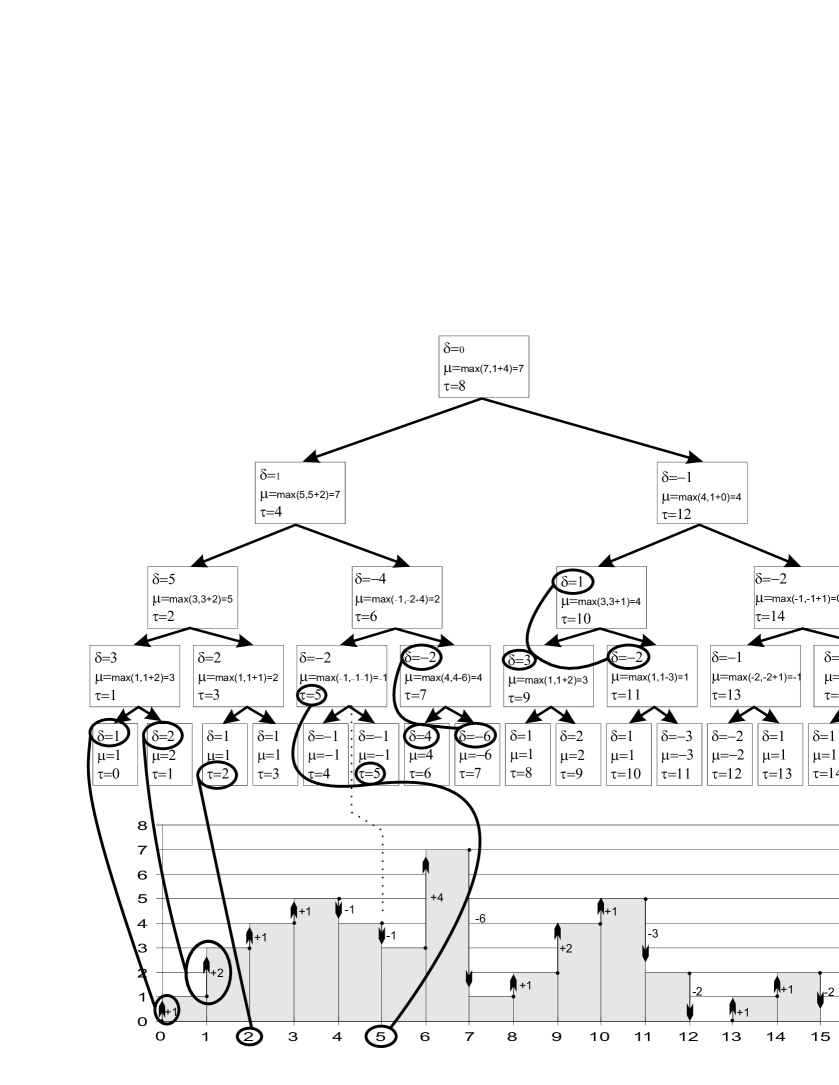
In the upper part of the figure is presented a BinSeT tree as build over the presented reservations. Additional arrows explain how particular values of , and are computed from the reservations.
In Figure 4 is shown a detail from the example.
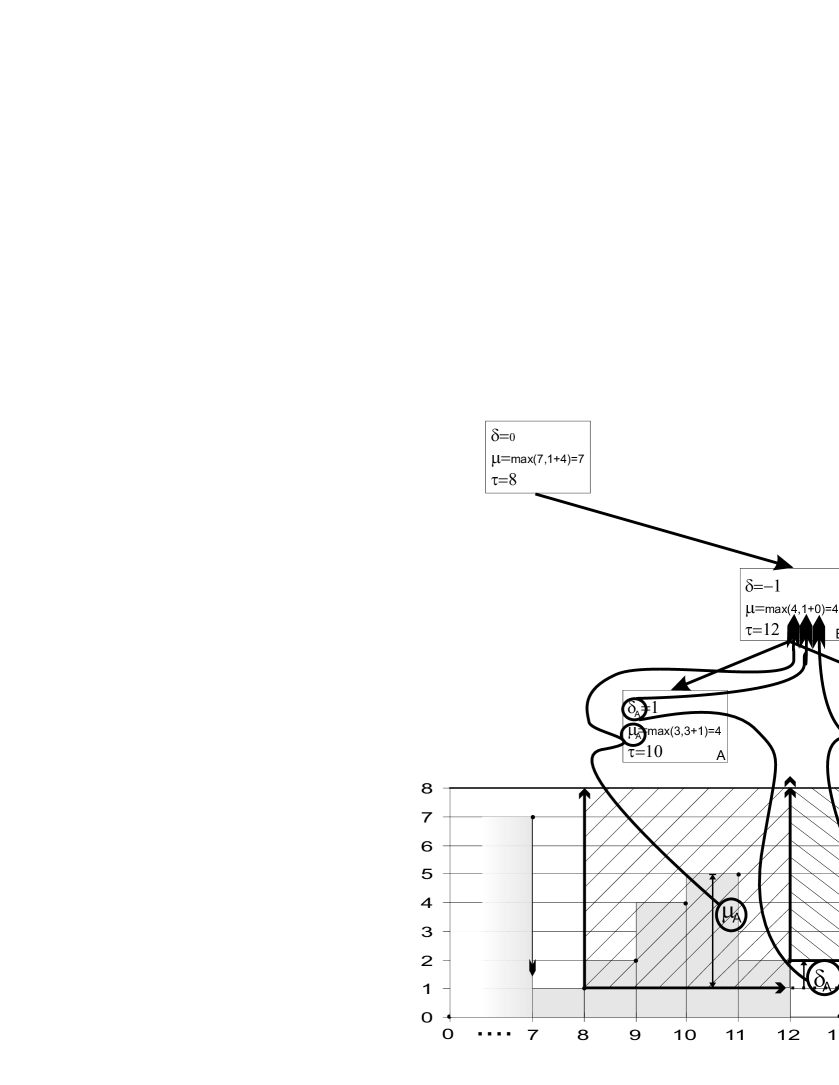
It presents “local systems” mentioned in § 3.2 for internal nodes and . The systems are presented with two different patterns: the first is expanding over slots 8 to 12 and the second one from 12 to 16. The figure also depicts and values for both nodes.