Some remarks on the survey decimation algorithm for K-satisfiability

Abstract

In this note we study the convergence of the survey decimation algorithm. An analytic formula for the reduction of the complexity during the decimation is derived. The limit of the converge of the algorithm are estimated in the random case: interesting phenomena appear near the boundary of convergence.

1 Introduction

Recently a very powerful algorithm has been proposed [1, 2] for finding the solution of the random K-satisfiability problem [3, 4, 5]. This new algorithm (see also [6, 7, 8, 9, 10]) is based on the survey-propagation equations that generalize the older approach based on the “Min-Sum” algorithm [11, 12, 15, 14] .

The aim of this note is to progress in the understanding of the deep reasons of the very good performance of this survey decimation algorithm. In the second section of this note we present a fast heuristic derivation of the survey equations. In the third section we analyze the decimation algorithm and we give an analytic formula for the decrease in the complexity during the decimation. Finally, in the fourth section we present some numerical studies of the decimation algorithm in the random case: they suggest an upper bound on the region where the algorithm may converge; we notice the appearance of new phenomena near the boundary.

2 A fast heuristic derivation of the survey equations

2.1 The random K-sat problem

In the random K-sat problem there are $N$ variable $\sigma(i)$ that may be true of false (the index $i$ will sometime called a node). An instance of the problem is given by a set of $M\equiv\alpha N$ s. For $K=3$ each clause is characterized by a set of three nodes ($i_{1}$,$i_{2}$, $i_{3}$), that belong to the interval $1-N$ and by three Boolean variables ($\beta_{1}$,$\beta_{2}$, $\beta_{3}$). In the random case the $i$ and $b$ variables are random with flat probability distribution. Each clause $c$ is true if the expression

$$E_{c}\equiv(\sigma(i^{c}_{1})\ XOR\ \beta^{c}_{1})\ OR\ (\sigma(i^{c}_{2})\ XOR\ \beta^{c}_{2})\ OR\ (\sigma(i^{c}_{3})\ XOR\ \beta^{c}_{3})$$ (1)

is true. The problem is satisfiable iff we can find a set of the variables $\sigma$ such that all the clauses are true. The entropy [14] of a satisfiable problem is the logarithm of the number of the different sets of the $\sigma$ variables that make all the clauses true.

To a given problem we can associate a graph (the factor graph [15]) where the nodes are connected to the clauses ($3\alpha$ in average) and each clause is connected to three nodes. The properties of this graph play a very important role. Some of the considerations we are going to use in the following we be valid in the random case, where when $N\to\infty$ at fixed $\alpha$ the factor graph is locally a tree.

2.2 Beliefs, warning and surveys

Generally speaking if the problem is satisfiable, very often there are many configurations of the boolean variables that satisfy it. One would like to have some description of the set of configurations that satisfy the all the clauses (in the rest of this paper we will call the configurations that satisfies all the clauses legal configurations).

In the simplest approach one introduces the strong belief or warning variable $b(i)$. They may takes tree values: true, false or unknown (in the context of colorability [8] we can introduce a new color: white [10, 6]).

In an heuristic approach one assumes that for certain values of the parameters the set of legal configurations may be decomposed into sets $C_{\gamma}$ such that each element of the set is near to the other elements of the set and is far the elements of the other sets.

For each set we define the warning corresponding to a given set according to the following rule:

• If $\sigma(i)$ is true in all the legal configurations of the set $C_{\gamma}$, $b_{\gamma}(i)$ is true.

• If $\sigma(i)$ is false in all the legal configurations of the set $C_{\gamma}$, $b_{\gamma}(i)$ is false.

• If $\sigma(i)$ is true in some legal configurations of the set $C_{\gamma}$ and it is false in some legal configurations of the same set, $b_{\gamma}(i)$ is unknown (or indifferent).

One can also introduce directional warning ($b_{\gamma}(i,c)$): they are defined to be the strong beliefs at $i$ in absence of the clause $c$ (we consider only the case where $i\in c$).

Using this definition of warning it can be argued that in the limit $N\to\infty$ for a random problem the directional warnings satisfy (or quasisatisify) the warning propagations equations (that we will write later). It is possible to argue that we can associate to any legal configuration a solution (or a quasi-solution) of the warning propagations equations, so that the legal configurations can be divided into clusters according to the solution of the warning propagation equations they correspond to [10].

A very important quantity is the number of solutions of the warning equations that correspond to some legal configuration (such a belief will be called a legal warning). This number is given by $\exp(\Sigma)$, where $\Sigma$ is called the complexity of the problem.

We would like to compute the complexity $\Sigma$ and get some information on the structure of the warnings. It argued that this can be done in the following way [1, 2]. One introduces the survey $\vec{s}(i)\equiv(s_{T}(i),s_{I}(i),s_{F}(i))$ that is a a three component vector: the probability that in the set of legal strong beliefs $b_{\gamma}(i)$ is true, indifferent and false is given by $s_{T}(i)$, $s_{I}(i)$ and $s_{F}(i)$ respectively. In a similar way we introduce the directional survey $\vec{s}(i,c)$ that is the survey at $I$ with the clause $c$ removed. Obviously a survey satisfies a normalization condition:

$$s_{T}+s_{I}+s_{F}=1\ .$$ (2)

It can be argued that for large $N$ the complexity can be approximatively written as [1, 2, 17, 18].

$$\Sigma=\sum_{i=1,N}\Sigma_{N}(i)-\sum_{c=1,M}(K(c)-1)\Sigma_{C}(c)$$ (3)

where $K(c)$ is the number of boolean variables that enters in the clause $c$. We have also defined

$$\Sigma_{C}(c)=\ln\left((1-\prod_{a=1,K(c)}(\beta_{a}^{c}\cdot\vec{s}(i_{a},c))_{F}\right)\ ,$$ (4)

where the product of a boolean variable $\beta$ with a survey $\vec{s}$ is $\vec{s}$ itself if $\beta$ is true and it is given by the vector $s_{F},s_{I},s_{T}$ if the variable $\beta$ is false ($\vec{s}_{F}$ denotes the third components of the vector $\vec{s}$).

The definition of $\Sigma_{C}(i)$ is slightly more involved. It is given by

$$\Sigma_{N}(i)=\ln\left(\left|\prod_{c\in i}\vec{u}(i,c)\right|\right)\ ,$$ (5)

where $\vec{u}(i,c)$ is a message from a clause to a node and we have defined the product of two vectors in the following way

$$\vec{v}\vec{w}=\{v_{T}\ w_{T}+v_{I}\ w_{T}+v_{T}\ w_{I}\ ,\ v_{I}\ w_{I}\ ,\ v_{F}\ w_{F}+v_{I}\ w_{F}+v_{F}\ w_{I}\}.$$ (6)

The vector $(0,1,0)$ is the identity. The norm $|\vec{v}|$ of the vector $\vec{a}$ is defined by

$$|\vec{v}|=v_{T}+v_{I}+v_{F}\ .$$ (7)

Surveys have norm 1.

We still have to define the message from a clause to node ($\vec{u}(i,c)$). It is a normalized vector $|\vec{u}(i,c)|=1$ fixed by the following condition :

$$\Sigma_{C}(c)=\ln|\vec{u}(i,c)\vec{s}(i,c)|\ ,$$ (8)

where $|\vec{u}(i,c)|$ does not depend on $\vec{s}(i,c)$. In the case where all the $b$ variables are true and an explicit computation gives

$$\vec{u}(i,c)=(f,1-f,0)\ ,\ \ \ \ \ f=\prod_{a=1,K(c),i_{a}\neq i}\vec{s}(i_{a},c))_{F}\ .$$ (9)

The quantity $\Sigma_{N}(i)$ and $\Sigma_{C}(c)$ have the meaning of the variation of the complexity when we add the node $i$ and the clause $c$ respectively.

Heuristically one suppose that the surveys satisfy the survey propagation equations that are defined to be the stationary equation of the complexity.

$${\partial\Sigma\over\partial\vec{s}(i_{a},c)}=0:$$ (10)

They can be written in an more explicit form as

$$\vec{s}(i_{a},c)={\prod_{d\in i,d\neq c}\vec{u}(i,d)\over|\prod_{d\in i,d\neq c}\vec{u}(i,d)|}\ .$$ (11)

The survey $\vec{s}(i)$ is given by the relation

$$\vec{s}(i)\propto\prod_{d\in i,}\vec{u}(i,d)\propto\vec{s}(i,c)\vec{u}(i,c)\ \ \ \forall c\in i.\ .$$ (12)

It is interesting that the warning equations have exactly the same form of the survey equations if we assume that the surveys may be only one of the following three forms: $(1,0,0)$, $(0,1,0)$ and $(0,0,1)$.  Generally speaking we will only consider in the following solutions of the surveys equations that are not of the previous form.

All this is heuristical. Independently of the derivation of the survey equations its interesting to study their properties on a random lattice. Numerical experiments and analytic computations [1, 9] suggest that in the limit $N\to\infty$ the survey equations have an unique non-trivial solutions (i.e. different from the trivial solution $s(i_{a},c)=\vec{I}$) in the interval $\alpha_{L}<\alpha<\alpha_{U}$ ($\alpha_{L}$ and $\alpha_{U}$ are are near to 3.91 and 4.36) and this unique solution may be obtained by iterations. In this interval the complexity is a decreasing function of $\alpha$ that changes sign at $\alpha^{*}\approx 4.267$.

The interval $\alpha_{L}<\alpha^{*}$ is interesting because here simple methods have difficulties in find a legal configuration. For a given problem in the interesting region we can find solutions to the survey equations. This solution carries information on the on the legal configurations so that it is natural to try to use them in an algorithm to find legal configurations.

3 Survey inspired algorithm

The basic hypothesis beyond the survey decimation algorithm is that the solution of the survey equations give reliable information on the problem. In particular we assume that:

• If the complexity is positive, there exist legal configurations and the problem is satisfiable; if the complexity is negative, there are no legal configurations and the problem is not satisfiable.

• If the survey equations have only the trivial solution ($s(i_{a},c)=\vec{I}$), the problem is easy and it can be easily solved. On the other hand if the survey equations have a non trivial solution with positive complexity, the problem has solutions but they may be difficult to be found.

Here we are taking for granted these two hypothesis. Our aim is to simplify the problem in such a way that it becomes an easy problem. This will be done using the decimation algorithm introduced in [1, 2] and described below.

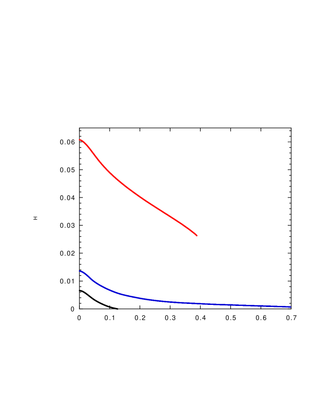
Figure 1: The complexity density $\Sigma$ as function of the fraction of decimated nodes in the region of positive complexity for a problem with $N=3\ 10^{5}$ for three values of $\alpha$ (i.e. 4.2. 4.25, 4.26 from above to below).

3.1 Decimation

If a survey ($\vec{s}_{i}$) is very near to $(1,0,0)$ (or to $(0,0,1)$) in most of the legal solutions of the warning equations (and consequently in the legal configurations) the corresponding local variables will be true (or false).

The main step in the decimation procedure consists is starting form a problem with $N$ variables and to consider a problem with $N-1$ variables where $\vec{s}(i)$ is fixed to be true (or false). We denote

$$\Delta(i)=\Sigma^{N}-\Sigma^{N-1}\ .$$ (13)

If $\Delta(i)$ is small, the second problem it is easier to solve: it has nearly the same number of solutions of the warning equations an one variable less. (We assume that the complexity can be computed by solving the survey equations.)

The decimation algorithm proceeds as follows. We reduces by one the number of variables choosing the node $i$ in the appropriate way, e.g. by choosing the variable with minimal $\Delta(i)$. We recompute the solutions of the survey equations and we reduce again the number of variables. At the end of the day two things may happen:

• We arrive to a negative complexity (in this case we are lost),

• The non trivial solution of the survey equation disappears. If this happens the reduced problem is now easy to be solved .

This program may be successfully if we have a good criterion for choosing the point $i$ and estimating $\Delta(i)$. Intuitively one would expect that if $\vec{s}(i)=(s_{T},s_{I},s_{F})$ and $s_{T}$ is large we have that

$$\Delta(i)=-\ln(1-s_{F})\ .$$ (14)

Indeed if we fix the variables $\sigma(i)$ to be true, we loose all the solutions of the warning equations such that $b(i)$ is false and therefore the total number of solutions of the warning equations should decrease by a factor $(1-s_{F})$.

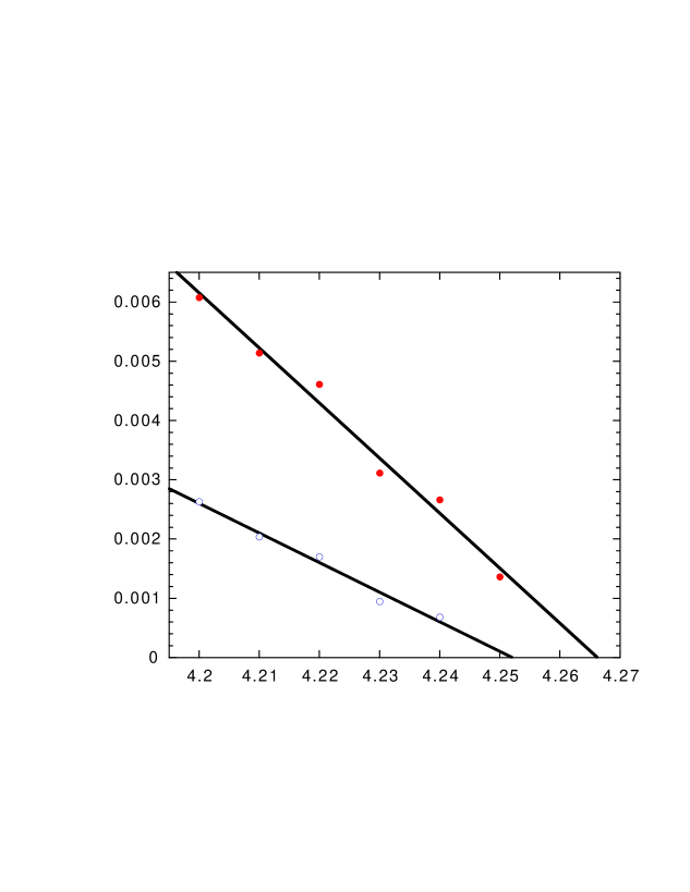
Figure 2: The initial (filled circles) and the final (empty circles) complexity density for a problem with $N=3\ 10^{5}$ as function of $\alpha$. The lines are a linear fit.

We now want to prove that this intuitive argument is correct. More precisely let us define the certitude of a survey as

$$s_{C}=\max(s_{F}+s_{I},s_{T}+s_{I})=1-\min(s_{T},s_{F})\ .$$ (15)

If $s_{C}(i,c)=1-\epsilon$, we have that

$$\Delta(i)=\ln(1-s_{C}(i))+O(\epsilon^{2})\ .$$ (16)

The crucial step consists in observing that the survey equations of the system with $N-1$ variables are the same of those of $N$ variables if we do not use the equations for $\vec{s}(i,c)$ and we set $\vec{s}(i,c)=(1,0,0)\equiv\vec{T}$. Let us call $\vec{s}^{*}$ the solutions to these new survey equations. In general $\vec{s}^{*}-\vec{s}=O(\epsilon)$. The stationary equations imply that $\Sigma^{N}(\vec{s})-\Sigma^{N}(\vec{s}^{*})=O(\epsilon^{2})$,. At the end of the computation,we find that neglecting terms of order $\epsilon^{2}$ we have:

$$\Delta(i)=\Sigma_{N}(i)-\sum_{c\in i}\ln(\vec{T}\vec{u}(i,c))\ .$$ (17)

A detailed computations shows that the r.h.s. of the previous equation is just given by $\ln(1-s_{C})$.

If we neglect the terms of order $\epsilon^{2}$, the previous argument suggests the that the best variable to be eliminated are those that have the higher certitude, or the smallest value $\min(s_{T},s_{F})$. This last criterion is similar, although different to the one used in [2], where the sites with maximum polarization, i.e. $|s_{T}-s_{F}|$. The two quantities are obviously correlated: if the polarization is near to one also the certitude is near to one.

4 The limits of the algorithm.

Here in order to illustrate how the algorithm works we report for completeness the results of a few numerical experiments we have done on large samples (from $N=10^{4}$ to $N=3\ 10^{5}$ near $\alpha^{*}$ where (for fastening the algorithm) a fraction $f=10^{-4}$ of the total variables has been decimated simultaneously. In fig. (1) for one sample with $N=3\ 10^{5}$ we plot the complexity as function of the number of iterations for three different values of $\alpha$ where we have blocked the surveys with maximal polarization. We see that for the low value of $\alpha$ the method does work, the complexity jumps to zero coming from a positive value, while for the high value of $\alpha$ the complexity becomes negative. A very similar is obtained is done in the case where we select the surveys using the maximum value of the certitude.

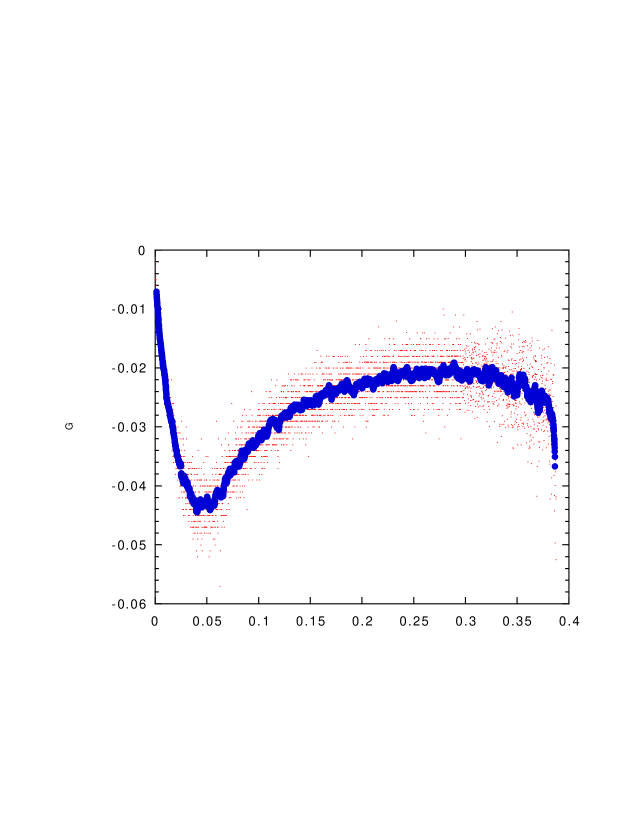
Figure 3: The quantities $1-s_{F}(i)$ (continuos curve) and the quantity $\Delta(i)$, averaged on a window of ten decimations (scattered points) of as function of the fraction of decimated nodes for one problem with $N=3\ 10^{5}$ and $\alpha=4.2$. The variable $i$ is the decimated node.

In fig 2 we plot the complexity density $\Sigma_{M}/M$ ($M$ is the number of undecimated nodes) at the starting point and at the final point of the decimation procedure. We see that the initial complexity density extrapolates to zero at $\alpha\approx 4.267$ (in perfect agreement with the analytic estimates [1, 2].) while the final complexity becomes negative at $\alpha_{A}\approx 4.252$. Similar results are obtained for smaller values of $N$.

The conclusion is that in the present form the survey decimation algorithm may work in the infinite $N$ limit for $\alpha<\alpha_{A}\approx 4.253<\alpha_{c}$. The numerical experiments seem also to indicate that near $\alpha_{A}$ the complexity becomes negative near $f=1$. The reasons for this remarkable phenomenon will not be discussed here.

Very similar results are obtained if we use the certitude $s_{C}(i)$ to select the spins: there are very minor differences which need a very careful analysis to be evidenziated at least if we are not to near to $\alpha_{A}$, that may slightly depends on the method used. En passant we have also verified that the quantity $s_{C}(i)$ is strongly correlated with $\Delta(i)$ and the high order terms in $\epsilon$ are nor very important. In fig. (3) we see for $N=3\ 10^{5}$ and $\alpha=4.2$ these two quantities as function of $f$. It is remarkable that in the average these two quantities coincide, i.e. if we smooth $\Delta(i)$ on a sufficiently large window it becomes very near to $1-s_{F}(i)$

The behaviour of the polarization (i.e. $|s_{T}-s_{F}|$) of the chosen variable as function of the fraction $f$ of removed variables is very similar to that of the certitude (the two quantities are strongly correlated) and it is shown in fig. (4).

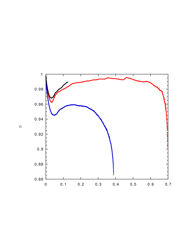
Figure 4: The polarization $|s_{T}-s_{F}|$ of as function of the fraction of decimated nodes for one problem with $N=3\ 10^{5}$ and $\alpha=4.2,\ 4.25,\ 4.26$ from below to above.

The behaviour of both quantities is remarkable. The behavior for small $f$ (e.g. $f<.02$) can be easily understood and it can be obtained from the distribution of the surveys of the undecimated problem. The increase of the polarization of the chosen spin after the minimum around $f<\approx 05$ is an effect of computing the solution of the surveys equation in the decimated problem. It is a very interesting phenomenon and it is at the root of the good performances of the survey decimation algorithm.

The numerical experiments seem also to indicate that near $\alpha_{A}$ the value of $f$ where the complexity becomes negative goes to one, al least with the algorithm where the decimated clause has the maximal certitude. In fig. (5) we see the complexity as function of $f$ for a sample with $N=3\ 10^{5}$ and $\alpha=4.2525$. Here the complexity jumps to zero at $f=.993$. However one should do a more careful and accurate finite size analysis data to see how this effect depends on the algorithm and on the sample.

Let us just sketch a simple intuitive argument for explaining this behaviour of the system. Let us assume that:

• The complexity can jump to zero when the non-trivial solution of the survey disappear only if the value of the complexity is near to zero or negative.

• The probability for the decimation process to be stopped by the presence of a zero in the denominator of eq. 11 is is small for small $\Sigma$ and it has a natural prefactor that diverges when $f$ goes to one.

• At fixed $f$ the complexity is a decreasing function of $\alpha$: $\partial\Sigma(f,\alpha)/\partial\alpha<0$.

If the maximum value of $f$ would be less than one at $\alpha_{A}$, we would find a contradiction in the behaviour at $\alpha$ slightly greater that $\alpha_{A}$: the survey decimation process would end with a jump from a negative complexity and this is prohibited. The contradiction would not be present if the maximum value of $f$ is 1, because the stopping probability diverges here.

In order to explain the performances of the algorithm it would important to find a more direct argument that the maximum value of $f$ is 1 at $\alpha_{c}$.

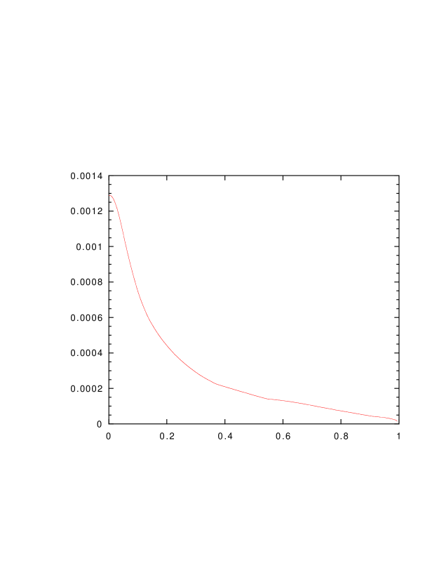
Figure 5: The complexity as function of the fraction $f$ fraction of decimated nodes for one problem with $N=3\ 10^{5}$ and $\alpha=4.2525$ The complexity jumps to zero at $f=.993$ where the number of undecimated clauses is about 2000.

5 Conclusion

The main result of this paper is the identification of the quantity (i.e. the certitude $1-\min(s_{T},s_{F})$) that controls the complexity reduction during the decimation and the identification of the threshold value of $\alpha_{A}$ where the decimation algorithms must stop to work. Numerical simulations indicate that interesting phenomena happens near $\alpha_{A}$, however a more careful investigation is needed in order to properly quantify them. An analytic understanding of these phenomena is lacking at the present moment: it would be very important to obtain it because it would a key step in understanding the reasons for the good performances of the survey decimation algorithm.

References

- [1] M. Mézard, G. Parisi and R. Zecchina, Science 297, 812 (2002).
- [2] M. Mézard and R. Zecchina The random K-satisfiability problem: from an analytic solution to an efficient algorithm cond-mat 0207194.
- [3] S. Kirkpatrick, B. Selman, Critical Behaviour in the satisfiability of random Boolean expressions, Science 264, 1297 (1994)
- [4] Biroli, G., Monasson, R. and Weigt, M. A Variational description of the ground state structure in random satisfiability problems, Euro. Phys. J. B 14 551 (2000),
- [5] Dubois O. Monasson R., Selman B. and Zecchina R. (Eds.), Phase Transitions in Combinatorial Problems, Theoret. Comp. Sci. 265, (2001);
- [6] A. Braustein, M. Mezard, M. Weigt, R. Zecchina: cond-mat/0212451 Constraint Satisfaction by Survey Propagation.
- [7] A. Braunstein, M. Mezard, R. Zecchina; cs.CC/0212002 Survey propagation: an algorithm for satisfiability.
- [8] R. Mulet, A. Pagnani, M. Weigt, R. Zecchina: cond-mat/0208460 Coloring random graphs.
- [9] G. Parisi: CC/0212047 On local equilibrium equations for clustering states
- [10] G. Parisi cs.CC/0212009 On the survey-propagation equations for the random K-satisfiability problem
- [11] J.S. Yedidia, W.T. Freeman and Y. Weiss, Generalized Belief Propagation, in Advances in Neural Information Processing Systems 13 eds. T.K. Leen, T.G. Dietterich, and V. Tresp, MIT Press 2001, pp. 689-695.
- [12] Mézard, M., Parisi, G. and Virasoro, M.A. Spin Glass Theory and Beyond, World Scientific, Singapore, 1987.
- [13] D.J. Thouless, P.A. Anderson and R. G. Palmer, Solution of a ‘solvable’ model, Phil. Mag. 35, 593 (1977).
- [14] Monasson, R. and Zecchina, R. Entropy of the K-satisfiability problem, Phys. Rev. Lett. 76 3881–3885(1996).
- [15] F.R. Kschischang, B.J. Frey, H.-A. Loeliger, Factor Graphs and the Sum-Product Algorithm, IEEE Trans. Infor. Theory 47, 498 (2002).
- [16] O. Dubois, Y. Boufkhad, J. Mandler, Typical random 3-SAT formulae and the satisfiability threshold, in Proc. 11th ACM-SIAM Symp. on Discrete Algorithms, 124 (San Francisco, CA, 2000).
- [17] M. Mézard and G. Parisi, Eur.Phys. J. B 20 (2001) 217.
- [18] M. Mézard and G. Parisi, ‘The cavity method at zero temperature’, cond-mat/0207121 (2002).