Temporal plannability by variance of the episode length

Abstract.

Optimization of decision problems in stochastic environments is usually concerned with maximizing the probability of achieving the goal and minimizing the expected episode length. For interacting agents in time-critical applications, learning of the possibility of scheduling of subtasks (events) or the full task is an additional relevant issue. Besides, there exist highly stochastic problems where the actual trajectories show great variety from episode to episode, but completing the task takes almost the same amount of time. The identification of sub-problems of this nature may promote e.g., planning, scheduling and segmenting Markov decision processes. In this work, formulae for the average duration as well as the standard deviation of the duration of events are derived. The emerging Bellman-type equation is a simple extension of Sobel’s work (1982). Methods of dynamic programming as well as methods of reinforcement learning can be applied for our extension. Computer demonstration on a toy problem serve to highlight the principle.

1. Motivation

There is an increasing interest in planning in stochastic environments, also called decision-theoretic planning. Since planning is admired as a mainstay of artificial intelligence, attempts were made to extend classical AI planning methods to handle uncertainty. On the other hand, operations research has made important advances recently in solving decision making problems [23]. One of the earliest works, which tried to unify the two complementary approaches appeared in the seventies [6]. Recently Markov decision processes are proposed as a unifying framework for decision-theoretic planning [2, 5]. The success of the closely related reinforcement learning (RL) techniques have encouraged work in planning using Markov decision processes.

For planning one needs goals. Classical AI planning usually determines the goal as a subset of the state space. This definition is extended by Markov decision processes, where an immediate cost (or reward) function is defined and the ‘goal’ of the decision maker is not to reach a set of states, but to minimize the discounted long-term cumulated cost. In RL, planning is equal to finding ‘good’ policies, i.e. state-dependent action selection strategies for which the cumulated cost is minimal [15]. In Markov decision processes, one speaks of episodic tasks, when well-defined terminal (goal) states exist and the episode as well as the accumulation of costs stops in finite time — after reaching one of the terminal states. In episodic tasks, planning is often formalized as the task of finding plans for which the probability of achieving the goal states is maximal and/or the expected episode length is minimal.

The suggested plans may have many evaluation criteria, such as the average cost accumulated during execution, the probability of a successful execution, or the expected episode length. We will focus here on a rarely emphasized feature of plans, namely the reliability of the plan execution time, which is an important issue in time-sensitive systems. For example, imagine a cooperating multi-agent system, where the agents can interact only if they are close in space (e.g. the agents are the trucks of a transport company). It is impossible to create a global long-term plan if the arrival time of specific agents (trucks) show a great variety. Being accurate in the time of arrival may be much more important than having somewhat faster deliveries on the average. Another example is that ‘the postman may bring a letter at 8 o’clock’. It might be important to check the mailbox, although the probability of receiving an answer is low. Missing an appointment may cause long-term effects in the whole system like a small snowball can grow into an avalanche. This is a relevant issue in every system with strongly nonlinear responses, which is the common cause in the engineering practice. In most real-life problems, for long-term planning nearly-deterministic (i.e., reliable) sub-components (sub-tasks) are necessary. A number of possible applications are mentioned at the end of the paper.

How to measure reliability? The simplest assumption is that the larger the variance of the duration of a sub-task, the less one can rely on that component when making a plan. In the next section we propose a simple algorithm for calculating the time variance of episodes.

2. Calculating the duration and the variance of the duration of episodes

2.1. Assumptions and definitions

Consider an episodic MDP with a finite state space $S$ and a finite action space $A$. The agent starts from some state $x_{0}$, and makes steps according to policy $\pi:S\times A\to[0,1]$ until it reaches a state in the terminal set $Z\subset S$. Let $Z_{0}\subset Z$ be the goal set. We may assume that from any terminal state $z\in Z$, the agent is transferred to a hyper-terminal state $\omega$, i.e. $P(z,a,\omega)$=1 for all $z\in Z,a\in A$. This assumption does not modify the time of reaching $Z$ for the first time, but it enables us to simplify our formalism, because every state in $Z$ is visited at most once.

Denote by $p^{\pi}(x,y)$ the probability that from state $x$ the agent arrives to state $y$ while following policy $\pi$, i.e.

(1) $$p^{\pi}(x,y)=\sum_{a\in A}\pi(x,a)P(x,a,y).$$

The visited states in a start-goal episode are noted by $\left\{b_{0},\ldots,b_{K}\right\}$ assuming the episode takes $K$ steps (note that $K$ is also a random variable). If an $x\rightarrow y$ transition takes $\tau_{xy}\in\mathcal{N}_{0}$ time, then the completion time of an episode can be calculated as $T=\sum_{i=0}^{K-1}\tau_{b_{i}b_{i+1}}$ where $T\in\mathcal{N}_{0}$. Naturally, if every transition takes 1 unit of time then $K\equiv T$.

We would like to find the answer to the following three questions:

1. What is the probability that the agent ends up in a goal state, i.e. in $Z_{0}$?

2. What is the average time needed for reaching a goal state?

3. What is its variance?

2.2. The probability of success

An episode may be either successful (the agent ends up in $Z_{0}$) or unsuccessful (the agent ends up in $Z\backslash Z_{0}$). Denote by $s(x)$ the probability that starting from $x$, the agent will be successful, i.e. $s(x)=\Pr(b_{K}\in Z_{0}|b_{0}=x)$. Clearly,

(2) $$s(x)=\begin{cases}1&\text{if $x\in Z_{0}$},\\ 0&\text{if $x\in Z\backslash Z_{0}$},\\ \sum_{y\in S}p^{\pi}(x,y)s(y)&\text{if $x\in S\backslash Z$}.\end{cases}$$

2.3. The probability of success in exactly T time

Let $q(T|x)$ denote the probability of reaching $Z_{0}$ exactly at time $T$, assuming the agent started from state $x$ at time $0$. That is, $q(T|x)=\Pr(T,b_{K}\in Z_{0}|b_{0}=x)$ for every $T\geq 0$. Then,

$$q(0|x)=\begin{cases}1&\text{if $x\in Z_{0}$},\\ 0&\text{if $x\in S\backslash Z_{0}$},\end{cases}$$

and the following simple recursion holds:

$$q(T|x)=\begin{cases}\sum_{y\in S}p^{\pi}(x,y)q(T-\tau_{xy}|y)&\text{if $x\in S\backslash Z$ }\\ 0&\text{if $x\in Z$}\end{cases}$$

for $T\geq 1$ and $q(T|x)=0$ for every $T<0$.

For the sake of simplicity, we assume that from any non-terminal state the agent reaches a terminal state in finite time with probability one, i.e.

$$\{\Pr(b_{K}\notin Z_{0}|b_{0}=x),q(0|x),q(1|x),q(2|x),\ldots\}$$

is a probability distribution. It is easy to see that $\sum_{T=0}^{\infty}q(T|x)=s(x)$.

2.4. The average episode length

Making use of the above recursion, similar recursion can be derived for the expected number of time steps needed to reach a goal state from $x$ (denoted by $A(x)$):

$$A(x) = \mathbf{E}(T|b_{K}\in Z_{0},b_{0}=x)=\sum_{T=0}^{\infty}T\cdot\Pr(T|b_{K}\in Z_{0},b_{0}=x)=$$

$$= \sum_{T=0}^{\infty}T\cdot\frac{\Pr(T,b_{K}\in Z_{0}|b_{0}=x)}{\Pr(b_{K}\in Z_{0}|b_{0}=x)}=\frac{1}{s(x)}\sum_{T=0}^{\infty}T\cdot q(T|x).$$

In particular, if $x\in Z$, then $A(x)=0$. For $x\in S\backslash Z$, $A(x)$ can be expressed as

(3) $$A(x) = \frac{1}{s(x)}\sum_{T=0}^{\infty}T\cdot q(T|x)=$$

$$= \frac{1}{s(x)}\sum_{T=0}^{\infty}T\sum_{y\in S}p^{\pi}(x,y)q(T-\tau_{xy}|y)=$$

$$= \frac{1}{s(x)}\sum_{y\in S}p^{\pi}(x,y)\sum_{T=0}^{\infty}\bigl{[}(T-\tau_{xy})\cdot q(T-\tau_{xy}|y)+\tau_{xy}q(T-\tau_{xy}|y)\bigr{]}=$$

$$= \frac{1}{s(x)}\sum_{y\in S}p^{\pi}(x,y)\left(\sum_{T=0}^{\infty}T\cdot q(T|y)+\tau_{xy}\sum_{T=0}^{\infty}q(T|y)\right)=$$

$$= \frac{1}{s(x)}\sum_{y\in S}p^{\pi}(x,y)s(y)\left[A(y)+\tau_{xy}\right].$$

2.5. The variance of episode length

The second moment $B(x)$ of the episode length for each $x\in S$ can be derived in a similar manner:

$$B(x)=\mathbf{E}(T^{2}|b_{K}\in Z_{0},b_{0}=x)=\frac{1}{s(x)}\sum_{T=0}^{\infty}T^{2}\cdot q(T|x).$$

If $x$ is a terminal state, then $B(x)=0$. Otherwise,

(4) $$B(x) = \frac{1}{s(x)}\sum_{T=0}^{\infty}T^{2}\cdot q(T|x)=\frac{1}{s(x)}\sum_{T=0}^{\infty}T^{2}\sum_{y\in S}p^{\pi}(x,y)q(T-\tau_{xy}|y)=$$

$$= \frac{1}{s(x)}\sum_{y\in S}p^{\pi}(x,y)\cdot\sum_{T=0}^{\infty}\bigl{[}(T-\tau_{xy})^{2}\cdot q(T-\tau_{xy}|y)+$$

$$+ 2\cdot\tau_{xy}\cdot T\cdot q(T-\tau_{xy}|y)-\tau_{xy}^{2}q(T-\tau_{xy}|y)\bigr{]}=$$

$$= \frac{1}{s(x)}\sum_{y\in S}p^{\pi}(x,y)\cdot\sum_{T=0}^{\infty}\bigl{[}(T-\tau_{xy})^{2}\cdot q(T-\tau_{xy}|y)+$$

$$+ 2\cdot\tau_{xy}\left[(T-\tau_{xy})\cdot q(T-\tau_{xy}|y)+\tau_{xy}\cdot q(T-\tau_{xy}|y)\right]-$$

$$- \tau_{xy}^{2}q(T-\tau_{xy}|y)\bigr{]}=\frac{1}{s(x)}\sum_{y\in S}p^{\pi}(x,y)\cdot$$

$$\cdot \left(\sum_{T=0}^{\infty}T^{2}\cdot q(T|y)+2\cdot\tau_{xy}\sum_{T=0}^{\infty}T\cdot q(T|y)+\tau_{xy}^{2}\sum_{T=0}^{\infty}q(T|y)\right)=$$

$$= \frac{1}{s(x)}\sum_{y\in S}p^{\pi}(x,y)s(y)\left[B(y)+2\cdot\tau_{xy}\cdot A(y)+\tau_{xy}^{2}\right].$$

By the well known formula, the variance is

(5) $$D(x)=\sqrt{B(x)-A(x)^{2}}.$$

These recursive equations form the base of an algorithm: first, iterate the $s(x)$ quantity according to Eq. (2), until equilibrum is reached, second, iterate $A(x)$ using Eq. (3) with the previously calculated $s(x)$, third, iterate $B(x)$ with Eq. (4) using $s(x)$ and $A(x)$. The resulting method gives (i) the probability of success, (ii) the time an episode takes on average, and (iii) the variance of the episode time from all possible starting states for a prescribed terminal state set.

3. Demonstration

We generated a simple toy problem to demonstrate the utility of the algorithm. Imagine a river, which flows rapidly from west to east. There is a port on the left bank of the river. There is also a ship on the river, initially positioned somewhere on the river. The ship has to reach the port, otherwise it enters a terrible and huge waterfall, situated at the east end of the river. The water has very strong vortices and currents, therefore it is almost impossible to control the movement of the ship. Our model assumes that in the next time step the currents will almost surely drive the ship towards the waterfall, but we don’t know exactly in which direction. A small chance exists that the vortices drive the ship backwards, too. Of course, at a given instant, and if not at the east end of the river, the ship can’t be very far from its previous position. Details of this toy problem are depicted in Fig. 1. This example has a few situations, which will occur with high probabilities: every transition (except for the ones near the banks) has low probability to be happened. Direct planning of particular trajectories is almost meaningless. But, as it can be seen on Figs. 3 and 4, temporal planning, in the sense defined in Section 2, is still meaningful. Figures 2, 3 and 4 plot the quantities $s(x)$, $A(x)$ and $C(x)$ respectively, after reaching equilibrium (we performed 100 iterations). The figures show that there is a very low chance to reach the port when the ship starts behind it, as expected. However, because we calculate the time needed for successful episodes, the average episode times needed are almost the same as when the ship starts in the leftmost positions, but the reliability of these times – measured by the variance (Fig. 4) – are higher in the first case. If the harbor master knows the ship’s starting position, than he knows when to look for the ship on the horizon according to Fig. 3, and he can decide from Fig. 4 how long should he wait until he can almost surely guess that the ship is lost.

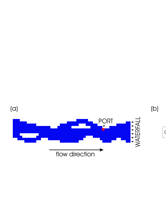
Figure 1. Description of the toy problem.
Subfigure (a) shows the ‘river’ flowing from the left to the right. The river is constructed on a 50 by 10 square grid. The ‘port’ is marked with a red square. The river empties into a waterfall on the right side. If the ship reaches any states of the last column, the trial has an unsuccessful end. Subfigure (b) shows the predefined state transitions. If not obstructed by the river’s bank, there is an equal probability (0.3) of transferring from the current state (noted by C.S.) into one of the three neighboring states in the next right column. The diagonal steps take 2 time units, while the forward step takes 1 time unit. Simultaneously, there is also a low probability (0.1) of moving backwards to the left column, which move takes 5 time units. The banks of the river and the islands limit the number of available transitions. In this cases, the probability of the unavailable transition(s) is equally distributed between the remaining ones.

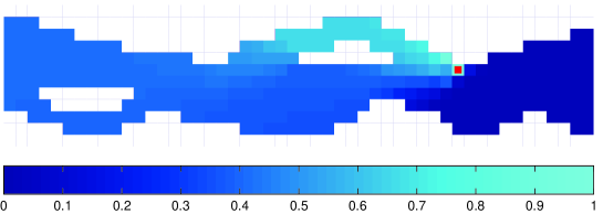
Figure 2. Probability of a successful episode.
The figure plots the probability of successful arrivals from any given state ($s(x)$) (computed by the recursive formula (2). The graded blue color of a point of the river provides the probability of arriving to the port. Color coding is provided at the bottom of the figure. The dark colors on the right hand side of the port indicate that chances of successful arrivals from that part of the river are low.

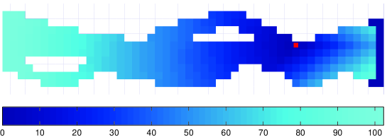
Figure 3. Average episode lengths.
Average durations ($A(x)$) of successful episodes are indicated by graded blue color for every state ($x$).

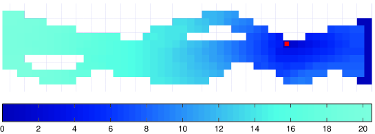
Figure 4. Variance of episode length.
The variance of the duration of successful episodes ($C(x)$) are indicated by graded blue color for every state $(x)$.

4. Discussion

Examining the probabilistic properties of the cumulated cost beyond its average value is not new in the literature. The attempts concentrated mainly on penalizing the variance of the accumulated cost [7, 9, 10, 25, 26, 3]. Algorithms for calculating the variance directly have also been published. Kemeny and Snell ([11]) developed a formula for the second moment of first-passage times in Markov chains. Formulae are derived in [18] for the second moment of the accumulated total reward of Markov chains with rewards. In [21] Sobel presented a general method for calculating the arbitrary moments of the cumulated discounted cost. This method is similar to ours. The algorithm introduced here emphasizes the possibility of using the average duration of the episode, or higher moments of the duration of an episode as costs to transfer the problem of plannability to the domain of reinforcement learning, as it will be discussed shortly. By introducing the probability of success, a novel property of the formulae is that they can be used to compute the appropriate properties for successful or unsuccessful episodes.

4.1. Reinforcement Learning Methods

The algorithm does not employ the immediate costs (rewards) defined by the original MDP. Nevertheless, the algorithm is closely related to such cost-based approaches: If the transition time is viewed as cost, then calculating the average time of the execution of the episode can be seen as calculating the average sum of the (time-)costs in the non-discounted case. In this sense, the quantities $\tau_{xy}$ determine the corresponding cost function. Indeed, we can recognize Eq. 4 as the well-known Bellman-equality [1] for the case of non-discounted costs.

Therefore, similarly to the standard reinforcement learning problem, we do not need to solve the DP equations directly, but we may update the $s$, $A$ and $B$ values in different ways explored by theoretical works in the field of RL (for a historical review, see, e.g., [24] and references therein). Asynchronous and Monte Carlo methods, as well as sampling methods analogous to Q-learning or SARSA can be of use here. The advantage of RL methods as compared to DP methods can be seen in problems that are too large for direct computations. Moreover, RL methods can be used by direct interaction with the system (called on-line learning). This solution is the only option when no model is available. On the other hand, if a DP model is available and sampling methods with the real system are cumbersome, then DP has the advantage of being an off-line method, not limited by constraints on interactions with a real system.

Another advantage of formulating temporal planning within the framework of RL is that costs on time (i.e., planning) and real costs of the episode can be unified into a single cost function. Moreover, the multi-criteria paradigm [17, 8] can be applied to consider multiple cost functions in parallel. In particular, cost functions with mean-variance tradeoffs [7, 10, 25, 26, 3] may penalize solutions with high variance. One has the option of solving the MDP for the original cost function and also for the time as the ‘cost’ and then combine the two aspects.

4.2. Planning as a Segmentation Tool

As it has been mentioned before, in our terminology planning is an off-line method, which serves to minimize the frequency of on-line decision making. Planning can be the tool to segment decision making problems into subproblems.

In practice, the major problem of decision-theoretic planning is the intractably large space state. Handling complex, real-life situations is impossible without grouping states into larger sets (possibly structured in hierarchical fashion), thus allowing for crude discretization, partial observation and assigning subgoals for complex tasks. In most real-life problems, the environment is only partially observable, therefore we need to solve partially observable Markov decision processes instead of classical MDPs. Partial observability may come from the limited perceptual capabilities of the agent: the agent may possess insufficient resources to observe all variables of its environment, the agent may be localized not having information about remote objects in space, the agent may be slow to observe all temporal changes happening in the environment. If the optimization problem is partially observable, then solving this problem is intractable in general [14]. Every available tool should be used to ease the learning problem. The most promising methods are those, which are only partly limited by the number of interactions with the real system, that is, the on-line methods extended by off-line methods. Off-line computations are preferred when they are relatively inexpensive. These methods may be able to segment the current problem into subproblems. One of the candidates for finding a suitable segmentation is the temporal reliability measured by the variance of the duration of the episode or a part of the episode. One can use the variance calculated by Eq. (5) to measure which states are reliable subgoals. Then, variance of the duration of the episode serves as auxiliary information for distinguishing states which can be later assigned as subgoals. The advantages of subgoals and concept formation using subgoals have been in the focus of recent research interest (see, e.g., [19, 20, 27, 22, 16] and references therein).

These concepts may gain applications in a variety of areas: basically everywhere, where RL and DP need to be extended by scheduling. A few representative examples are as follows: job-shop scheduling [28], elevator optimization [4], robotic soccer [12] or context focused Internet crawling making use of RL [13].

5. Acknowledgements

This work was supported by the Hungarian National Science Foundation (Grant OTKA 32487) and by EOARD (Grant F61775-00-WE065). Any opinions, findings and conclusions or recommendations expressed in this material are those of the authors and do not necessarily reflect the views of the European Office of Aerospace Research and Development, Air Force Office of Scientific Research, Air Force Research Laboratory.

References

- [1] R. Bellman, Dynamic programming, Princeton University Press, Princeton, New Jersey, 1957.
- [2] C. Boutilier, T. Dean, and S. Hanks, Decision-theoretic planning: Structural assumptions and computational leverage, Journal of Artificial Intelligence Research 11 (1999), 1–99.
- [3] E. J. Collins, Finite-horizon variance penalised markov decision processes, OR Spektrum 19 (1997), 35–39.
- [4] R. H. Crites and A. G. Barto, Improving elevator performance using reinforcement learning, Advances in Neural Information Processing Systems (San Mateo, CA) (M. C. Mozer D. S. Touretzky and M. E. Hasselmo, eds.), vol. 8, Morgan and Kaufmann, 1996, pp. 1017–1023.
- [5] T. Dean, L. Kaelbling, J. Kirman, and A. Nicholson, Planning under time constraints in stochastic domains, Artificial Intelligence 76 (1995), no. 1-2, 35–74.
- [6] J. A. Feldman and R. F. Sproull, Decision theory and artificial intelligence II: The hungry monkey, Cognitive Science 1 (1977), 158–192.
- [7] J. A. Filar, L. C. M. Kallenberg, and H. M. Lee, Variance-penalised markov decision processes, Math Oper. Res. 14 (1989), 147–161.
- [8] Z. Gábor, Zs. Kalmár, and Cs. Szepesvári, Multi-criteria reinforcement learning, Proceedings of the Fifteenth International Conference on Machine Learning, 1998.
- [9] J.J. Greffenstette, C.L. Ramsey, and A.C. Schultz, Learning sequential decision rules using simulation models and competition, Machine Learning 5 (1990), 355–381.
- [10] Y. Huang and L. C. M. Kallenberg, On finding optimal policies for markov decision chains: a unifying framework for mean-variance-tradeoffs, Math Oper. Res. 19 (1994), 434–448.
- [11] J. G. Kemeny and J. L. Snell, Finite markov chains, Van Nostrand, New York, 1960.
- [12] H. Kitano, M. Asada, Y. Kuniyoshi, I. Noda, and E. Osawa, RoboCup: The robot world cup initiative, Proceedings of the First International Conference on Autonomous Agents (Agents’97) (New York) (W. Lewis Johnson and Barbara Hayes-Roth, eds.), ACM Press, 5–8, 1997, pp. 340–347.
- [13] I. Kókai and A. Lőrincz, Fast adapting value estimation based hybrid architecture for searching the world-wide web, Applied Soft Computing, (in press).
- [14] M. L. Littman, Algorithms for sequential decision making, Ph.D. thesis, Department of Computer Science, Brown University, February 1996.
- [15] M. L. Littman, J. Goldsmith, and M. Mundhenk, The computational complexity of probabilistic planning, Journal of Artificial Intelligence Research 9 (1998), 1–38.
- [16] A. McGovern, Autonomous discovery of temporal abstractions from interaction with an environment, Phd thesis, University of Massachusetts, Amherts, MA, 2002.
- [17] L. G. Mitten, Composition principles for synthesis of optimum multi-stage processes, Operations Research 12 (1964), 610–619.
- [18] L. K. Platzman, Mimeographed lecture notes for ioe 315., Dept. of Industrial and Operations Engineering, University of Michigan, Ann Arbor, 1978.
- [19] M. Ring, Incremental development of complex behaviors through automatic construction of sensory-motor hierarchies, Proceedings of the Eighth International Conference on Machine Learning (San Mateo, CA), Morgan Kaufmann, 1991.
- [20] J. Schmidhuber, Artificial neural networks, eds.: T. kohonen, k. mäkisara, o. simula, and j. kangas, ch. Learning to generate sub-goals for action sequences, pp. 967–972, Elsevier Science Publishers, 1991.
- [21] M. J. Sobel, The variance of discounted Markov decision processes, Journal of Applied Probability 19 (1982), 794–802.
- [22] R. Sun and C. Sessions, Self-segmentation of sequences: automatic formation of hierarchies of sequential behaviors, IEEE Transactions on Systems, Man, and Cybernetics: Part B Cybernetics 30 (2000), 403–418.
- [23] R. Sutton, Dyna, an integrated architecture for learning, planning, and reacting, SIGART Bulletin 2 (1991), 160–163.
- [24] R. Sutton and A. G. Barto, Reinforcement learning: An introduction, MIT Press, Cambridge, 1998.
- [25] D. J. White, Computational approaches to variance penalised markov decision processes, OR Spektrum 14 (1992), 79–83.
- [26] by same author, A mathematical programming approach to a problem in variance penalised markov decision processes, OR Spektrum 15 (1994), 225–230.
- [27] M. Wiering and J. Schmidhuber, HQ-learning: Discovering markovian subgoals for non-markovian reinforcement learning, Technical Report IDSIA-95-96, 1996.
- [28] W. Zhang and T. G. Dietterich, A reinforcement learning approach to job-shop scheduling, Proceedings of the International Joint Conference on Artificial Intellience, 1995.