Confluent Drawings:
Visualizing Non-planar Diagrams in a Planar Way

Abstract

In this paper, we introduce a new approach for drawing diagrams that have applications in software visualization. Our approach is to use a technique we call confluent drawing for visualizing non-planar diagrams in a planar way. This approach allows us to draw, in a crossing-free manner, graphs—such as software interaction diagrams—that would normally have many crossings. The main idea of this approach is quite simple: we allow groups of edges to be merged together and drawn as “tracks” (similar to train tracks). Producing such confluent diagrams automatically from a graph with many crossings is quite challenging, however, so we offer two heuristic algorithms to test if a non-planar graph can be drawn efficiently in a confluent way. In addition, we identify several large classes of graphs that can be completely categorized as being either confluently drawable or confluently non-drawable.

1 Introduction

Software visualization is often done through the use of diagrams constructed so that important components, entities, agents, or objects are drawn as simple shapes, such as circles or boxes, and relationships are drawn as individual curves connecting pairs of these shapes. That is, such visualizations are done by drawing graphs in a standard way, so as to assign vertices to points (or simple shapes) and to assign edges to simple paths connecting pairs of vertices (e.g., see [15, 17, 28]). Examples of such software visualizations include data flow diagrams [2], object-oriented class hierarchies [5, 37], object-interaction diagrams [4], method-call graphs [22, 24, 41], as well as the classic application of flowcharts [29] (see also [1, 34, 36, 39]). Moreover, these examples include both directed and undirected diagrams.

In addition, it is quite common for software visualizations to be constructed automatically rather than being hand-crafted. Thus, there is a need for efficient algorithms that produce aesthetically-pleasing diagrams for software visualizations.

1.1 Related Prior Work

There are several aesthetic criteria that have been explored algorithmically in the area of graph drawing (e.g., see [15, 17, 28]). Examples of aesthetic goals designed to facilitate readability include minimizing edge crossings, minimizing a drawing’s area, and achieving good separation of vertices, edges, and angles. Of all of these criteria, however, the arguably most important is to minimize edge crossings, since crossing edges tend to confuse the eye when one is viewing adjacency relationships. Indeed, an experimental analysis by Purchase [35] suggests that edge-crossing minimization [25, 26, 30] is the most important aesthetic criteria for visualizing graphs. Ideally, we would like drawings that have no edge crossings at all.

Graphs that can be drawn in the standard way in the plane without edge crossings are called planar graphs [32], and there are a number of existing efficient algorithms for producing crossing-free drawings of planar graphs (e.g., see [8, 9, 10, 6, 11, 16, 13, 21, 23, 27, 38, 40]).

Unfortunately, most graphs are not planar; hence, most graphs cannot be drawn in the standard way without introducing edge crossings, and such non-planar graphs seem to be common in software visualization applications. There are some heuristic algorithms for minimizing edge crossings of non-planar graphs (e.g., see [25, 26, 30, 31]), but the general problem of drawing a non-planar graph in a standard way that minimizes edge-crossings is NP-hard [19]. Thus, we cannot expect an efficient algorithm for drawing non-planar graphs so as to minimize edge crossings.

1.2 Our Results

Given the difficulty of edge-crossing minimization and the ubiquity of non-planar graphs, we explore in this paper a diagram visualization approach, called confluent drawing, that attempts to achieve the best of both worlds—it draws non-planar graphs in a planar way. Moreover, we provide two heuristic algorithms for producing confluent drawings for directed and undirected graphs, respectively, focusing on graphs that tend to arise in software visualizations.

The main idea of the confluent drawing approach for visualizing non-planar graphs in a planar way is quite simple—we merge edges into “tracks” so as to turn edge crossings into overlapping paths. (See Figure 1.) The resulting graphs are easy to read and comprehend, while also encapsulating a high degree of connectivity information. Although we are not familiar with any prior work on the automatic display of graphs using this confluent diagram approach, we have observed that some airlines use hand-crafted confluent diagrams to display their route maps. Diagrams similar to our confluent drawings have also been used by Penner and Harer [33] to study the topology of surfaces.

(a)

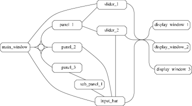
(b)

Figure 1: An example of confluent drawing of an object-interaction diagram. Nodes here denote components in a GUI program and edges indicate that the adjacent components send messages to each other. We show a standard drawing in (a) and a confluent drawing in (b).

In addition to providing heuristic algorithms for recognizing and drawing confluent diagrams, we also show that there are large classes of non-planar graphs that can be drawn in a planar way using our confluent diagram approach. For example, any interval graph or the complement of any tree can be visualized with a (planar) confluent diagram. Even so, we also show that there are unfortunately some graphs that cannot be drawn in a confluent way, including 4-dimensional hypercubes and a certain subgraph of the Petersen graph.

This paper is organized as follows. We give a formal definition of directed and undirected confluent diagrams in Section 2. We describe heuristic algorithms for recognizing and drawing directed and undirected confluent diagrams in Section 3. We show several special classes of confluently drawable graphs in Section 4, and in Section 5 we demonstrate several classes of graphs that cannot be drawn in a confluent way.

2 Confluent Drawings

It is well-known that every non-planar graph contains a subgraph homeomorphic to the complete graph on five vertices, $K_{5}$, or the complete bipartite graph between two sets of three vertices, $K_{3,3}$ (e.g., see [3, 20]). On the other hand, confluent drawings, with their ability to merge crossing edges into single tracks, can easily draw any $K_{n,m}$ or $K_{n}$ in a planar way. Figure. 2 shows confluent drawings of $K_{3,3}$ and $K_{5}$.

Figure 2: Confluent drawings of $K_{3,3}$ and $K_{5}$.

A curve is locally-monotone if it contains no self intersections and no sharp turns, that is, it contains no point with left and right tangents that form an angle less than or equal to $90$ degrees. Intuitively, a locally-monotone curve is like a single train track, which can make no sharp turns. Confluent drawings are a way to draw graphs in a planar manner by merging edges together into tracks, which are the unions of locally-monotone curves.

An undirected graph $G$ is confluent if and only if there exists a drawing $A$ such that:

• There is a one-to-one mapping between the vertices in $G$ and $A$, so that, for each vertex $v\in V(G)$, there is a corresponding vertex $v^{\prime}\in A$, which has a unique point placement in the plane.

• There is an edge $(v_{i},v_{j})$ in $E(G)$ if and only if there is a locally-monotone curve $e^{\prime}$ connecting $v_{i}^{\prime}$ and $v_{j}^{\prime}$ in $A$.

• $A$ is planar. That is, while locally-monotone curves in $A$ can share overlapping portions, no two can cross.

Our definition does not allow for confluent graphs to contain self loops or parallel edges, although we do allow for tracks to contain cycles and even multiple ways of realizing the same edge. Moreover, our definition implies that tracks in a confluent drawing have a “diode” property that does not allow one to double-back or make sharp turns after one has started going along a track in a certain direction.

(a)

(b)

Figure 3: A call graph (a) and its confluent drawing (b), with the dashed part showing the confluence.

Directed confluent drawings are defined similarly, except that in such drawings the locally-monotone curves are directed and the tracks formed by unions curves must be oriented consistently. Formally, a directed graph $D$ is confluent if and only if there exists a drawing $B$ such that

• There is a one-to-one mapping between the vertices in $D$ and $B$, so that, for each vertex $v\in V(D)$, there is a corresponding vertex $v^{\prime}\in B$, which has a unique point placement in the plane.

• There is an edge $(v_{i},v_{j})\in E(D)$ if and only if there is a locally-monotone curve $e^{\prime}$ connecting $v_{i}^{\prime}$ and $v_{j}^{\prime}$ in $B$.

• Locally-monotone curves in $B$ may share some overlapping portions, but the edges sharing the same portion of a track must all have the same direction along that portion.

• $B$ is directed and planar.

Figure 3 shows a part of the call graph of a Linux memory management module [14] and its corresponding confluent drawing. We choose this non-planar drawing to illustrate how confluent drawing works, and the level information of the drawing is still preserved. In the bottom figure we can easily tell the three functions (age_page_up, age_page_down, and zone_inactive_plenty) have two common callers
(refill_inactive_scan and try_to_swap_out), while in the original graph, it is a little more difficult to explore that information. One can imagine that confluent drawings can make complicated graphs more readable.

Confluent drawings remove crossings present in non-planar graphs, making the graphs’ structure easier to be understand. We feel that such drawings may also be helpful in discovering certain characteristic of the graphs. For example, given a confluent drawing, we can easily find the common source vertices and destination vertices of merged edges. Such common structures could indicate in a method-call diagram, say, separate methods that can be joined together for the sake of efficiency. Likewise, structures in which many sources all communicate with many destinations could indicate a need for refactoring or lead to other useful insights about a software design.

3 Heuristic Algorithms

Though the planarity of a graph can be tested in linear time, it appears difficult to quickly determine whether or not a graph can be drawn confluently. If a graph $G$ contains a non-planar subgraph, then $G$ itself is non-planar too. But similar closure properties are not true for confluent graphs. Adding vertices and edges to a non-confluent graph increases the chances of edges crossing each other, but it also increases the chances of edges merging. Currently, the best method we know of for determining conclusively in the worst case whether a graph is confluent or not is a brute force one of exhaustively listing all possible ways of edge merging and checking the merged graphs for planarity. Therefore, it is of interest to develop heuristics that can find confluent drawings in many cases.

Figure 4 shows confluent drawings using a “traffic circle” structure for complete graphs and complete bipartite subgraphs. At a high level, our heuristic drawing algorithm iteratively finds clique subgraphs and biclique subgraphs and replaces them with traffic-circle subdrawings.

Figure 4: Confluent drawings of $K_{5}$ and $K_{3,3}$ using “traffic circle” structures.

Chiba and Nishizeki [7] discuss the problem of listing complete subgraphs (cliques) for graphs of bounded arboricity. The arboricity $a(G)$ is the minimum number of forests into which the edges of $G$ can be partitioned. A bounded arboricity is equivalent to a notion of sparsity. We believe graphs arising in software visualization are often likely to be sparse, thus the listing algorithm is applicable for such graphs. Chiba and Nishizeki show that there can be at most $O(n)$ cliques of a given size in such graphs and give a linear time algorithm for listing these clique subgraphs. Eppstein [18] gives a linear time algorithm for listing maximal complete bipartite subgraphs (bicliques) in graphs of bounded arboricity. The total complexity of all such graphs is $O(n)$, and again they can be listed in linear time.

In our heuristic algorithm for undirected graphs, we will use the clique subgraphs listing and the biclique subgraphs listing algorithms as our subroutines.

HeuristicDrawUndirected($G$)
Input. A undirected sparse graph $G$.
Output. Confluent drawing of $G$ if succeed, fail otherwise.
1. If $G$ is planar
2.  draw $G$
3. else if $G$ contains a large clique or biclique subgraph $C$
4.  create a new vertex $v$
5.  obtain a new graph $G^{\prime}$ by removing edges of $C$ and connecting each vertex of $C$ to $v$
6.  HeuristicDrawUndirected($G^{\prime}$)
7.  replace $v$ by a small “traffic circle” to get a confluent drawing of $G$
8. else fail

In step 3, the cliques are given higher priority over bicliques, otherwise a clique would be partially covered by a biclique. Cliques of three or fewer vertices, and bicliques with one side consisting of only one vertex, are not replaced because the replacement cannot change the planarity of the graph. We now discuss the time performance of this heuristic.

Theorem 1

In graphs of bounded arboricity, algorithm HeuristicDrawUndirected can be made to run in time $O(n)$, assuming hash tables with constant time per operation.

Proof.

We store a bit per edge of the original graph so we can quickly look up whether it is still part of our replacement. We begin the heuristic by looking for cliques, since we want to give them priority over bicliques. List all the complete subgraphs in the graph with four or more vertices, and sort them by size. Then, for each complete subgraph $X$ in sorted order, we check whether $X$ is still a clique of the modified graph, and if so perform a replacement of $X$. It is not hard to see that the new vertex $v$ of the replacement cannot belong to any clique, so this algorithm correctly finds a maximal sequence of cliques to replace.

Next, we need to similarly dynamize the search for bicliques. This is more difficult, because a biclique may have nonconstant size and because the replacement vertex $v$ may belong to additional bicliques. We perform this step by dynamizing the algorithm of Eppstein [18] for listing all bicliques. This algorithm uses the idea of a $d$-bounded acyclic orientation: that is, an orientation of the edges of the graph, such that the oriented graph is acyclic and the vertices have maximum outdegree $d$. For graphs of arboricity $a$, a $(2a-1)$-bounded acyclic orientation may easily be found in linear time. For such an orientation, define a tuple to be a subset of the outgoing neighbors of any vertex, and let $v$ be a tuple creator of tuple $T$ if all vertices of $T$ are outgoing neighbors of $v$. For graphs of bounded arboricity, there are at most linearly many distinct tuples. For each maximal biclique, one of the two sides of the bipartition must be a tuple, $T$ [18]. The other side consists of two types of vertices: tuple creators of $T$, and outgoing neighbors of vertices of $T$.

Our algorithm stores a hash table indexed by the set of all tuples in the modified graph. The hash table entry for tuple $T$ stores the number of tuple creators of $T$, and a list of outgoing neighbors of vertices of $T$ that are adjacent to all tuple members. For each edge $(u,v)$ in the graph, oriented from $u$ to $v$, we store a list of the tuples $T$ containing $v$ for which $u$ is listed as an outgoing neighbor. We also store a priority queue of the maximal bicliques generated by each tuple, prioritized by size; it will suffice for our purposes if the time to find the largest biclique is proportional to the biclique size, and it is easy to implement a priority queue with such a time bound. With these structures, we may easily look up each successive biclique replacement to perform in algorithm HeuristicDrawUndirected. Each replacement takes time proportional to the number of edges removed from the graph, so the total time for performing replacements is linear.

It remains to show how to update these data structures when we perform a biclique replacement. To update the acyclic orientation, orient each edge from $C$ to $v$, except for those edges from vertices of $C$ that have no outgoing edges in $C$. It can be seen that this orientation preserves $d$-boundedness and acyclicity. When a new vertex $v$ is created by a replacement, create the appropriate hash table entries for tuples containing $v$; the number of tuples created by a replacement is proportional to the number of edges removed in the same replacement, so the total number of tuples created over the course of the algorithm is linear. Whenever a replacement causes edges from a vertex $x$ to change, update the hash entries for all tuples for which $x$ is a creator; this step takes $O(1)$ time per change. Also, update the hash entries for all tuples to which $x$ belongs, to remove vertices that are no longer outgoing neighbors of $x$; this step takes time $O(1)$ per changed tuple, and each tuple changes $O(1)$ times over the course of the algorithm. Whenever a change removes incoming edges of $x$, we must remove the other endpoints of those edges from the lists of outgoing neighbors of tuples to which $x$ belongs; using the lists associated with each incoming edge, this takes constant time per removal. Therefore, all steps can be performed in linear total time. ∎

An example of the input for algorithm HeuristicDrawUndirected and the output drawing produced by this heuristic is shown in Figure 5.

(a)

(b)

Figure 5: An example of running the undirected heuristic algorithm. The input graph is shown in (a) and the output drawing is shown in (b).

For directed graph, the algorithm is slightly different. Because the tracks in directed confluent drawings are required to have directions, the “traffic circle” structure will not work for directed cliques. Thus we only look for directed bicliques in step 3 in the directed version of the heuristic algorithm. Next we discuss how to find maximal directed bicliques. Maximal directed complete bipartite subgraphs in a sparse directed graph $G$ can be found by first listing maximal undirected complete bipartite subgraphs in the underlying undirected graph of $G$. Then for each of these subgraphs examine the corresponding directed subgraph. We choose the side of the bipartition with larger size and partition it according to how their edges are oriented to the other side of the bipartition (In Figure 6, the bottom directed $K_{3,4}$ is obtained from the top graph).

Figure 6: Maximal directed complete bipartite subgraphs.

4 Some Confluent Graphs

The heuristic algorithms presented in the previous section are most applicable to sparse graphs, because sparseness is needed for the linear time bound of the maximal bipartite subgraph listing subroutine. However, there are also several denser classes of graphs that we can show to be confluent.

4.1 Interval graphs

An interval graph is formed by a set of closed intervals $S=\{[a_{1},b_{1}],[a_{2},b_{2}],\ldots,[a_{n},b_{n}]\}$. The interval graph is defined to have the intervals in $S$ as its vertices and two vertices $[a_{i},b_{i}]$ and $[a_{j},b_{j}]$ are connected by an edge if and only if these two inverals have a non-empty intersection. Such graphs are typically non-planar, but we can draw them in a planar way using a confluent drawing.

Theorem 2

Every interval graph is confluent.

Proof.

The proof is by construction. We number the interval endpoints by rank, $X=\{0,1,\ldots,n-1\}$, and place these endpoints along the $x$-axis. We then build a two-dimensional lattice on top of these points in a fashion similar to Pascal’s triangle, using a connector similar to an upside-down “V”. These connectors stack on top of one another so that the apex of each is associated with a unique interval on $X$. We place each point from our set $S$ of intervals just under its corresponding apex and connect it into the (single) track so that it can reach everything directly dominated by this apex in the lattice. At the bottom level, we connect the updside-down V’s with rounded connectors. By this contruction, we create a single track that allows each pair of vertices connected in the interval graph to have a locally-monotone path connecting them. (See Figure 7.) ∎∎

(a)

(b)

Figure 7: Illustrating a confluent way to draw a non-planar interval graph: (a) an interval garph and its defining intervals; (b) its corresponding confluent drawing.

4.2 Complements of trees

The complements of trees (graphs formed by connecting all pairs of vertices that are not connected in some tree) are also called cotrees. In general, cotrees are highly non-planar and dense, since a cotree with $n$ vertices has $n(n-1)/2-n+1$ edges. Nevertheless, we have the following interesting fact.

Theorem 3

The complement of a tree is confluent.

Proof.

We prove the claim by recursive construction, using a single track for the entire graph. Assign a bounding rectangle for the tree and a bounding rectangle for every subtree in that tree. Place the complement of the tree into the bounding rectangles such that nodes of every subtree is within its bounding rectangle and the bounding rectangles of subtrees are contained in their parent’s bounding rectangle. In addition, place a connector at the Northeastern corner of every bounding box. This connector is an imaginary point at which the single track for the entire graph will connect into this portion of the cotree. (See Figure 8.) Connect the root node in each subtree to every connector of its children. Connect every node to the connector of its parent. Also connect every node to its siblings and the connectors of its siblings, as shown in the figure. The obtained drawing is the confluent drawing of the complement of the given tree. ∎∎

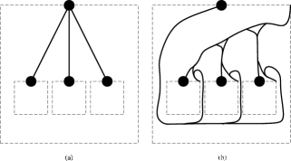
Figure 8: Illustrating a confluent way to draw the complement of a tree: (a) a node and its children in the tree; (b) the corresponding portion of a track in the confluent drawing of the complement.

Paths are very special cases of trees. Every vertex in a path has a degree of $2$ except its two endpoints, each of which has a degree of $1$. The complement of a path can be drawn using the cotree method in the above proof. We show a nice confluent drawing of the complement of a path in Figure 9.

Figure 9: A path and one confluent drawing of its complement.

4.3 Cographs

A complement reducible graph (also called a cograph) is defined recursively as follows [12]:

• A graph on a single vertex is a cograph.

• If $G_{1}$, $G_{2}$, $\cdots$, $G_{k}$ are complement reducible graphs, then so is their union $G_{1}\cup G_{2}\cup\cdots\cup G_{k}$.

• If $G$ is a complement reducible graph, then so is its complement $\overline{G}$.

Cographs can be obtained from single node graphs by performing a finite number of unions and complementations.

Theorem 4

Cographs are confluent.

Proof.

If cographs $A$ and $B$ are confluent, we can show $A\cup B$ and $\overline{A\cup B}$ are confluent too. First we draw $A$ confluently inside a disk and attach a “tail” to the boundary of the disk. Connect the attachment point to each vertex in the disk. $B$ is drawn in the same way. Then $A\cup B$ is formed by joining the two “tail” together so that they don’t connect to each other. $\overline{A\cup B}$ is formed by joining the two “tails” of $\overline{A}$ and $\overline{B}$ together so that they connect to each other. (See Figure 10.) By the definition of cographs and induction we know cographs are confluent. ∎∎

Figure 10: Confluent $A\cup B$ and $\overline{A\cup B}$.

(a)

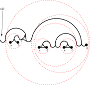
(b)

Figure 11: Confluent drawing of a cograph $\overline{\cup}(\overline{\cup}(a,b),\overline{\cup}(\overline{\cup}(c,d),\overline{\cup}(e,f),g))$. Imaginary disks are drawn in dashed circle.

4.4 Complements of $n$-cycles

A $n$-cycle is a cycle with $n$ vertices.

Theorem 5

The complement of an $n$-cycle is confluent.

Proof.

First remove one vertex from the $n$-cycle and draw the confluent graph for the complement of the obtained path. Then add the vertex back and connect it with all vertices in the path except for its two neighbors. The obtained drawing is a confluent drawing. ∎∎

An example of drawing a cocycle confluently is shown in Figure 12.

Figure 12: A confluent drawing of $\overline{C}_{8}$.

5 Some Non-confluent Graphs

In this section, we show that some graphs cannot be drawn confluently. These graphs include the Peterson graph $P$, the graph $P-v$ formed by removing one vertex from Peterson graph, graphs formed by subdividing every edge of non-planar graphs, and the $4$-dimensional hypecube.

5.1 The Petersen graph

By removing one vertex and its incident edges from the Petersen graph (Figure 13) we obtain a graph homeomorphic to $K_{3,3}$. It contains no $K_{2,2}$ as a subgraph. Moreover, note that $K_{2,2}$ is the most basic structure that allows for edge merging into tracks. Thus the resulting graph is non-confluent. This graph, shown in Figure 14, is the smallest non-confluent graph we know of.

Figure 13: The Petersen graph. The edges incident on one of the vertices are shown dashed.

Figure 14: Removing one vertex of the Petersen graph produces a subdivision of $K_{3,3}$.

The Petersen graph itself is also non-confluent, as adding the vertex and edges back to its non-confluent subgraph doesn’t create any four-cycles that could be used for confluent tracks.

5.2 Other non-confluent graphs

If we subdivide every edge of a non-planar graph, by adding a single vertex in the “middle” of each edge, the resulting graph is non-confluent, because the new vertices do not take part in any 4-cycles and so can not be included in any confluent tracks. For the same reason, if, for each edge of a non-planar graph, we add a new vertex and connect this new vertex to the both end points of that edge, the result is also non-confluent. In particular, adding new vertices in this way to the graph $K_{5}$ produces a non-confluent chordal graph, so despite our proofs that other graph families with tree-like structures are confluent, chordal graphs are not all confluent.

5.3 4-dimensional cube

The $4$-dimensional hypercube in Figure 15 (a) is non-confluent.

Figure 15: The $4$-dimensional hypercube.

The hypercube contains many subgraphs isomorphic to $3$-dimensional cubes. Cubes are planar graphs, but in order to show non-confluence for the hypercube, we analyze more carefully the possible drawings of the cubes. Observe that, because there are no $K_{2,3}$ subgraphs in cubes or hypercubes, the only possible confluent tracks are $K_{2,2}$’s formed from the vertices of a single cube face.

$${\includegraphics[scale={.4}]{cube4}\atop\hbox{(a)}}\hbox{\hskip 10.0pt}{\includegraphics[scale={.4}]{cube3}\atop\hbox{(b)}}\hbox{\hskip 10.0pt}{\includegraphics[scale={.4}]{cube5}\atop\hbox{(c)}}\hbox{\hskip 10.0pt}$$

Figure 16: Three confluent drawings of a cube.

Lemma 1

A cube has only the four confluent drawings shown in Figure 16, or combinatorially equivalent rearrangements of these drawings in which we choose a different face as the outer one.

Proof.

For convenience, we consider the drawings to be on a sphere instead of in the plane, so the outer face is not distinguished. Every cube face can be drawn either as a quadrilateral or as a track in a confluent drawing of $K_{2,2}$. We divide into cases based on the number of cube faces replaced by tracks.

Case 0: No faces are replaced by tracks. We get the usual planar drawing of a cube. It is unique because a cube is $3$-connected.

Case 1: One face is replaced by a track. This case is not possible, because the underlying graph of the drawing (formed by placing new vertices at track junctions) is non-planar.

Case 2: Only two adjacent faces are replaced by tracks. We have the drawing of Figure 16 (a). It is unique because the underlying planar graph is $3$-connected.

Case 3: Two opposite faces are replaced by tracks. We have the drawing of Figure 16 (b). It is unique because the underlying planar graph is $3$-connected.

Case 4: Three mutually adjacent faces are replaced by tracks. This case is not possible, even if we allow additional faces to be replaced by tracks as well. For, suppose the faces $0-1-3-2$, $0-2-6-4$, and $0-1-5-4$ are replaced by tracks. The underlying graph of these replaced edges has a drawing with four faces, in which vertices $3$, $5$, and $6$ are dangling and may each go in either of two faces (Figure 17). However, it is not possible for all three to be in the same face. So they can’t all three be connected to vertex $7$, as edges to $7$ can not cross the existing tracks.

Figure 17: Attempt to use confluent tracks for three mutually-adjacent faces of a cube.

Case 5: Three non-mutually adjacent faces are replaced by tracks. This case is not possible because the underlying graph is non-planar (Figure 18).

Figure 18: Attempt to use confluent tracks for three non-mutually-adjacent faces of a cube.

Case 6: A ring of four faces are replaced by tracks. We have the drawing of Figure 16 (c). It is unique too.

There are no other cases left. Thus a cube only has four confluent drawings. ∎

Theorem 6

The hypercube is non-confluent.

Proof.

If we have a valid confluent drawing of the hypercube, and choose eight of its vertices in the form of a cube, the portion of the drawing connecting these vertices must be in one of the forms listed in the lemma above. We consider the four possible drawings of this cube, and attempt to add the other eight vertices (which also form a cube), showing that each case leads to a contradiction. Note that, among the edges of the first cube’s drawing, only the ones drawn as single edges can take part in confluent tracks with the remaining eight vertices.

Case 0: In this drawing no faces are replaced. Since the hypercube is non-planar, at least one of its faces must be replaced, so we can always choose our first cube in such a way that this case does not occur.

Case 1: Two adjacent faces of the cube are replaced, as in Figure 16 (a). If only two adjacent faces $f_{1}$ and $f_{2}$ of the cube $C_{1}$ are replaced by tracks, find a different cube $C_{2}$ sharing $f_{1}$ but not $f_{2}$ with $C_{1}$. $C_{2}$ must have a second replaced face $f_{3}$ (it not possible for a cube to have a confluent drawing with only one face replaced). Either $f_{1}-f_{3}$ and $f_{2}-f_{3}$ are non-adjacent faces of the same cube. So if this case exists, we can find a different cube that is in case 2 or case 3.

Case 3: Two opposite faces of the cube are replaced, as in Figure 16 (b). In this drawing, each face of the cube has only two non-track edges, each of which can be crossed by at most one edge from the rest of the graph. Because the other eight vertices of the graph form a cube which is $3$-connected, any subset of these eight vertices has more than two edges connecting to the complement of the subset. So putting any subset of these vertices, other than the whole set, in a single face of the cube drawing does not work. Putting the whole set of the remaining vertices in a single face of the cube drawing does not work either because there are four vertices of the first cube outside that single face to be reached, and only two of them can be reached across the two non-track edges.

Case 4: A ring of four faces of the cube are replaced, as in Figure 16 (c). Edges between the other eight vertices can not cross the tracks, so these vertices must all be placed within a single face of the first cube’s drawing. However, these vertices would then be unable to connect to the four or more vertices of the first cube outside that face.

Since all cases fail, the $4$-dimensional hypercube is non-confluent. ∎

6 Conclusions

We introduce a new method of drawing non-planar graphs in planar way. This can be very helpful for drawing graphs in the area of Software Visualization. Though we only show its applications on drawing function call graphs and object-interaction graphs, it is powerful for visualizing other kinds of graphs too.

Acknowledgments

We would like to thank Jie Ren and André van der Hoek for supplying us with several examples of graphs used in software visualization. David Eppstein’s research was supported by NSF grant CCR-9912338.

References

- [1] T. Ball and S. G. Eick. Software visualization in the large. IEEE Computer, 29(4):33–43, 1996.
- [2] C. Batini, E. Nardelli, and R. Tamassia. A layout algorithm for data flow diagrams. IEEE Trans. Softw. Eng., SE-12(4):538–546, 1986.
- [3] J. A. Bondy and U. S. R. Murty. Graph Theory with Applications. Macmillan, London, 1976.
- [4] G. Booch. Object-Oriented Analysis and Design with Applications. Benjamin/Cummings, 2 edition, 1994.
- [5] R. Breu, U. Hinkel, C. Hofmann, C. Klein, B. Paech, B. Rumpe, and V. Thurner. Towards a formalization of the unified modeling language. In Proc. 11th European Conf. Object-Oriented Programming (ECOOP’97), volume 1241 of Lecture Notes in Computer Science, pages 344–366, 1997.
- [6] C. C. Cheng, C. A. Duncan, M. T. Goodrich, and S. G. Kobourov. Drawing planar graphs with circular arcs. In Proc. Graph Drawing, volume 1731 of Lecture Notes in Computer Science, pages 117–126, 1999.
- [7] N. Chiba and T. Nishizeki. Arboricity and subgraph listing algorithms. SIAM J. Comput., 14:210–223, 1985.
- [8] N. Chiba, T. Nishizeki, S. Abe, and T. Ozawa. A linear algorithm for embedding planar graphs using PQ-trees. J. Comput. Syst. Sci., 30(1):54–76, 1985.
- [9] N. Chiba, K. Onoguchi, and T. Nishizeki. Drawing planar graphs nicely. Acta Inform., 22:187–201, 1985.
- [10] N. Chiba, T. Yamanouchi, and T. Nishizeki. Linear algorithms for convex drawings of planar graphs. In J. A. Bondy and U. S. R. Murty, editors, Progress in Graph Theory, pages 153–173. Academic Press, New York, NY, 1984.
- [11] M. Chrobak and T. H. Payne. A linear time algorithm for drawing a planar graph on a grid. Technical Report UCR-CS-90-2, Dept. of Math. and Comput. Sci., Univ. California Riverside, 1990.
- [12] D. G. Corneil, H. Lerchs, and L. S. Burlingham. Complement reducible graphs. Discrete Appl. Math., 3:163–174, 1981.
- [13] H. de Fraysseix, J. Pach, and R. Pollack. How to draw a planar graph on a grid. Combinatorica, 10(1):41–51, 1990.
-
[14]
M. Devera.
http://luxik.cdi.cz/
~devik/mm.htm. - [15] G. Di Battista, P. Eades, R. Tamassia, and I. G. Tollis. Graph Drawing. Prentice Hall, Upper Saddle River, NJ, 1999.
- [16] D. Dolev, F. T. Leighton, and H. Trickey. Planar embedding of planar graphs. In F. P. Preparata, editor, VLSI Theory, volume 2 of Adv. Comput. Res., pages 147–161. JAI Press, Greenwich, Conn., 1984.
- [17] P. Eades and P. Mutzel. Graph drawing algorithms. In M. Atallah, editor, CRC Handbook of Algorithms and Theory of Computation, chapter 9. CRC Press, 1999.
- [18] D. Eppstein. Arboricity and bipartite subgraph listing algorithms. Information Processing Letters, 51(4):207–211, August 1994.
- [19] M. R. Garey and D. S. Johnson. Crossing number is NP-complete. SIAM J. Algebraic Discrete Methods, 4(3):312–316, 1983.
- [20] A. Gibbons. Algorithmic Graph Theory. Cambridge University Press, Cambridge, 1985.
- [21] M. T. Goodrich and C. G. Wagner. A framework for drawing planar graphs with curves and polylines. J. Algorithms, 37:399–421, 2000.
- [22] D. Grove, G. DeFouw, J. Dean, and C. Chambers. Call graph construction in object-oriented languages. In Proc. of ACM Symp. on Object-Oriented Prog. Sys., Lang. and Applications (OOPSLA), pages 108–124, 1997.
- [23] C. Gutwenger and P. Mutzel. Planar polyline drawings with good angular resolution. In Graph Drawing (Proc. GD 98), volume 1547 of Lecture Notes in Computer Science, pages 167–182, 1998.
- [24] P. Haynes, T. J. Menzies, and R. F. Cohen. Visualisations of large object-oriented systems. In P. D. Eades and K. Zhang, editors, Software Visualisation, volume 7, pages 205–218. World Scientific, Singapore, 1996.
- [25] M. Jünger, E. K. Lee, P. Mutzel, and T. Odenthal. A polyhedral approach to the multi-layer crossing minimization problem. In G. Di Battista, editor, Graph Drawing (Proc. GD ’97), number 1353 in Lecture Notes Comput. Sci., pages 13–24. Springer-Verlag, 1997.
- [26] M. Jünger and P. Mutzel. 2-layer straightline crossing minimization: Performance of exact and heuristic algorithms. J. Graph Algorithms Appl., 1(1):1–25, 1997.
- [27] G. Kant. Drawing planar graphs using the canonical ordering. Algorithmica, 16:4–32, 1996. (special issue on Graph Drawing, edited by G. Di Battista and R. Tamassia).
- [28] M. Kaufmann and D. Wagner. Drawing Graphs: Methods and Models, volume 2025 of Lecture Notes in Computer Science. Springer-Verlag, 2001.
- [29] D. E. Knuth. Computer drawn flowcharts. Commun. ACM, 6, 1963.
- [30] P. Mutzel. An alternative method to crossing minimization on hierarchical graphs. In S. North, editor, Graph Drawing (Proc. GD ’96), volume 1190 of Lecture Notes Comput. Sci., pages 318–333. Springer-Verlag, 1997.
- [31] P. Mutzel and T. Zeigler. The constrained crossing minimization problem. In J. Kratochvil, editor, Graph Drawing Conference, volume 1731 of Lecture Notes in Computer Science, pages 175–185. Springer-Verlag, 1999.
- [32] T. Nishizeki and N. Chiba. Planar Graphs: Theory and Algorithms, volume 32 of Ann. Discrete Math. North-Holland, Amsterdam, The Netherlands, 1988.
- [33] R. C. Penner and J. L. Harer. Combinatorics of Train Tracks, volume 125 of Annals of Mathematics Studies. Princeton Univ. Press, Princeton, NJ, 1992.
- [34] B. Price, R. Baecker, and I. Small. A principled taxonomy of software visualization. Journal of Visual Languages and Computing, 4(3):211–266, 1993.
- [35] H. Purchase. Which aesthetic has the greatest effect on human understanding? In G. Di Battista, editor, Proc. 5th Int. Symp. Graph Drawing, GD, number 1353 in Lecture Notes in Computer Science, LNCS, pages 248–261. Springer-Verlag, 18–20 Sept. 1997.
- [36] G.-C. Roman and K. C. Cox. A taxonomy of program visualization systems. IEEE Computer, 26(12):11–24, 1993.
- [37] J. Rumbaugh, I. Jacobson, and G. Booch. The Unified Modeling Language Reference Manual. Addison-Wesley, 1998.
- [38] W. Schnyder. Embedding planar graphs on the grid. In Proc. 1st ACM-SIAM Sympos. Discrete Algorithms, pages 138–148, 1990.
- [39] J. T. Stasko and E. Kraemer. A methodology for building application-specific visualizations of parallel programs. Journal of Parallel and Distributed Computing, 18(2):258–264, 1993.
- [40] R. Tamassia and I. G. Tollis. Planar grid embedding in linear time. IEEE Trans. Circuits Syst., CAS-36(9):1230–1234, 1989.
- [41] F. Tip and J. Palsberg. Scalable propagation-based call graph construction algorithms. ACM SIGPLAN Notices, 35(10):281–293, 2000.