Solving a “Hard” Problem to Approximate an “Easy” One: Heuristics for Maximum Matchings and Maximum Traveling Salesman Problems

Abstract

We consider geometric instances of the Maximum Weighted Matching Problem (MWMP) and the Maximum Traveling Salesman Problem (MTSP) with up to 3,000,000 vertices. Making use of a geometric duality relationship between MWMP, MTSP, and the Fermat-Weber-Problem (FWP), we develop a heuristic approach that yields in near-linear time solutions as well as upper bounds. Using various computational tools, we get solutions within considerably less than 1% of the optimum.

An interesting feature of our approach is that, even though an FWP is hard to compute in theory and Edmonds’ algorithm for maximum weighted matching yields a polynomial solution for the MWMP, the practical behavior is just the opposite, and we can solve the FWP with high accuracy in order to find a good heuristic solution for the MWMP.

An extended abstract appears in the proceedings of ALENEX’01 [Fekete et al. (2001)].

1 Introduction

1.1 Complexity in Theory and Practice

In the field of discrete algorithms, the classical way to distinguish “easy” and “hard” problems is to study their worst-case behavior. Ever since Edmonds’ seminal work on maximum matchings [Edmonds (1965b), Edmonds (1965a)], the adjective “good” for an algorithm has become synonymous with a worst-case running time that is bounded by a polynomial in the input size. At the same time, Edmonds’ method for finding a maximum weight perfect matching in a complete graph with edge weights serves as a prime example for a sophisticated combinatorial algorithm that solves a problem to optimality. Furthermore, finding an optimal matching in a graph is used as a stepping stone for many heuristics for hard problems.

The classical prototype of such a “hard” problem is the Traveling Salesman Problem (TSP) of computing a shortest roundtrip through a set $P$ of $n$ cities. Being NP-hard, it is generally assumed that there is no “good” algorithm in the above sense: Unless P=NP, there is no polynomial-time algorithm for the TSP. This motivates the performance analysis of polynomial-time heuristics for the TSP. Assuming triangle inequality, the best polynomial heuristic known to date uses the computation of an optimal weighted matching: Christofides’ method combines a Minimum Weight Spanning Tree (MWST) with a Minimum Weight Perfect Matching of the odd degree vertices, yielding a worst-case performance of 50% above the optimum.

1.2 Geometric Instances

Virtually all very large instances of graph optimization problems are geometric. It is easy to see why this should be the case for practical instances. In addition, a geometric instance given by $n$ vertices in ${I\!\!R}^{d}$ is described by only $dn$ coordinates, while a distance matrix requires $\Omega(n^{2})$ entries; even with today’s computing power, it is hopeless to store and use the distance matrix for instances with, say, $n=10^{6}$.

The study of geometric instances has resulted in a number of powerful theoretical results. Most notably, Arora 1998 and Mitchell 1999 have developed a general framework that results in polynomial-time approximation schemes (PTASs) for many geometric versions of graph optimization problems: Given any constant $\epsilon$, there is a polynomial algorithm that yields a solution within a factor of $(1+\epsilon)$ of the optimum. However, these breakthrough results are of purely theoretical interest, because the necessary computations and data storage requirements are beyond any practical orders of magnitude.

For a problem closely related to the TSP, there is a different way how geometry can be exploited. Trying to find a longest tour in a weighted graph is the so-called Maximum Traveling Salesman Problem (MTSP); it is straightforward to see that for graph instances, the MTSP is just as hard as the TSP: replace the weight $c_{e}$ of any edge $e$ by $M-c_{e}$, for a sufficiently big $M$. Making clever use of the special geometry of distances, Barvinok, Johnson, Woeginger, and Woodroofe 1998 showed that for geometric instances in ${I\!\!R}^{d}$, it is possible to solve the MTSP in polynomial time, provided that distances are measured by a polyhedral metric, which is described by a unit ball with a fixed number $2f$ of facets. (For the case of Manhattan distances in the plane, we have $f=2$, and the resulting complexity is $O(n^{2f-2}\log n)=O(n^{2}\log n)$.) By using a large enough number of facets to approximate a unit sphere, this yields a PTAS for Euclidean distances.

Both of these approaches, however, do not provide practical methods for getting good solutions for very large geometric instances. And even though TSP and matching instances of considerable size have been solved to optimality (up to 13,509 cities with about 10 years of computing time Applegate et al. (1998)), it should be stressed that for large enough instances, it seems quite difficult to come up with fast (i.e., near-linear in $n$) solution methods that find good solutions that leave only a provably small gap to the optimum. Moreover, the methods involved only use triangle inequality, and disregard the special properties of geometric instances.

For the Minimum Weight Matching problem, Vaidya (1989) showed that there is algorithm of complexity $O(n^{2.5}\log^{4}n)$ for planar geometric instances, which was improved by Varadarajan (1998) to $O(n^{1.5}\log^{5}n)$. Cook and Rohe (1999) also made heavy use of geometry to solve instances with up to 5,000,000 points in the plane within about 1.5 days of computing time. However, all these approaches use specific properties of planar nearest neighbors. Cook and Rohe reduce the number of edges that need to be considered to about 8,000,000, and solve the problem in this very sparse graph. These methods cannot be applied when trying to find a Maximum Weight Matching. (In particular, a divide-and-conquer strategy seems unsuited for this type of problem, because the structure of furthest neighbors is quite different from the well-behaved “clusters” formed by nearest neighbors.)

1.3 Heuristic Solutions

A standard approach when considering “hard” optimization problems is to solve a closely related problem that is “easier”, and use this solution to construct one that is feasible for the original problem. In combinatorial optimization, finding an optimal perfect matching in an edge-weighted graph is a common choice for the easy problem. However, for practical instances of matching problems, the number $n$ of vertices may be too large to find an exact optimum in reasonable time, as the fastest exact algorithm still has a complexity of $O(n(m+n\log n))$ Gabow (1990) (where $m$ is the number of edges).

We have already introduced the Traveling Salesman Problem, which is known to be NP-hard, even for geometric instances. A problem that is hard in a different theoretical sense is the following: For a given set $P$ of $n$ points in ${I\!\!R}^{2}$, the Fermat-Weber Problem (FWP) is to minimize the size of a “Steiner star”, i.e., the total Euclidean distance $S(P)=\min_{c\in{I\!\!R}}\sum_{p\in P}d(c,p)$ of a point $c$ to all points in $P$. It was shown in Bajaj (1988) that even for the case $n=5$, solving this problem requires finding zeroes of high-order polynomials, which cannot be achieved using only radicals. In particular, this implies that there is no “clean” geometric solution that uses only ruler and compass. Since the ancient time of Greek geometry, the latter has been considered superior to other solution methods. Even in modern times, purely numerical methods are considered inferior by many mathematicians. One important reason can actually be understood by considering a modern piece of software like Cinderella Richter-Gebert and Kortenkamp (1999): In this feature-based geometry tool, objects can be defined by the relations of other geometric objects. Interactively and dynamically changing one of the defining objects causes an automatic and continuous update of the other objects. Obviously, this is much harder if the dependent object can only be computed numerically.

Solving instances of the FWP and of the geometric maximum weight matching problem (MWMP) are closely related. Let $\mbox{FWP}(P)$ and $\mbox{MWMP}(P)$ denote the cost of an optimal solution of the FWP and the MWMP for a given point set $P$. It is an easy consequence of the triangle inequality that $\mbox{MWMP}(P)\leq\mbox{FWP}(P)$, as any edge of a matching is at most as long as a connection via a central point $c$. For a natural geometric case of Euclidean distances in the plane, it was shown in Fekete and Meijer (2000) that FWP(P)/${{\mbox{MWMP}}{\mbox{\em(P)}}}\leq{2}/{\sqrt{3}}\approx 1.15$.

From a theoretical point of view, this may appear to assign the roles of “easy” and “hard” to MWMP and FWP. However, from a practical perspective, roles are reversed: While solving large maximum weight matching problems to optimality seems like a hopeless task, finding an optimal Fermat-Weber point $c$ only requires minimizing a convex function. Thus, the latter can be solved very fast numerically (e.g., by Newton’s method) within any small $\varepsilon$. The twist of this paper is to use that solution to construct a fast heuristic for maximum weight matchings – thereby solving a “hard” problem to approximate an “easy” one. Similar ideas can be used for constructing a good heuristic for the MTSP.

1.4 Summary of Results

It is the main objective of this paper to demonstrate that the special properties of geometric instances can make them much easier in practice than general instances on weighted graphs. Using these properties gives rise to heuristics that construct excellent solutions in near-linear time, with very small constants. We will show that weak approximations of $\mbox{FWP}(P)$ can be used to construct approximations of $\mbox{MWMP}(P)$ that are within a factor $2/\sqrt{3}\approx 1.15$ of the optimal answers. By using a stronger approximations of $\mbox{FWP}(P)$ we obtain approximations of $\mbox{MWMP}(P)$ that in practice are much closer to the optimal solutions.

1. This is validated by a practical study on instances up to 3,000,000 points, which can be dealt with in less than three minutes of computation time, resulting in error bounds of not more than about 3% for one type of instances, but only in the order of 0.1% for most others. The instances consist of the well-known TSPLIB Reinelt (1991), and random instances of two different random types, uniform random distribution and clustered random distribution.

2. We can also use an approximation of the FWP to obtain an approximate answer of the MTSP. Let $\mbox{MTSP}(P)$ denote the cost of an optimal solution of the MTSP for a given point set $P$. The worst-case estimate for the ratio between $\mbox{MTSP}(P)$ and 2FWP($P$) is slightly worse than the one between $\mbox{MWMP}(P)$ and $\mbox{FWP}(P)$. We describe an instance for which

   $2\mbox{FWP}(P)/\mbox{MTSP}(P)=4/(2+\sqrt{2})\approx 1.17>1.15\approx 2/\sqrt{3}\geq\mbox{FWP}(P)/\mbox{MWMP}(P)$

   holds. However, we show that for large $n$, the asymptotic worst-case performance for the $\mbox{MTSP}(P)$ is the same as for $2\mbox{MWMP}(P)$. We will show that the worst-case gap for our heuristic is asymptotically bounded by 15%, and not by 17%, as suggested by the above example.

3. For a planar set of points that are sorted in convex position (i.e., the vertices of a polyhedron in cyclic order), we can solve the MWMP and the MTSP in linear time.

To evaluate the quality of our results for both MWMP and MTSP, we employ a number of additional methods, including the following:

1. An extensive local search by use of the chained Lin-Kernighan method (see Rohe (1997)) yields only small improvements of our heuristic solutions. This provides experimental evidence that a large amount of computation time will only lead to marginal improvements of our heuristic solutions.

2. An improved upper bound (that is more time-consuming to compute) indicates that the remaining gap between the fast feasible solutions and the fast upper bounds is too pessimistic on the quality of the heuristic, because the gap seems to be mostly due to the difference between the optimum and the upper bound.

3. A polyhedral result on the structure of optimal solutions to the MWMP allows the computation of the exact optimum by using a network simplex method, instead of employing Edmonds’ blossom algorithm. This result (stating that there is always an integral optimum of the standard LP relaxation for planar geometric instances of the MWMP) is interesting in its own right and was observed by Tamir and Mitchell (1998). A comparison for instances with less than 10,000 nodes shows that the gap between the solution computed by our heuristic and the upper bound derived from $\mbox{FWP}(P)$ is much larger than the difference between our solution and the actual optimal value of $\mbox{MWMP}(P)$, which turns out to be at most 0.26%, even for clustered instances. Moreover, twice the optimum solution for the MWMP is also an upper bound for the MTSP. For both problems, this provides more evidence that additional computing time will almost entirely be used for lowering the fast upper bound on the maximization problem, while the feasible solution changes only little.

4. We compare the feasible solutions and bounds for our MTSP heuristic with an “exact” method that uses the existing TSP package Concorde for TSPLIB instances of moderate size (up to about 1000 points). It turns out that almost all our results lie within the widely accepted margin of error caused by rounding distances to the nearest integer. Furthermore, the (relatively time-consuming) standard Held-Karp bound (see Held and Karp (1971)) is outperformed by our methods for most instances. This is remarkable, as it usually performs quite well, and has been studied widely, even for geometric instances of the TSP. (See Valenzuela and Jones (1997).)

2 Minimum Stars and Maximum Matchings

2.1 Background and Algorithm

Consider a set $P$ of points in ${I\!\!R}^{2}$ of even cardinality $n$. The Fermat-Weber Problem (FWP) is given by minimizing the total Euclidean distance of a “median” point $c$ to all points in $P$, i.e., $\mbox{FWP}(P)=\min_{c\in R}\sum_{p\in P}d(c,p)$. This problem cannot be solved to optimality by methods using only radicals, because it requires to find zeroes of high-order polynomials, even for instances that are symmetric around the $y$-axis; see Bajaj (1988). In Fekete and Meijer (2000) it is shown that given a planar point set, a point $c$ can be found and a subdivision of the plane into six sectors of $\pi/3$ around $c$, such that opposite sectors have the same number of points. An approximation of the FWP can be found by using this point $c$. We denote the approximate value of the FWP for a given point set $P$ using this combinatorial method by $\mbox{FWP}_{com}(P)$. The objective function of the FWP is strictly convex, so it is possible to solve the problem numerically with any required amount of accuracy. A simple binary search will do, but there are more specific approaches like the so-called Weiszfeld iteration Kuhn (1973); Weiszfeld (1937). We achieved the best results by using Newton’s method. We denote the approximate value using this method by $\mbox{FWP}_{num}(P)$. By starting the numeric approximation with the combinatorial approximation, we get $\mbox{FWP}(P)\leq\mbox{FWP}_{num}(P)\leq\mbox{FWP}_{com}(P)$.

Figure 1: Angles and rays for a matching edge $(p_{i},p_{j})$.

The relationship between the FWP and the MWMP for a point set of even cardinality $n$ has been studied in Fekete and Meijer (2000): Any matching edge between two points $p_{i}$ and $p_{j}$ can be mapped to two “rays” $(c,p_{i})$ and $(c,p_{j})$ of the star, so it follows from the triangle inequality that $\mbox{MWMP}(P)\leq\mbox{FWP}(P)$.

Let $c$ be the center of $\mbox{FWP}_{com}(P)$ for a given point set $P$. Assume we sort $P$ by angular order around $c$. Assume the resulting order is $p_{1},p_{2},\ldots,p_{n}$. Let $\mbox{MWMP}_{com}(P)$ be the cost of the approximate maximal matching that is obtained b matching $p_{i}$ with $p_{i+n/2}$. The ratio between the values $\mbox{MWMP}_{com}(P)$ and $\mbox{FWP}_{com}(P)$ depends on the amount of “shortcutting” that happens when replacing pairs of rays by matching edges; moreover, any lower bound for the angle $\varphi_{ij}$ between the rays for a matching edge is mapped directly to a worst-case estimate for the ratio, because it follows from elementary trigonometry that $d(c,p_{i})+d(c,p_{j})\leq\sqrt{\frac{2}{1-\cos\varphi_{ij}}}\cdot d(p_{i},p_{j})$. See Fig. 1. It was shown in Fekete and Meijer (2000) that for $\mbox{MWMP}_{com}(P)$ we have $\varphi_{ij}\geq 2\pi/3$ for all angles $\varphi_{ij}$ between rays. It follows that $\mbox{FWP}_{com}(P)\leq\mbox{MWMP}_{com}(P)\cdot 2/\sqrt{3}$. So we have $\mbox{MWMP}_{com}(P)\leq\mbox{MWMP}(P)\leq\mbox{MWMP}_{com}(P)\cdot 2/\sqrt{3}$.

Algorithm CROSS: Heuristic solution for MWMP Input: A set of points $P\in{I\!\!R}^{2}$. Output: A matching of $P$. 1. Using a numerical method, find a point $c$ that approximately minimizes the convex function $\min_{c\in{I\!\!R}^{2}}\sum_{p_{i}\in P}d(c,p_{i})$. 2. Sort the set $P$ by angular order around $c$. Assume the resulting order is $p_{1},\ldots,p_{n}$. 3. For $i=1,\ldots,n/2$, match point $p_{i}$ with point $p_{i+n/2}$.

Figure 2: The heuristic CROSS.

If we use a better approximation for the center of the FWP, we expect to get a better estimate for the value of the matching. This motivates the heuristic CROSS for large-scale MWMP instances that is shown in Fig. 2. See Fig. 3 for a heuristic solution for the 100-point instance TSPLIB instance dsj1000. Let $\mbox{MWMP}_{num}(P)$ denote the value of the matching obtained by the algorithm CROSS. We have $\mbox{MWMP}_{num}(P)\leq\mbox{MWMP}(P)$, but we cannot guarantee that $\mbox{MWMP}(P)\leq\mbox{MWMP}_{num}(P)\cdot 2/\sqrt{3}$. However experimental results show that $\mbox{MWMP}_{num}(P)$ is a good approximation of $\mbox{MWMP}(P)$.

Note that beyond a critical accuracy, the numerical method used in step 1 will not affect the value of the matching, because the latter only changes when the order type of the resulting center point $c$ changes with respect to $P$. This means that spending more running time for this step will only lower the upper bound $\mbox{FWP}_{num}(P)$. We will encounter more examples of this phenomenon below.

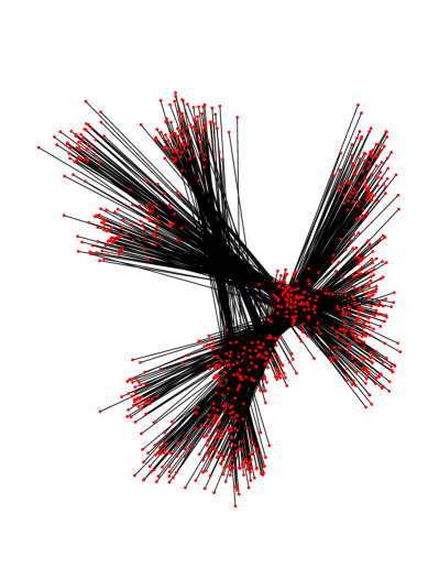
Figure 3: A heuristic MWMP solution for the TSPLIB instance dsj1000 that is within 0.19% of the optimum.

In the class of examples in Fig. 4 we have $\mbox{FWP}(P)=\mbox{FWP}_{num}(P)=\mbox{FWP}_{com}(P)=4M+4$, $\mbox{MWMP}(P)>4M$ and $\mbox{MWMP}_{com}(P)=\mbox{MWMP}_{num}(P)=(2M+4)\sqrt{3}$. So a relative error of about 15% is indeed possible, because the ratio between optimal and heuristic matching may get arbitrarily close to $2/\sqrt{3}$. As we will see further down, this scenario is highly unlikely and the actual error is much smaller for most instances.

Figure 4: A class of examples for which CROSS is 15% away from the optimum.

Furthermore, it is not hard to see that CROSS is optimal if the points are in convex position:

Theorem 1

If the point set $P$ is in convex position, then algorithm CROSS determines the unique optimum.

For a proof, observe that any pair of matching edges in $\mbox{MWMP}(P)$ must be crossing, otherwise we could get an improvement by performing a 2-exchange. So $\mbox{MWMP}(P)=\mbox{MWMP}_{num}(P)$.

2.2 Improving the Upper Bound

When using the value $\mbox{FWP}(P)$ as an upper bound for $\mbox{MWMP}(P)$, we compare the matching edges with pairs of rays, with equality being reached if the angle enclosed between rays is $\pi$, i.e., for points that are on opposite sides of the center point $c$. However, it may well be the case that there is no point opposite to a point $p_{i}$. In that case, we have an upper bound on $\max_{j}\varphi_{ij}$, and we can lower the upper bound $\mbox{FWP}(P)$. See Fig. 5: the distance $d(c,p_{i})$ is replaced by $d(c,p_{i})-\frac{\min_{j\neq i}(d(c,p_{i})+d(c,p_{j})-d(p_{i},p_{j})}{2}$.

Figure 5: Improving the upper bound.

Moreover, we can optimize over the possible location of point $c$. This lowers the value of the upper bound $\mbox{FWP}(P)$, yielding the improved upper bound $\mbox{FWP}^{\prime}(P)$:

$$\mbox{FWP}^{\prime}(P)=\min_{c\in{I\!\!R}^{2}}\sum_{p_{i}\in P}d(c,p_{i})-\frac{\min_{j\neq i}(d(c,p_{i})+d(c,p_{j})-d(p_{i},p_{j})}{2}.$$

This results in a notable improvement, especially for clustered instances. However, computing this modified upper bound $\mbox{FWP}^{\prime}(P)$ is more complicated. (We have used local optimization methods.) Therefore, this approach is only useful for mid-sized instances, and when there is sufficient time.

2.3 An Integrality Result

A standard approach in combinatorial optimization is to model a problem as an integer program, then solve the linear programming relaxation. As it turns out, this works particularly well for the MWMP Tamir and Mitchell (1998):

Theorem 2

Let $x$ be a set of nonnegative edge weights that is optimal for the standard linear programming relaxation of the MWMP, where all vertices are required to be incident to a total edge weight of 1. Then the weight of $x$ is equal to an optimal integer solution of the MWMP.

The proof assumes the existence of two fractional odd cycles, then establishes the existence of an improving 2-exchange by a combination of parity arguments.

Theorem 2 allows us to compute the exact optimum by solving a linear program. For the MWMP, this amounts to solving a network flow problem, which can be done by using a network simplex method. (See Ahuja et al. (1993) for details.)

2.4 Computational Experiments

Table 1 summarizes some of our results for the MWMP for three classes of instances, described below. It shows a comparison of the FWP upper bound with different Matchings: In the first column we list the instance names, in the second column we report the results of the CROSS heuristic for computing a matching. (In all error rates reported, the denominator is the smaller, heuristic value, e.g., we consider $\frac{\mbox{FWP}-\mbox{CROSS}}{\mbox{CROSS}}$ in this column.) The third column shows the corresponding computing times on a Pentium II 500Mhz (using C code with compiler gcc -O3 under Linux 2.2). The fourth column gives the result of combining the CROSS matching with one hour of local search by chained Lin-Kernighan Rohe (1997). The last column compares the optimum computed by a network simplex using Theorem 2 with the upper bound (for $n<10,000$). For the random instances, the average performance over ten different instances is shown.

Instance	CROSS	time	CROSS +	CROSS
	vs. FWP		1h Lin-Ker	vs. OPT
dsj1000	1.22%	0.05 s	1.07%	0.19%
nrw1378	0.05%	0.05 s	0.04%	0.01%
fnl4460	0.34%	0.13 s	0.29%	0.05%
usa13508	0.21%	0.64 s	0.19%	-
brd14050	0.67%	0.59 s	0.61%	-
d18512	0.14%	0.79 s	0.13%	-
pla85900	0.03%	3.87 s	0.03%	-
1000	0.03%	0.05 s	0.02%	0.02%
3000	0.01%	0.14 s	0.01%	0.00%
10000	0.00%	0.46 s	0.00%	-
30000	0.00%	1.45 s	0.00%	-
100000	0.00%	5.01 s	0.00%	-
300000	0.00%	15.60 s	0.00%	-
1000000	0.00%	53.90 s	0.00%	-
3000000	0.00%	159.00 s	0.00%	-
1000c	2.90%	0.05 s	2.82%	0.11 %
3000c	1.68%	0.15 s	1.59%	0.26 %
10000c	3.27%	0.49 s	3.24%	-
30000c	1.63%	1.69 s	1.61%	-
100000c	2.53%	5.51 s	2.52%	-
300000c	1.05%	17.51 s	1.05%	-

Table 1: Maximum matching results for TSPLIB (top), uniform random (center), and clustered random instances (bottom)

The first type of instances are taken from the well-known TSPLIB benchmark library Reinelt (1991). (For odd cardinality TSPLIB instances, we followed the custom of dropping the last point from the list.) Clearly, the relative error decreases with increasing $n$.

The second type was constructed by choosing $n$ points in a unit square uniformly at random. The reader will note that for this distribution, the relative error rapidly converges to zero. This is to be expected: for uniform distribution, the expected angle $\angle(p_{i},c,p_{i+n/2})$ becomes arbitrarily close to $\pi$. In more explicit terms: Both the value $\mbox{FWP}(P)/n$ and $\mbox{MWMP}(P)/n$ for a set of $n$ random points in a unit square tend to the limit
$\int_{-1/2}^{1/2}\int_{-1/2}^{1/2}\sqrt{x^{2}+y^{2}}dxdy\approx 0.3826$.

The third type uses $n$ points that are chosen by selecting random points from a relatively small expected number $k$ of “cluster” areas. Within each cluster, points are located with uniform polar coordinates (with some adjustment for clusters near the boundary) with a circle of radius 0.05 around a central point, which is chosen uniformly at random from the unit square. This type of instances is designed to make our heuristic look bad; for this reason, we have shown the results for $k=5$. See Fig. 6 for a typical example with $n=10,000$.

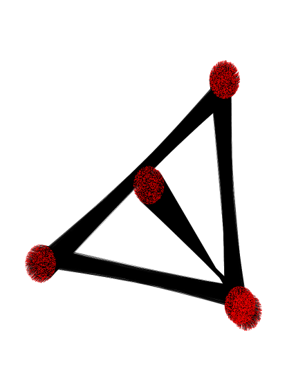
Figure 6: A typical cluster example with its matching.

It is not hard to see that these cluster instances behave very similar to fractional solutions of the standard LP relaxation for instances with $|V^{\prime}|=k$ points, where the objective is to find a set of non-negative edge weights of maximum total value, such that the total weight of the set $\delta(v)$ of edges incident to a vertex $v\in V^{\prime}$ has total weight of 1:

$$\mbox{ max }c^{t}x$$

with

$$\begin{array}[]{rcrr}\sum_{e\in\delta(v)}x_{e}&=&1&\forall v\in V^{\prime}\\ x_{e}&\geq&0.\end{array}$$

Moreover, for increasing $k$, we approach a uniform random distribution over the whole unit square, meaning that the performance is expected to get better. But even for small $k$, it should be noted that for small instances, the remaining error estimate is almost entirely due to limited performance of the upper bound. The good quality of our fast heuristic for large problems is illustrated by the fact that one hour of local search by Lin-Kernighan fails to provide any significant improvement.

3 The Maximum TSP

As we noted in the introduction, the geometric MTSP displays some peculiar properties when distances are measured according to some polyhedral norm. In fact, it was shown by Fekete (1999) that for the case of Manhattan distances in the plane, the MTSP can be solved in linear time. (The algorithm is based in part on the observation that for planar Manhattan distances, $\mbox{FWP}(P)=\mbox{MWMP}(P)$.) On the other hand, it was shown in the same paper that for Euclidean distances in ${I\!\!R}^{3}$ or on the surface of a sphere, the MTSP is NP-hard. The MTSP has also been conjectured to be NP-hard for the case of Euclidean distances in ${I\!\!R}^{2}$. For further details, see the paper Barvinok et al. (2002).

3.1 A Worst-Case Estimate

Clearly, there are some observations for the MWMP that can be applied to the MTSP. In particular, we note that $\mbox{MTSP}(P)\leq 2\cdot\mbox{MWMP}(P)\leq 2\cdot\mbox{FWP}(P)$. On the other hand, the inequality $\mbox{FWP}(P)\leq\mbox{MWMP}(P)\cdot 2/\sqrt{3}$ does not imply that $2\cdot\mbox{FWP}(P)\leq\mbox{MTSP}(P)\cdot 2/\sqrt{3}$. Figure  7 shows a set of points $P$ for which $2\cdot\mbox{FWP}(P)=\mbox{MTSP}(P)\cdot 4/(2+\sqrt{2})\approx 1.17\cdot\mbox{MTSP}(P)$.

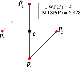
Figure 7: An example for which the ratio between $2\cdot\mbox{FWP}(P)$ and $\mbox{MTSP}(P)$ is greater than $2/\sqrt{3}\approx 1.15$.

However, we can argue that asymptotically, the worst-case ratio $2\cdot\mbox{FWP}(P)/\mbox{MTSP}(P)$ is $2/\sqrt{3}$, which is also the worst case ratio for $\mbox{FWP}(P)/\mbox{MWMP}(P)$.

Theorem 3

For $n\!\rightarrow\!\infty$, the worst-case ratio of $2\cdot\mbox{FWP}(P)/\mbox{MTSP}(P)$ tends to $2/\sqrt{3}$.

Proof 3.4.

Consider a set of $n$ points where $n$ is a multiple of 3. Suppose $n/3$ points are at position (-2,0), $n/3$ points at location $(1,\sqrt{3})$ and $n/3$ points at location $(1,-\sqrt{3})$. We have $2\mbox{FWP}(P)/\mbox{MTSP}(P)=2/\sqrt{3}$. We show that this bound is asymptotically tight.

The proof of the $2/\sqrt{3}$ bound for the MWMP in Fekete and Meijer (2000) establishes that any planar point set can be subdivided by six sectors of $\pi/3$ around one center point, such that opposite sectors have the same number of points. Connecting points from opposite sectors gives the matching $\mbox{MWMP}_{com}$, establishing a lower bound of $2\pi/3$ for the angle between the corresponding rays. This means that we can simply choose three subtours, one for each pair of opposite sectors, as shown in Figure 8(a). For the total length SUB$(P)$ of these subtours, $S_{1}$, $S_{2}$, $S_{3}$, we get $2\mbox{FWP}(P)/\mbox{SUB}(P)\leq 2/\sqrt{3}$. In order to merge these subtours, let $e_{1}=(v_{1},w_{1})$ and $e_{2}=(v_{2},w_{2})$ be two shortest edges in $S=S_{1}\cup S_{2}\cup S_{3}$. Let $e_{3}=(v_{3},w_{3})\neq e_{2}$ be any edge in $S$ not in the same subtour as $e_{1}$. Then we can perform a 2-exchange with the two edges $e_{1}$ and $e_{3}$, i.e., replace $e_{1}$ and $e_{3}$ by $e_{5}=(v_{1},w_{3})$ and $e_{6}=(v_{3},w_{1})$, as shown in Figure 8(b). This merges the subtours containing $e_{1}$ and $e_{3}$ into a single subtour. Using $e_{2}$ for a second 2-exchange, we obtain a tour. By triangle inequality, we have $d(v_{3},w_{3})\leq d(v_{3},w_{1})+d(w_{1},v_{1})+d(v_{1},w_{3})$, i.e., the length of $e_{3}$ is bounded by the combined length of $e_{1}$, $e_{5}$, $e_{6}$. Thus, the first 2-exchange reduces the total length by at most $2d(v_{1},w_{1})$. Similarly, the second exchange reduces the total length by at most $2d(v_{2},w_{2})$. Therefore, the resulting tour has length at least $(n-4)\mbox{SUB}(P)/n$, and we conclude $2\mbox{FWP}(P)/\mbox{MTSP}(P)\leq 2n/\sqrt{3}(n-4)$. As $n$ grows, this tends to $2/\sqrt{3}$, as claimed.

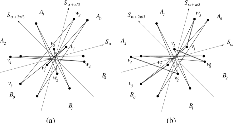
Figure 8: (a) Three subtours that connect only points from opposite sectors, guaranteeing $2\mbox{FWP}(P)/\mbox{SUB}(P)\leq 2/\sqrt{3}$. (b) Merging the subtours by using two short edges.

3.2 A Heuristic Solution

It is easy to determine a maximum tour if we are dealing with an odd number of points in convex position: Each point $p_{i}$ gets connected to its two “cyclic furthest neighbors” $p_{i+{\lfloor n/2\rfloor}}$ and $p_{i+{\lceil n/2\rceil}}$. However, the structure of an optimal tour is less clear for a point set of even cardinality, and therefore it is not obvious what permutations should be considered for an analogue to the matching heuristic CROSS. For this we consider the local modification called 2-exchanges. Consider a set $T$ of directed edges such that each point $p_{i}$ has exactly one incoming and one outgoing edge. Notice that $T$ is a collection of cycles. In a 2-exchange in $T$ we replace edges $(p_{i},p_{k})$ and $(p_{j},p_{l})$ by edges $(p_{i},p_{j})$ and $(p_{l},p_{k})$. We then redirect the edges so that $T$ forms a collection of cycles.

Algorithm CROSS’: Heuristic solution for MTSP Input: A set of points $P\in{I\!\!R}^{2}$. Output: A tour of $P$. 1. Using a numerical method, find a point $c$ that approximately minimizes the convex function $\min_{c\in{I\!\!R}^{2}}\sum_{p_{i}\in P}d(c,p_{i})$. 2. Sort the set $P$ by angular order around $c$. Assume the resulting order is $p_{1},\ldots,p_{n}$. 3. If $n$ is odd, then for $i=1,\ldots,n$, connect point $p_{i}$ with point $p_{i+(n-1)/2}$. Return the resulting tour and quit the algorithm. 4. If $n$ is even, then for $i=1,\ldots,n$, connect point $p_{i}$ with point $p_{i+n/2-1}$. Compute the resulting total length $L$. 5. Compute $D=\max_{i=1}^{n}[d(p_{i},p_{i+n/2})+d(p_{i+1},p_{i+1+n/2})$ $-d(p_{i},p_{i+n/2+1})-d(p_{i+1},p_{i+n/2})]$. 6. Execute the 2-exchange that increases the tour by $D$. Return this tour.

Figure 9: The heuristic CROSS’

Theorem 3.5.

If the point set $P$ is in convex position with $n$ even, then there are at most $n/2$ tours that are locally optimal with respect to 2-exchanges, and we can determine the best in linear time.

Proof 3.6.

Assume that $P=\{p_{1},p_{2},\cdots,p_{n}\}$ is given is angular order. Assume arithmetic in the indices is done $\bmod~{}n$. We claim that any tour that is locally optimal with respect to 2-exchanges must look like the one in Fig. 10. It consists of two diagonals $(p_{i},p_{i+n/2})$ and $(p_{i+1},p_{i+1+n/2})$ (in the example, these are the edges $(5,11)$ and $(6,0)$), while all other edges are near-diagonals, i.e., edges of the form $(p_{j},p_{j+n/2-1})$.

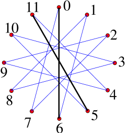
Figure 10: A locally optimal MTSP tour.

Consider a set $T$ of directed edges such that each point in $P$ has exactly one incoming and one outgoing edge, i.e., a collection of cycles. The length of $T$ is the sum of the lengths of the edges in $T$. Let $e_{i}=(p_{i},p_{k})$ and $e_{j}=(p_{j},p_{l})$ be two edges in $T$. Consider the quadrilateral formed by the points $p_{i},p_{j},p_{k}$ and $p_{l}$, as shown in Figure 11.

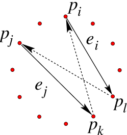
Figure 11: Two parallel edges $e_{i}$ and $e_{j}$.

We say that $e_{i}$ and $e_{j}$ areparallel if they do not cross, if they lie in the same cycle of $T$ and if one of the edges is directed in a clockwise direction around the quadrilateral and the other edge is directed in a counter-clockwise direction around the quadrilateral. We say that $e_{i}$ and $e_{j}$ are antiparallel if they do not cross and are not parallel.

We will show that if $T$ has a maximal length with respect to 2-exchanges, then $T$ is a tour. Consider 2-exchanges that increase the length of $T$. It is an easy consequence of triangle inequality that antiparallel edges such as $e_{0}=(0,4)$ and $e_{1}=(5,10)$ in Fig. 12(a) allow a crossing 2-exchange that increases the overall length of $T$: This follows from the fact that the length of two crossing diagonals in a quadrilateral must exceed the length of any two opposite edges of that quadrilateral. Crucial for the feasibility of this exchange is the orientation of the directed edges; the exchange is possible if the edges are antiparallel. In the following, we will focus on identifying antiparallel edge pairs.

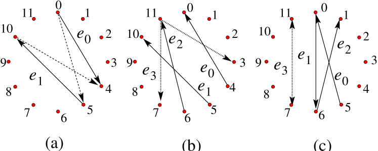
Figure 12: Discussing locally optimal tours.

We first show that all edges in a locally optimal collection $T$ must be diagonals or near-diagonals. Consider an edge $e_{0}=(p_{i},p_{j})$ with $0<j-i\leq n/2-2$. Then there are at most $n/2-3$ points in the subset $P_{1}=[p_{i+1},\ldots,p_{j-1}]$, and at least $n/2+1$ points in the subset $P_{2}=[p_{j+1},\ldots,p_{i-1}]$. This implies that there must be at least two edges (say, $e_{1}$ and $e_{2}$) within the subset $P_{2}$. If either of them is antiparallel to $e_{0}$, we are done, so assume that both of them are parallel to $e_{0}$. Without loss of generality assume that the head of $e_{2}$ lies “between” the head of $e_{1}$ and the head $p_{j}$ of $e_{0}$, as shown in Fig. 12(b). Then the edge $e_{3}$ that is the successor of $e_{2}$ in $T$ is either antiparallel with $e_{1}$, or with $e_{0}$.

Next consider a collection $T$ consisting only of diagonals and near-diagonals. Since there is only one 2-factor consisting of nothing but near-diagonals, assume without loss of generality that there is at least one diagonal, say $e_{1}=(p_{0},p_{n/2})$. Suppose the successor $e_{2}$ of $e_{1}$ and the predecessor $e_{0}$ of $e_{1}$ lie on the same side of $e_{1}$, as shown in Fig. 12(c). Then there must be an edge $e_{3}$ within the set of points on the other side of $e_{0}$. Edge $e_{3}$ does not cross $e_{0}$ nor $e_{1}$; so either it is antiparallel to $e_{0}$ or to $e_{1}$, and $T$ is not optimal.

Therefore the edges $e_{0}$ and $e_{2}$ lie on different sides of the diagonal $e_{1}$. This means that once the diagonal $e_{1}$ has been chosen, the rest of the tour is determined: each following edge must be a near-diagonal that crosses $e_{1}$. The resulting $T$ must look as in Fig. 10, concluding the proof.

This motivates a heuristic analogous to the one for the MWMP. For simplicity, we call it CROSS’. Assume that in Algorithm CROSS’ of Fig. 9, we use the center of $\mbox{FWP}_{com}(P)$ as the point $c$ in step 1. Let $\mbox{CROSS}^{\prime}(P)$ denote the value of the tour found by algorithm CROSS’. From the proof of Theorem 3 we know that for $n\!\rightarrow\!\infty$, $2\cdot\mbox{FWP}_{com}(P)\leq\mbox{CROSS}^{\prime}(P)\cdot 2/\sqrt{(}3)$. This implies $\mbox{MTSP}(P)~{}\leq~{}2\cdot\mbox{FWP}(P)~{}\leq~{}\mbox{CROSS}^{\prime}(P)\cdot 2/\sqrt{(}3)$. Fig. 13 shows that this bound can be achieved.

Figure 13: A class of examples for which the ratio between $2\cdot\mbox{FWP}(P)$ and the heuristic solution computed by CROSS’ is arbitrarily close to $2/\sqrt{3}$. Moreover, the ratio of $\mbox{MTSP}(P)$ and CROSS’ is also $2/\sqrt{3}$. The circle has unit radius, $X$ is large. Shown is the heuristic tour; an optimal solution has no connections between the “far away” clusters of size $s$.

If we use the center of $\mbox{FWP}_{num}(P)$ rather than the center of $\mbox{FWP}_{com}(P)$ we expect a better performance for algorithm CROSS’. The following lemma shows that CROSS’ is optimal for points in convex position. The computational results in the next section show that CROSS’ performs very well.

Theorem 3.7.

If the point set $P$ is in convex position, then algorithm CROSS’ determines the optimum.

Proof 3.8.

Let $n$ denote the number of points in $P$. If $n$ is even, the result follows from Theorem 3.5. For odd values of $n$, a proof similar to the one of Theorem 3.5 can be constructed to show that an optimal tour consists only of near-diagonals. Such a tour is unique and will be found by the algorithm CROSS’.

3.3 No Integrality

As the example in Fig. 14 shows, there may be fractional optima for the subtour relaxation of the MTSP:

$$\mbox{ max }c^{t}x$$

with

$$\begin{array}[]{rcrr}\sum_{e\in\delta(v)}x_{e}&=&2&\forall v\in V\\ \sum_{e\in\delta(S)}x_{e}&\geq&2&\ \ \forall\emptyset\neq S\subset V\\ x_{e}&\geq&0.\end{array}$$

The fractional solution consists of all diagonals (with weight 1) and all near-diagonals (with weight 1/2). It is easy to check that this solution is indeed a vertex of the subtour polytope, and that it beats any integral solution. (See Boyd and Pulleyblank (1991) on this matter.) This implies that there is no simple analogue to Theorem 2 for the MWMP, and we do not have a polynomial method that can be used for checking the optimal solution for small instances.

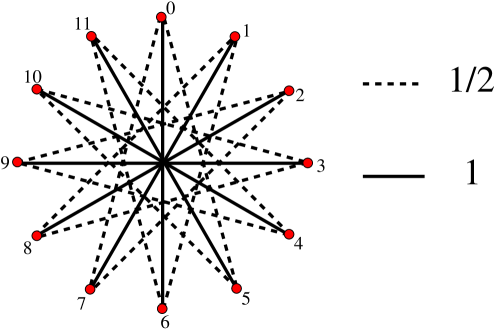
Figure 14: A fractional optimum for the subtour relaxation of the MTSP.

3.4 Computational Results

The results are of similar quality as for the MWMP. See Table 2. Here we only give the results for the seven most interesting TSPLIB instances. Since we do not have a comparison with the optimum for small instances, we give a comparison with the upper bound 2MAT, denoting twice the optimal solution for the MWMP. As before, this was computed by a network simplex method, exploiting the integrality result for planar MWMP. The results show that here, too, most of the remaining gap lies on the side of the upper bound.

Instance	CROSS’	time	CROSS’ +	CROSS’
	vs. FWP		1h Lin-Ker	vs. 2MAT
dsj1000	1.36%	0.05 s	1.10%	0.329%
nrw1379	0.23%	0.01 s	0.20%	0.194%
fnl4461	0.34%	0.12 s	0.31%	0.053%
usa13509	0.21%	0.63 s	0.19%	-
brd14051	0.67%	0.46 s	0.64%	-
d18512	0.15%	0.79 s	0.14%	-
pla85900	0.03%	3.87 s	0.03%	-
1000	0.04%	0.06 s	0.02%	0.02%
3000	0.02%	0.16 s	0.01%	0.00%
10000	0.01%	0.48 s	0.00%	-
30000	0.00%	1.47 s	0.00%	-
100000	0.00%	5.05 s	0.00%	-
300000	0.00%	15.60 s	0.00%	-
1000000	0.00%	54.00 s	0.00%	-
3000000	0.00%	160.00 s	0.00%	-
1000c	2.99%	0.05 s	2.87%	0.11 %
3000c	1.71%	0.15 s	1.61%	0.26 %
10000c	3.28%	0.49 s	3.25%	-
30000c	1.63%	1.69 s	1.61%	-
100000c	2.53%	5.51 s	2.52%	-
300000c	1.05%	17.80 s	1.05%	-

Table 2: Maximum TSP results for TSPLIB (top), uniform random (center), and clustered random instances (bottom)

Table 3 shows an additional comparison for TSPLIB instances of moderate size. Shown are (1) the tour length found by our fastest heuristic; (2) the relative gap between this tour length and the fast upper bound; (3) the tour length found with additional Lin-Kernighan; (4) “optimal” values computed by using the Concorde code for solving Minimum TSPs; (5) and (6) the two versions of our upper bound; (7) the maximum version of the well-known Held-Karp bound. In order to apply Concorde, we have to transform the MTSP into a Minimum TSP instance with integer edge lengths. As the distances for geometric instances are not integers, it has become customary to transform distances into integers by rounding to the nearest integer. When dealing with truly geometric instances, this rounding introduces a certain amount of inaccuracy on the resulting optimal value: Table 3 shows two results for the value OPT: The smaller one is the true value of the “optimal” tour that was computed by Concorde for the rounded distances, the second one is the value obtained by re-transforming the rounded objective value. As can be seen from the table, even the tours constructed by our near-linear heuristic can beat the “optimal” value, and the improved heuristic value almost always does. This shows that our heuristic approach yields results within a widely accepted margin of error; furthermore, it illustrates that thoughtless application of a time-consuming “exact” methods may yield a worse performance than using a good and fast heuristic. Of course it is possible to overcome this problem by using sufficiently increased accuracy; however, it is one of the long outstanding open problems on the Euclidean TSP whether there is a sufficient accuracy that is polynomial in terms of $n$. This amounts to deciding whether the Euclidean TSP is in NP. See Johnson and Papadimitriou (1985).

The Held-Karp bound (which is usually quite good for Min TSP instances) can also be computed as part of the Concorde package. However, it is relatively time-consuming when used in its standard form: We allowed for 20 minutes for instances with $n\approx 100$, and considerably more for larger instances. Clearly, this bound is not very tight for geometric MTSP instances, as it is is outperformed by our much faster geometric heuristics.

Instance	CROSS’	CROSS’	CROSS’	OPT	FWP’	FWP	HK
		vs. FWP	+ Lin-Ker	via Concorde			bound
eil101	4966	0.15%	4966	[4958, 4980]	4971	4973	4998
bier127	840441	0.16%	840810	[840811, 840815]	841397	841768	846486
ch150	78545	0.12%	78552	[78542, 78571]	78614	78638	78610
gil262	39169	0.05%	39170	[39152, 39229]	39184	39188	39379
a280	50635	0.13%	50638	[50620, 50702]	50694	50699	51112
lin318	860248	0.09%	860464	[860452, 860512]	860935	861050	867060
rd400	311642	0.05%	311648	[311624, 311732]	311767	311767	314570
fl417	779194	0.18%	779236	[779210, 779331]	780230	780624	800402
rat783	264482	0.00%	264482	[264431, 264700]	264492	264495	274674
d1291	2498230	0.06%	2498464	[2498446, 2498881]	2499627	2499657	2615248

Table 3: Maximum TSP results for small TSPLIB instances: Comparing CROSS’ and FWP with other bounds and solutions.

References

- Ahuja et al. (1993) \bibscAhuja, R., Magnanti, T., and Orlin, J. \bibyear1993. \bibemphNetwork flows. Theory, algorithms and applications. Prentice-Hall, New-York.
- Applegate et al. (1998) \bibscApplegate, D., Bixby, R., Chvátal, V., and Cook, W. \bibyear1998. On the solution of traveling salesman problems. \bibemphicDocumenta Mathematica \bibemphExtra Volume Proceedings ICM III (1998), 645–656.
- Arora (1998) \bibscArora, S. \bibyear1998. Polynomial time approximation schemes for Euclidean traveling salesman and other geometric problems. \bibemphicJournal of the ACM \bibemph45, 5, 753–782.
- Bajaj (1988) \bibscBajaj, C. \bibyear1988. The algebraic degree of geometric optimization problems. \bibemphicDiscrete Comput. Geom. \bibemph3, 177–191.
- Barvinok et al. (2002) \bibscBarvinok, A. I., Fekete, S. P., Johnson, D. S., Tamir, A., Woeginger, G. J., and Woodroofe, R. \bibyear2002. The geometric maximum traveling salesman problem. \bibemphichttp://arxiv.org/abs/cs.DS/0204024.
- Barvinok et al. (1998) \bibscBarvinok, A. I., Johnson, D. S., Woeginger, G. J., and Woodroofe, R. \bibyear1998. The maximum traveling salesman problem under polyhedral norms. In \bibemphicProceedings of the 6th International Conference on Integer Programming and Combinatorial Optimization (IPCO), Volume 1412 of \bibemphLecture Notes in Computer Science (1998), pp. 195–201. Springer-Verlag.
- Boyd and Pulleyblank (1991) \bibscBoyd, S. C. and Pulleyblank, W. R. \bibyear1990/1991. Optimizing over the subtour polytope of the travelling salesman problem. \bibemphicMathematical Programming \bibemph49(2), 163–187.
- Cook and Rohe (1999) \bibscCook, W. and Rohe, A. \bibyear1999. Computing minimum-weight perfect matchings. \bibemphicINFORMS Journal on Computing \bibemph11, 138–148.
- Edmonds (1965a) \bibscEdmonds, J. \bibyear1965a. Maximum matching and a polyhedron with 0,1 vertices. \bibemphicJ. Res. Nat. Bur. Standards (B) \bibemph69, 125–130.
- Edmonds (1965b) \bibscEdmonds, J. \bibyear1965b. Paths, trees, and flowers. \bibemphicCanad. J. Math. \bibemph17, 449–467.
- Fekete (1999) \bibscFekete. \bibyear1999. Simplicity and hardness of the maximum traveling salesman problem under geometric distances. In \bibemphicProceedings of SODA 1999: ACM-SIAM Symposium on Discrete Algorithms (1999), pp. 337–345.
- Fekete and Meijer (2000) \bibscFekete, S. P. and Meijer, H. \bibyear2000. On minimum stars, minimum Steiner stars, and maximum matchings. \bibemphicDiscrete and Computational Geometry \bibemph23, 340a, 389–407.
- Fekete et al. (2001) \bibscFekete, S. P., Meijer, H., Rohe, A., and Tietze, W. \bibyear2001. Solving a “hard” problem to approximate an “easy” one: Heuristics for maximum matchings and maximum traveling salesman problems. In \bibemphicProceedings of the Third International Workshop on Algorithm Engineering and Experiments (ALENEX), Volume 2153 of \bibemphLecture Notes in Computer Science (2001), pp. 1–16. Springer-Verlag.
- Gabow (1990) \bibscGabow, H. \bibyear1990. Data structures for weighted matching and nearest common ancestors with linking. In \bibemphicProceedings of the 1st Annual ACM–SIAM Symposium on Discrete Algorithms (1990), pp. 434–443. ACM Press.
- Held and Karp (1971) \bibscHeld, M. and Karp, R. M. \bibyear1971. The traveling salesman problem and minimum spanning trees: Part ii. \bibemphicMathematical Programming \bibemph1, 6–25.
- Johnson and Papadimitriou (1985) \bibscJohnson, D. S. and Papadimitriou, C. H. \bibyear1985. Computational complexity. In \bibscE. L. Lawler, J. K. Lenstra, A. H. G. R. Kan, and D. B. Shmoys Eds., \bibemphicThe traveling salesman problem, Chapter 3, pp. 37–85. Chichester: Wiley.
- Kuhn (1973) \bibscKuhn, H. W. \bibyear1973. A note on Fermat’s problem. \bibemphicMath. Programming \bibemph4, 98–107.
- Mehlhorn and Schäfer (2000) \bibscMehlhorn, K. and Schäfer, G. \bibyear2000. Implementation of o(nm log n) weighted matchings in general graphs: The power of data structures. In \bibemphicProceedings of the 3rd Workshop on Algorithm Engineering, Volume 1982 of \bibemphLecture Notes in Computer Science (2000), pp. 23–38. Springer-Verlag.
- Mitchell (1999) \bibscMitchell, J. S. B. \bibyear1999. Guillotine subdivisions approximate polygonal subdivisions: A simple polynomial-time approximation scheme for geometric TSP, -MST, and related problems. \bibemphicSIAM Journal on Computing \bibemph28, 4, 1298–1309.
- Reinelt (1991) \bibscReinelt, G. \bibyear1991. TSPLIB: A traveling salesman problem library. \bibemphicORSA Journal on Computing, http://www.iwr.uni-heidelberg.de/groups/comopt/software/TSPLIB95/ \bibemph3, 376–384.
- Richter-Gebert and Kortenkamp (1999) \bibscRichter-Gebert, J. and Kortenkamp, U. \bibyear1999. \bibemphThe Interactive Geometry Software Cinderella. Springer-Verlag, Heidelberg.
- Rohe (1997) \bibscRohe, A. \bibyear1997. Parallele Heuristiken für sehr große Traveling Salesman Probleme. Master’s thesis, Universität Bonn.
- Tamir and Mitchell (1998) \bibscTamir, A. and Mitchell, J. S. B. \bibyear1998. A maximum -matching problem arising from median location models with applications to the roommates problem. \bibemphicMath. Programming \bibemph80, 171–194.
- Vaidya (1989) \bibscVaidya, P. M. \bibyear1989. Geometry helps in matching. \bibemphicSIAM J. Comput. \bibemph18, 6, 1201–1225.
- Valenzuela and Jones (1997) \bibscValenzuela, C. L. and Jones, A. J. \bibyear1997. Estimating the Held-Karp lower bound for the geometric TSP. \bibemphicEuropean Journal of Operational Research \bibemph102, 157–175.
- Varadarajan (1998) \bibscVaradarajan, K. R. \bibyear1998. A divide-and-conquer algorithm for min-cost perfect matching in the plane. In \bibemphicIEEE Symposium on Foundations of Computer Science (1998), pp. 320–331.
- Weiszfeld (1937) \bibscWeiszfeld, E. \bibyear1937. Sur le point pour lequel la somme des distances de n points donnés est minimum. \bibemphicTôhoku Math. J. \bibemph43, 355–386.