Qualitative study of a robot arm as a hamiltonian system

Abstract

A double pendulum subject to external torques is used as a model to study the stability of a planar manipulator with two links and two rotational driven joints. The hamiltonian equations of motion and the fixed points (stationary solutions) in phase space are determined. Under suitable conditions, the presence of constant torques does not change the number of fixed points, and preserves the topology of orbits in their linear neighborhoods; two equivalent invariant manifolds are observed, each corresponding to a saddle-center fixed point.

I Introduction

The problem of the stability of motion and equilibrium of manipulators is essential to their applicability in industry. In this work, we analyze the stability of one class of such manipulators, namely, planar manipulators with two links and two rotational driven joints (see Fig.1), modelled by a double pendulum subject to two constant external torques $T_{1}$ and $T_{2}$(see Fig.2). Each pendulum has lenght $L$ and has a particle of mass $m$ attached to its end.

Figure 1: Simplified diagram of a planar manipulator with two links.

Figure 2: Double pendulum model for the planar manipulator in Fig.1. The pendulum is subject to the external torques $T1$ and $T2$ at points $A$ and $B$, respectively.

For any given configuration $(\theta_{1},\theta_{2})$ where $0\leq\theta_{1}\leq 2\pi$ and $0\leq\theta_{1}\leq 2\pi$, and conjugate momenta $p_{1}=p_{2}=0$, the torques $T_{1}$ and $T_{2}$ can be adjusted so that this configuration become stationary. In this work we will study the dynamics of this system in the linear neighborhod of stationary configurations under constant external torques.

As indicated in Fig.2, the model consists of a combination of two simple pendula with equal length $L$, where the two drivers are represented by external torques $T_{1}$ and $T_{2}$ applied at points $A$ and $B$, respectively. For the sake of simplicity, we shall consider the mass $m$ of the object held by the end-effector $C$ as being equal to the mass of the driver in $B$.

We apply qualitative analysis techniquesahmed ; hagedorn ; meirovitch suitable to non-linear systems, using the hamiltonian formalism.

II Dynamics of the model

The system depicted in Fig.2 can be represented by the following hamiltonian function with two degrees of freedom:

$$H = \frac{1}{mL^{2}\left(1+sen^{2}\left({\theta}_{1}-{\theta}_{2}\right)\right)}\left\{\frac{p_{1}^{2}}{2}+p_{2}^{2}-cos\left({\theta}_{1}-{\theta}_{2}\right)p_{1}p_{2}\right\}+$$ (1)

$$-mgL\left(\cos({\theta}_{1})+2\cos({\theta}_{2})\right)-{\theta}_{1}T_{1}(t)-{\theta}_{2}T_{2}(t),$$

where $g$ is the acceleration of gravity and $(p_{1},p_{2})$ are the conjugate momenta to the angular variables $({\theta}_{1},{\theta}_{2})$, respectively. The functions $T_{1}(t)$ and $T_{2}(t)$ stand for arbitrary external torques on the system. The hamiltonian equations of motion yield the non-integrable, non-linear dynamical system

$$\dot{{\theta}_{1}}=\frac{\partial H}{\partial{p}_{1}} = \frac{p_{1}-\cos({\theta}_{1}-{\theta}_{2})p_{2}}{mL^{2}\left(1+\sin^{2}({\theta}_{1}-{\theta}_{2})\right)}$$ (2)

$$\dot{p_{1}}=-\frac{\partial H}{\partial{\theta}_{1}} = \frac{\left(p_{1}^{2}+2p_{2}^{2}-2\cos({\theta}_{1}-{\theta}_{2})p_{1}p_{2}\right)\cos(\theta_{1}-\theta_{2})\sin({\theta}_{1}-{\theta}_{2})}{mL^{2}\left(1+\sin^{2}({\theta}_{1}-{\theta}_{2})\right)^{2}}+$$ (3)

$$-\frac{\sin({\theta}_{1}-{\theta}_{2})p_{1}p_{2}}{mL^{2}(1+\sin^{2}({\theta}_{1}-{\theta}_{2}))}-2mgL\sin({\theta}_{1})+T_{1}(t)$$

$$\dot{{\theta}_{2}}=\frac{\partial H}{\partial{p}_{2}} = \frac{2p_{2}-\cos({\theta}_{1}-{\theta}_{2})p_{1}}{mL^{2}\left(1+\sin^{2}({\theta}_{1}-{\theta}_{2})\right)}$$ (4)

$$\dot{p_{2}}=-\frac{\partial H}{\partial{\theta}_{2}} = -\frac{\left(p_{1}^{2}+2p_{2}^{2}-2\cos({\theta}_{1}-{\theta}_{2})p_{1}p_{2}\right)\cos({\theta}_{1}-{\theta}_{2})\sin({\theta}_{1}-{\theta}_{2})}{mL^{2}\left(1+\sin^{2}({\theta}_{1}-{\theta}_{2})\right)^{2}}+$$ (5)

$$+\frac{\sin({\theta}_{1}-{\theta}_{2})p_{1}p_{2}}{mL^{2}\left(1+\sin^{2}({\theta}_{1}-{\theta}_{2})\right)}-mgL\sin({\theta}_{2})+T_{2}(t).$$

We will search for fixed points in phase space. At first, we will let $T_{1}=T_{2}=0$ and discuss the case of null external torques; afterwards, we shall treat the case of non-null constant external torques.

III The robot arm with null external torques

Hamilton equations (2) and (5) have four fixed points. Namely,

000),𝒫4=(π0π0).formulae-sequencesubscript𝒫10000formulae-sequencesubscript𝒫200𝜋0formulae-sequencesubscript𝒫3 000subscript𝒫4𝜋0𝜋0{\cal P}_{1}=\left(\begin{tabular}[]{c}0\\ 0\\ 0\\ 0\end{tabular}\right),\ \ {\cal P}_{2}=\left(\begin{tabular}[]{c}0\\ 0\\ $\pi$\\ 0\end{tabular}\right),\ \ {\cal P}_{3}=\left(\begin{tabular}[]{c}$\pi$\\ 0\\ 0\\ 0\end{tabular}\right),\ \ {\cal P}_{4}=\left(\begin{tabular}[]{c}$\pi$\\ 0\\ $\pi$\\ 0\end{tabular}\right).

$${𝒫}_1=\left(\begin{array}{c}\text{0}\\ \text{0}\\ \text{0}\\ \text{0}\end{array}\right),{𝒫}_2=\left(\begin{array}{c}\text{0}\\ \text{0}\\ \pi \\ \text{0}\end{array}\right),{𝒫}_3=(\begin{array}{c}\end{array}$$ππ (6)

where the matrix lines are ordered from top to bottom according to the coordinates $(\theta_{1},p_{1},\theta_{2},p_{2})$, respectively. The total energies associated to each fixed point are

$$E_{1}=-3mgL\mbox{\hskip 14.22636pt , \hskip 14.22636pt}E_{2}=-mgL\mbox{\hskip 14.22636pt , \hskip 14.22636pt}E_{3}=+mgL\mbox{\hskip 14.22636pt , \hskip 14.22636pt}E_{4}=+3mgL.$$ (7)

Upon linearization of the system of Hamilton equations, we obtain

$$\dot{X}_{i}=J_{i}X_{i},$$ (8)

where $i=1,2,3,4$ labels the fixed points. The vector $X_{i}$ has the general form $\tilde{X}_{i}=(\theta_{1},p_{1},\theta_{2},p_{2})$, and the jacobian matrices $J_{i}$ are

$$J_{1}=\left(\begin{array}[]{cccc}0&\frac{1}{mL^{2}}&0&-\frac{1}{mL^{2}}\\ -2mgL&0&0&0\\ 0&-\frac{1}{mL^{2}}&0&\frac{2}{mL^{2}}\\ 0&0&-mgL&0\\ \end{array}\right),$$ (9)

$$J_{2}=\left(\begin{array}[]{cccc}0&\frac{1}{mL^{2}}&0&\frac{1}{mL^{2}}\\ -2mgL&0&0&0\\ 0&\frac{1}{mL^{2}}&0&\frac{2}{mL^{2}}\\ 0&0&mgL&0\\ \end{array}\right),$$ (10)

$$J_{3}=\left(\begin{array}[]{cccc}0&\frac{1}{mL^{2}}&0&\frac{1}{mL^{2}}\\ 2mgL&0&0&0\\ 0&\frac{1}{mL^{2}}&0&\frac{2}{mL^{2}}\\ 0&0&-mgL&0\\ \end{array}\right),$$ (11)

$$J_{4}=\left(\begin{array}[]{cccc}0&\frac{1}{mL^{2}}&0&-\frac{1}{mL^{2}}\\ 2mgL&0&0&0\\ 0&-\frac{1}{mL^{2}}&0&\frac{2}{mL^{2}}\\ 0&0&mgL&0\\ \end{array}\right).$$ (12)

The general solution to the linearized system (8) around a fixed point is a superposition of four independent solutions,

$$X_{i}(t)=\sum_{m=1}^{4}c^{(i)}_{m}e^{\lambda^{(i)}_{n}t}A^{(i)}_{m},$$ (13)

where $A^{(i)}_{m}$ are the eigenvectors associated to the eigenvalues ${\lambda}^{(i)}_{n}$ of $J_{i}$, and the coefficients $c^{(i)}_{n}$ are integration constants that depend on the initial conditions. The eigenvalues associated to the $J_{i}$ matrices are, respectively,

$$J_{1}: \lambda^{(1)}_{1,2}=\pm i\omega_{0}\sqrt{2-\sqrt{2}}\mbox{\hskip 14.22636pt and \hskip 14.22636pt}{\lambda}^{(1)}_{3,4}=\pm i\omega_{0}\sqrt{2+\sqrt{2}}~{};$$ (14)

$$J_{2}: {\lambda}^{(2)}_{1,2}=\pm\omega_{0}\sqrt[4]{2}\mbox{\hskip 14.22636pt and \hskip 14.22636pt}{\lambda}^{(2)}_{3,4}=\pm i\ \omega_{0}\sqrt[4]{2}~{};$$ (15)

$$J_{3}: {\lambda}^{(3)}_{1,2}=\pm\omega_{0}\sqrt[4]{2}\mbox{\hskip 14.22636pt and \hskip 14.22636pt}{\lambda}^{(3)}_{3,4}=\pm i\ \omega_{0}\sqrt[4]{2}~{};$$ (16)

$$J_{4}: {\lambda}^{(4)}_{1,2}=\pm\omega_{0}\sqrt{2-\sqrt{2}}\mbox{\hskip 14.22636pt and \hskip 14.22636pt}{\lambda}^{(4)}_{3,4}=\pm\omega_{0}\sqrt{2+\sqrt{2}}~{}.$$ (17)

where $\omega_{0}=\sqrt{g/L}$ is the natural oscillation frequency of as simple pendulum for small amplitudes. In view of eqs.(14) to (17), we may classifystuchi ; monerat the four existing fixed points: ${\cal P}_{1}$ is a pure center; ${\cal P}_{2}$ and ${\cal P}_{3}$ are saddle-centers and ${\cal P}_{4}$ is a pure saddle.

III.1 The invariant manifolds: case of null torques

An important characteristic of this system when the torques are null is the presence of two similar invariant manifolds, each one of them associated to a saddle-center fixed point. Those manifolds are

$${\cal M}_{1} : \left(\theta_{2}=0,p_{2}=\frac{p_{1}}{2}\cos\theta_{1}\right)$$ (18)

$${\cal M}_{2} : \left(\theta_{2}=\pi,p_{2}=-\frac{p_{1}}{2}\cos\theta_{1}\right).$$ (19)

In view of the resemblance of the two invariant manifolds, our discussion will focus on ${\cal M}_{1}$, but can be straighforwardly extended to ${\cal M}_{2}$. The phase portrait upon ${\cal M}_{1}$ is shown in Fig.3. The resulting phase portrait is equivalent to that of a mathematical pendulum with arbitrary amplitude of oscillation.

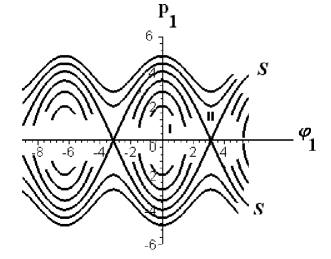
Figure 3: Phase portrait on the invariant manifold ${\cal M}_{1}$.

Dynamics upon ${\cal M}_{1}$ is governed by the two-dimensional system of equations

$$\left\{\begin{array}[]{lll}\dot{{\theta}}_{1}=&\frac{\displaystyle\partial H}{\displaystyle\partial p_{1}}=\frac{\displaystyle p_{1}}{\displaystyle 2mL^{2}}\\ &\\ \dot{p}_{1}=&-\frac{\displaystyle\partial H}{\displaystyle\partial q_{1}}=-2mgL\sin({\theta}_{1}).\\ \end{array}\right.$$ (20)

In Fig.3 each orbit has a definite total energy. The point I corresponds to the solution $(\theta_{1}=0,p_{1}=0)$, a pure center upon the invariant manifold. That indicates that the robot arms is standing still in the vertical position. Another saddle-center fixed point upon ${\cal M}_{1}$ is $(\theta_{1}=\pi,p_{1}=0)$. They correspond to the case where the $AB$ link of the robot arm (cf.Figs.1 and 2) remains in the vertical position (downwards and upwards, respectively), and only the $BC$ link is free to move.

III.2 The normal form of the Hamiltonian

The hamiltonian describing the dynamics in the linear neighborhood of a saddle-center can always be rewritten as the sum of a rotational energy term and a hyperbolic energy term. This is a consequence of Moser’s theorem moser , which establishes that in a sufficiently small neighborhood of any saddle-center point, there is a set of canonically conjugate variables so that the hamiltonian in that neighboorhood is separable into a purely rotational term, and a purely hyperbolic term. We will apply the method of normal forms to find this set of coordinates.

The method of normal formsosorio consists basically in applying Taylor series expansion to the velocity field around a fixed point. When such point is a saddle-center point, we may write the expanded hamiltonian in its quadratic (or normal) form. A canonical transformation is carried out so that we have vanishing off-diagonal termslandau . The transformation for the linear neighborhood of ${\cal P}_{2}$ is

$$\theta_{1} = x+y~{};$$ (21)

$$p_{1} = -\frac{2\left(5+\sqrt{17}\right)}{17+5\sqrt{17}}\left(\frac{2p_{x}}{5+\sqrt{17}}-\frac{\left(5+\sqrt{17}\right)p_{y}}{4}\right)~{};$$ (22)

$$\theta_{2}= \frac{\left(5+\sqrt{17}\right)}{4}x+\frac{2}{5+\sqrt{17}}y+\pi~{};$$ (23)

$$p_{2} = \frac{2\left(5+\sqrt{17}\right)}{17+5\sqrt{17}}\left(p_{x}-p_{y}\right).$$ (24)

In the new coordinates $(x,\,p_{x},\,y,\,p_{y})$, this fixed point is described by

$$\bar{{\cal P}_{2}}:(x=0,p_{x}=0,y=0,p_{y}=0).$$ (25)

Substituting (21)–(24) into the hamiltonian (1) and linearizing it in the neighborhood of $\bar{{\cal P}_{2}}$, it can be finally cast in its normal form

$$H=E_{hyp}+E_{rot}+\epsilon,$$ (26)

where

$$\epsilon=mgL$$ (27)

fixates the energy surface upon which the motion of the robot arm will take place. The energies

$$\left\{\begin{array}[]{lllll}E_{hyp}=&\frac{\displaystyle{\alpha}_{1}}{\displaystyle 2mL^{2}}p_{x}^{2}-\frac{\displaystyle mgL}{\displaystyle 2}{\alpha}_{3}x^{2},\\ &\\ E_{rot}=&\frac{\displaystyle{\alpha}_{2}}{\displaystyle 2mL^{2}}p_{x}^{2}+\frac{\displaystyle mgL}{\displaystyle 2}{\alpha}_{4}\left(y-\pi\right)^{2},\\ \end{array}\right.\\$$ (28)

correspond to the hyperbolic and rotational energies, respectively. The ${\alpha}_{l}^{\prime}$s are numerical positive coefficients originated from the canonical tranformation (21). Those coefficients can be found in appendix B. In the new coordinates, according to the hamiltonian (26), the linearized solutions around $\bar{{\cal P}_{2}}$ are

$$\left\{\begin{array}[]{llllll}x(t)\cong&\frac{\sqrt{2\left(3+\sqrt{17}\right)gL}\left(5+\sqrt{17}\right)}{68mgL^{2}}\left(c_{1}\exp({wt})-c_{2}\exp({-wt})\right)\\ &\\ p_{x}(t)\cong&{c_{1}\exp({wt})-c_{2}\exp({-wt})}\\ &\\ y(t)\cong&\frac{D_{2}\sqrt{2\left(\sqrt{17}-3\right)gL}\left(1+5\sqrt{17}\right)}{34mgL^{2}}\mbox{sen}\left(wt+\sigma\right)\\ &\\ p_{y}(t)\cong&D_{2}\cos\left(wt+\sigma\right)\\ \end{array}\right.$$ (29)

Notice that in this linear neighborhood the rotational and hyperbolic motions are totally uncoupled.In (29), $c_{1},\,c_{2},\,D_{2}$ and $\sigma$ are arbitray constants of integration, depending on the initial conditions. The frequency $w$ is related to the frequency $w_{0}$ by

$$w=\frac{\displaystyle\sqrt{2\left(\sqrt{17}-3\right)}}{\displaystyle 2}w_{0}.$$ (30)

Similar results are found for the remaining saddle-center fixed point ${\cal P}_{3}$, and we shall omit such discussion here. As to the pure center fixed point, it will be described in the new coordinates as $\bar{{\cal P}_{1}}:\,x=-\frac{\displaystyle 2\pi(5+\sqrt{17})}{\displaystyle 17+5\sqrt{17}},\,p_{x}=0,\,y=\frac{\displaystyle 2\pi(5+\sqrt{17})}{\displaystyle 17+5\sqrt{17}},\,p_{y}=0$.

The linearized solutions in the neighborhood of the pure center are

$$\left\{\begin{array}[]{llllll}x(t)\cong&\frac{\displaystyle-2D_{1}\sqrt{2\left(5+\sqrt{17}\right)gL}\left(17+5\sqrt{17}\right)}{\displaystyle 17mgL^{2}}\mbox{sen}\left(\Omega_{1}t+\theta\right)+\\ &\\ +&D_{2}\sqrt{2\left(5-\sqrt{17}\right)gL}\left(5\sqrt{17}-17\right)\mbox{sen}\left(\Omega_{2}t+\sigma\right)\\ &\\ p_{x}(t)\cong&-8D_{1}\left(4+\sqrt{17}\right)\cos\left(\Omega_{1}t+\theta\right)+\frac{D_{2}\left(4+\sqrt{17}\right)}{2}\cos\left(\Omega_{2}t+\sigma\right)\\ &\\ y(t)\cong&D_{1}\sqrt{2\left(5+\sqrt{17}\right)gL}\left(153+37\sqrt{17}\right)\mbox{sen}\left(\Omega_{1}t+\theta\right)+\\ &\\ +&D_{2}\frac{\sqrt{2\left(5-\sqrt{17}\right)gL}}{34mgL^{2}}\left(153+37\sqrt{17}\right)\mbox{sen}\left(\Omega_{2}t+\sigma\right)\\ &\\ p_{y}(t)\cong&2D_{1}\cos(\Omega_{1}t+\theta)+2D_{2}\cos(\Omega_{2}t+\sigma)\\ \end{array}\right.$$ (31)

where the frequencies

$$\Omega_{1}=\frac{\sqrt{2(5+\sqrt{17})}}{2}w_{0};\,\Omega_{2}=\frac{\sqrt{2(5-\sqrt{17})}}{2}w_{0},$$

are also related to the frequencies $w_{0}$.

As to the dynamics in the neighborhood of the pure-saddle fixed point ${\cal P}_{4}$, the solutions are linear combinations of real exponential functions. We shall restrict our discussion to the saddle-center fixed points, due to it rich topology.

III.3 Topology of the linear neighborhood of saddle-center

Let us now analyze all possible motions in the linear neighborhood of the saddle-center point. As we have seen, dynamics in this neighborhood is governed by the hamiltonian (26). Thus, there are three possibilities: (a) $E_{rot}\neq 0;\,E_{hyp}=0$; (b) $E_{rot}=0;\,E_{hyp}\neq 0$ and (c) $E_{rot}\neq 0;\,E_{hyp}\neq 0$. We will discuss each case separately.

(a) For $E_{rot}\neq 0,\,E_{hip}=0$, there are two possibilities:

1. If $(p_{x}=0,\,x=0)$, we have unstable periodic orbits $\tau$ upon the $(y,\,p_{y})$ plane, and their projection upon the $(x,\,p_{x})$ plane is the $(x=0,\,p_{x}=0)$ point. Such orbits depend continuously on the parameter $\epsilon$, so that

   $$E_{rot}=-mgL.$$ (32)

2. If $p_{x}=\pm mL\sqrt{\frac{\displaystyle{\alpha}_{3}g}{\displaystyle{\alpha}_{1}}}x$, the onedimensional linear manifolds $V_{S}$(stable) and $V_{i}$(unstable) (cf. Fig.4 and Fig.5) tangent the saddle-center are defined. The separatrices $S$ are non-linear extensions of $V_{S}$ and $V_{i}$. The general motion is the direct product of periodic orbits $\tau$ with the manifolds $V_{S}$ and $V_{i}$, generating the structures of cylinders $(\tau\times V_{S})$(stable) and $(\tau\times V_{i})$(unstable). Orbits on such cylinders have the periodic orbits $\tau$ as their assymptotic limit $(t\rightarrow\infty)$. Notice that those cylinders have the same energy as that of the unstable periodic orbits $\tau$.

Figure 4: Projection of orbits upon the $(y,P_{y})$ plane near $y=0$, corresponding to unstable periodic orbits in the neighborhood of the fixed point.

Figure 5: Projection of orbits upon the $(x,P_{x})$ plane near $x=0$, revealing the hyperbolic structure in the neighborhood of the fixed point.

(b) If $E_{rot}=0$ and $E_{hip}\neq 0$, the motion is upon the invariant manifold ${\cal M}$ defined by (18) or (19).

The resulting motion of the system consists in hyperbolic orbits on the $(x,\,p_{x})$ plane, as the projection of orbits on the $(y,\,p_{y})$ plane is reduced to a single point defined by (LABEL:xxc).

(c) If $E_{rot}\neq 0$ and $E_{hip}\neq 0$, the resultant motion is the direct product of hyperbolae related to the I, I^′, II and II^′ regions of Fig.5, with the periodic orbits on the $(y,\,p_{y})$ plane in the linear neigborhood of the saddle-center fixed point.

IV The robot arm with constant external torques

We will analyze now the case of non-null constant external torques. There are still four fixed points, namely,

$${\cal P}^{\prime}_{1}=\left(\begin{tabular}[]{c}$\arctan\left(\frac{\beta_{1}}{\sqrt{-\beta_{1}^{2}+4m^{2}g^{2}L^{2}}}\right)$\\ 0\\ $\arctan\left(\frac{\beta_{2}}{\sqrt{-\beta_{2}^{2}+m^{2}g^{2}L^{2}}}\right)$\\ 0\end{tabular}\right),\ \ {\cal P}^{\prime}_{2}=\left(\begin{tabular}[]{c}$\arctan\left(\frac{\beta_{1}}{\sqrt{-\beta_{1}^{2}+4m^{2}g^{2}L^{2}}}\right)$\\ 0\\ $\arctan\left(\frac{\beta_{2}}{-\sqrt{-\beta_{2}^{2}+m^{2}g^{2}L^{2}}}\right)$\\ 0\end{tabular}\right),$$ (33)

$${\cal P}^{\prime}_{3}=\left(\begin{tabular}[]{c}$\arctan\left(\frac{\beta_{1}}{-\sqrt{-\beta_{1}^{2}+4m^{2}g^{2}L^{2}}}\right)$\\ 0\\ $\arctan\left(\frac{\beta_{2}}{\sqrt{-\beta_{2}^{2}+m^{2}g^{2}L^{2}}}\right)$\\ 0\end{tabular}\right),\ \ {\cal P}^{\prime}_{4}=\left(\begin{tabular}[]{c}$\arctan\left(\frac{\beta_{1}}{-\sqrt{-\beta_{1}^{2}+4m^{2}g^{2}L^{2}}}\right)$\\ 0\\ $\arctan\left(\frac{\beta_{2}}{-sqrt{-\beta_{2}^{2}+m^{2}g^{2}L^{2}}}\right)$\\ 0\end{tabular}\right).$$ (34)

where $\beta_{1}$ and $\beta_{2}$ stand for the constant external torques. Coordinates, from top to bottom, are ordered according to $(\theta_{1},p_{1},\theta_{2},p_{2})$. The coordinates of those fixed points must be real; hence, their existence is subject to the two simultaneous conditions:

$$|\beta_{1}| \leq 2mgL,$$ (35)

$$|\beta_{2}| \leq mgL.$$ (36)

If those conditions are satisfied, there will be four fixed points, as in the null-torque case. The same procedure used previously to analyze the nature of such fixed points can be applied, and their nature determined. It turns out that for

$$|\beta_{1}| < 2mgL$$ (37)

$$|\beta_{2}| < mgL,$$ (38)

The nature of fixed points is the same for that in which the torques are null. In other words, ${\cal P}^{\prime}_{1}$ is a pure center, with corresponding energy

$$E_{1} = -\sqrt{\left(-\beta_{2}^{2}+m^{2}g^{2}L^{2}\right)}-\sqrt{-\beta_{1}^{2}+4m^{2}g^{2}L^{2}}+$$ (39)

$$-\arctan\left(\frac{\beta_{1}}{\sqrt{-\beta_{1}^{2}+4m^{2}g^{2}L^{2}}}\right)\beta_{1}-\arctan\left(\frac{\beta_{2}}{\sqrt{-\beta_{2}^{2}+m^{2}g^{2}L^{2}}}\right)\beta_{2}$$

In their turn, ${\cal P}^{\prime}_{2}$ and ${\cal P}^{\prime}_{3}$ are saddle-center points, with corresponding energy

$$E_{2} = -\sqrt{-\beta_{2}^{2}+m^{2}g^{2}L^{2}}+\sqrt{-\beta_{1}^{2}+4m^{2}g^{2}L^{2}}+$$ (40)

$$-\arctan\left(\frac{\beta_{1}}{-\sqrt{-\beta_{1}^{2}+4m^{2}g^{2}L^{2}}}\right)\beta_{1}-\arctan\left(\frac{\beta_{2}}{\sqrt{-\beta_{2}^{2}+m^{2}g^{2}L^{2}}}\right)\beta_{2}$$

and

$$E_{3} = \sqrt{-\beta_{2}^{2}+m^{2}g^{2}L^{2}}-\sqrt{-\beta_{1}^{2}+4m^{2}g^{2}L^{2}}+$$ (41)

$$-\arctan\left(\frac{\beta_{1}}{\sqrt{-\beta_{1}^{2}+4m^{2}g^{2}L^{2}}}\right)\beta_{1}-\arctan\left(\frac{\beta_{2}}{-\sqrt{-\beta_{2}^{2}+m^{2}g^{2}L^{2}}}\right)\beta_{2}$$

respectively. The fourth fixed point ${\cal P}^{\prime}_{4}$ is a pure saddle, with energy

$$E_{4} = \sqrt{-\beta_{2}^{2}+m^{2}g^{2}L^{2}}+\sqrt{-\beta_{1}^{2}+4m^{2}g^{2}L^{2}}+$$ (42)

$$-\arctan\left(\frac{\beta_{1}}{-\sqrt{-\beta_{1}^{2}+4m^{2}g^{2}L^{2}}}\right)\beta_{1}-\arctan\left(\frac{\beta_{2}}{-\sqrt{-\beta_{2}^{2}+m^{2}g^{2}L^{2}}}\right)\beta_{2}.$$

If $\beta_{1}=\beta_{2}=0$, we fall into the null torques case, and the classification of those points is the same. In the special case

$$|\beta_{2}|=mgL\mbox{ and }|\beta_{1}|=2mgL$$ (43)

it can be shown that all fixed points are degenerate, i.e., the jacobian matrices of the linearized system in the neighborhood of those fixed points have all vanishing eigenvalues. In this case, a new procedure must be taken, so that at first this degenerescence is raised, and then the points are classifiedbogo . We will not approach the degenerate case here.

From what has been seen above, the topology of orbits in the linear neighborhood of fixed points is the same for both the null-torques and non-null constant torques cases.

By the introduction of constant external torques, their intensity can be adjusted so that the robot arm be held any desired configuration in equilibrium. The majority of those equilibrium points are unstable, though: any fluctuation on the initial conditions can take the system out of equilibrium. In the case of the saddle-center points, the choice of certain branches of the saddle can lead to stable equilibrium, even in the presence of fluctuations.

V Conclusions and final remarks

We have proposed that the planar manipulator with two links and two rotational joins, a system with two degrees of freedom, be described by the hamiltonian of a double pendulum subject to two external torques. In its phase space, four fixed points (stationary solutions) can be found; a pure center, a pure saddle, and two saddle-centers, which can be used as a clue to the structure of orbits in in all phase space. We have also observed that there are two similar invariant manifolds, each one of them associated to a saddle-center points. The phase portrait of the system upon those manifolds resembles that of a mathematical pendulum of arbitrary amplitude. Dynamics upon such manifolds is governed by a unidimensional autonomous system, thus being totally integrable. For any set of initial conditions placed on one such manifold, the orbits will be confined to that manifold. We should keep in mind, however, that those manifolds are embedded into a four-dimensional phase space, so that the system in general in non-integrable.

An important result is that for constant external torques, the phase space topology in the linear neighborhood of the fixed points is the same as that of the null-torques case, if certain conditions involving the torques and parameters of the system are satisfied. With a proper choice of torque intensities, then, we may define any point in configuration space as a fixed point, without altering its nature, in relation to the null-torques case. In particular, the topology of orbits in the linear neighborhood of the saddle-center points is the same, as the existence of the corresponding invariant manifolds.

A possible continuation of this work involves the analysis of the non-linear neighborhood of fixed points. Strong indications of chaotic behavior are expected, due to the non-integrability of the system.

References

• (1) A. A. Shabana. Dynamics of Multibody Systems. U.S.A., John Willey & Sons, 1998.
• (2) P. Hagedorn. Oscilações Não-Lineares. São Paulo, Ed. Edgar Blücher, 1984.
• (3) L. Meirovitch. Analytical Methods in Vibrations. Canada, The Macmillan Company, 1967.
• (4) L. Landau, E. Lifschitz. Mecânica. Moscow, Mir, 1980.
• (5) G.A. Monerat, H.P. de Oliveira, I.D. Soares. Phys. Rev. D58(1998)063504.
• (6) M. A. Moser. Commum. Pure and Appl. Math. 11(1958)257.
• (7) A.M. Ozorio de Almeida. Sistemas Hamiltonianos, Caos e Quantização. 3${}^{rd}.$ ed. São Paulo, Unicamp, 1995.
• (8) H. P. de Oliveira, S. D. Soares, T. J. Stuchi. Phys. Rev.D56(1997)730.
• (9) O. I. Bogoyavlensky. Methods in the Qualitative Theory of Dynamical Systems in Astrophysics and Gas Dynamics. Springer-Verlarg, 1985.