Classes of Spatiotemporal Objects
and Their Closure Properties

Abstract

We present a data model for spatio-temporal databases. In this model spatio-temporal data is represented as a finite union of objects described by means of a spatial reference object, a temporal object and a geometric transformation function that determines the change or movement of the reference object in time.

We define a number of practically relevant classes of spatio-temporal objects, and give complete results concerning closure under Boolean set operators for these classes. Since only few classes are closed under all set operators, we suggest an extension of the model, which leads to better closure properties, and therefore increased practical applicability. We also discuss a normal form for this extended data model.

1 Introduction

Many natural or man-made phenomena have both a spatial and a temporal extent. Consider for example a forest fire, a meteorological event (e.g., the movement of clouds pressure areas), property histories in a city or the flight of an air plane. To store information about such phenomena in a database, appropriate data modeling constructs are needed.

In this paper, we introduce and discuss a general framework for specifying spatio-temporal data. Hereto, the new concept of spatio-temporal object is introduced. We represent a spatio-temporal object as a finite number of objects represented by means of a spatial reference object, a temporal object (i.e., a time interval) and a time-dependent geometric transformation that determines how this spatial object moves or changes through space during the considered time interval. Although this model is suited for data in arbitrary dimensions, we focus on two-dimensional reference objects that move or change during time.

In this framework, a number of classes of practically relevant spatio-temporal objects arise naturally. These classes are indexed by the type of spatial reference object and the type of transformation functions that are allowed. On the level of reference objects, we consider polygons, triangles, triangles with two sides parallel to the coordinate axes of the two-dimensional plane and rectangles with all sides parallel to the coordinate axes. We consider time-dependent affinities, scalings and translations for what concerns transformation functions. These functions can be expressed by rational, polynomial, respectively linear functions.

We investigate these classes with respect to closure under Boolean set operations, namely union, intersection and set-difference.

By definition, these classes are closed under union (a spatio-temporal object is described as the union of atomic objects). We call a class closed under intersection (respectively set-difference) if any finite intersection (respectively set-difference) of objects from a class can again be described by an object from that class (i.e., as a union of atomic objects). The classes that we consider are not necessarily closed under intersection and set-difference.

We provide an in-depth and exhaustive study of their closure with respect to all set-theoretic operations, and we conclude that our model for representing spatio-temporal data gives very poor closure results for the classes of objects we considered important for spatio-temporal practice. The only classes that seems to be useful in this respect have polygons as spatial reference objects and use rational affinities to move or change these objects in time.

A conclusion is that we have to enrich the data model by allowing set-theoretic operations other than union in the construction of geometric objects from atomic geometric objects. As soon as we also allow spatio-temporal objects to be constructed from atomic ones by means of union and intersection (or union and set-difference) then the model becomes closed for all Boolean set operations. Indeed, as an important result, we show that our classes, that are drawn from practice, have the nice property that they are closed under intersection if and only if they are closed under set-difference.

To appreciate the need for applying set-theoretic operators to spatiotemporal objects, consider the following scenario. Let two spatial objects represent the extents of the safe areas around two different ships. Taking into account the movement of ships, the extents of the safe areas over a period of time can be represented as two spatiotemporal objects. To avoid collisions, one needs to be able to determine the intersection of those objects.

The substantial literature on spatial and temporal databases does not provide much guidance in dealing with spatiotemporal phenomena. Spatial databases [20] deal with spatial objects (e.g., rectangles or polygons) and temporal databases [17] with temporal ones (e.g., time intervals). Their combination can handle discrete change [19] but not continuous change, which is required by applications dealing with phenomena like movement, natural disasters, or the growth of urban areas. In the latter applications, the temporal and spatial aspects cannot be conveniently separated.

Spatiotemporal data models and query languages are a topic of growing interest. The need to model both discrete and continuous change has been identified. The issue of closure under Boolean set operations has also received in this context a considerable attention. This is not surprising, since, for example, closure under intersection is essential for spatiotemporal join.

The paper [19] presents one of the first such models. However, it is only capable of modeling discrete change.

In [6] the authors define in an abstract way moving points and regions. Apart from moving points, no other classes of concrete, database-representable spatiotemporal objects are defined. In that approach continuous movement (but not growth or shrinking) can be modeled using linear interpolation functions. In the subsequent paper [7], the authors discuss a concrete, polyhedral representation of moving, growing and shrinking regions, which is applicable only to significantly restricted classes of spatiotemporal objects. This guarantees closure but eliminates the possibility of representing scaling and more general transformations. The results of the present paper shed some light on when similar concrete representations exist and when they do not.

In [9] the authors propose a formal spatiotemporal data model based on constraints in which, like in [19], only discrete change can be modeled. An SQL-based query language is also presented.

We have proposed elsewhere [5] a spatiotemporal data model based on parametric polygons: polygons whose vertices are defined using linear functions of time. This model is also capable of modeling continuous change but is not closed under intersection. A variation of this model restricted to rectangles but extended with periodic functions is given in [3]. The latter model is closed under set theoretic operators, enabling the definition of an extended relational algebra query language, for which query evaluation can be done in PTIME in the size of the input spatiotemporal database. The closure properties for [5] and [3] seem analoguous to the closure properties of the framework presented in this paper, respectively, but the relationships among these frameworks needs to be further explored.

Both discrete and continuous change can be represented using constraint databases [12]. Compared to the latter technology, our approach seems more constructive and amenable to implementation using standard database techniques. On the other hand, constraint databases do not suffer from the lack of closure under intersection. To some degree, it is due to the fact that the intersection of two generalized tuples in constraint databases need not immediately computed but rather the tuples may be only conjoined together. In most implementations of constraint databases [2, 10, 15] the “real” computation of the intersection occurs during projection or the presentation of the query result to the user. It is unclear whether such a strategy offers any computational advantages over the approach in which the intersections are computed immediately. In fact, recent work on spatial constraint databases [13] proposes extensions to relational algebra that require immediate computations of spatial object intersections. Also, our approach is potentially more general than constraint databases. For example, by moving beyond rational functions (but keeping the same basic framework) we can represent rotations with a fixed center. Finally, in our model it is easy to obtain any snapshot of a spatiotemporal object, making tasks like animation straightforward. It is not so in constraint databases where geometric representations of snapshots have to be explicitly constructed from constraints [4].

This paper is organized as follows: In Section 2, we give definitions and describe the relevant classes of spatio-temporal objects. The closure results for these classes with respect to Boolean set operations are given in Section 3. We propose the extended model in Section 4 and describe a normal form for objects in this extended model. Section 5 gives comments and concludes the paper.

2 Definitions and preliminaries

In this section, we define the notion of spatio-temporal object. In our approach, a spatio-temporal object consists of a spatial reference object, a time interval during which the spatio-temporal object exists and a continuous transformation that defines how the spatial reference object moves and changes during the interval of time.

2.1 Spatio-temporal and geometric objects

Let ${\rm{\bf R}}$ be the set of real numbers and ${\rm{\bf R}}^{2}$ be the $2$-dimensional real plane.

Definition 2.1

A spatial object is a subset of ${\rm{\bf R}}^{2}$. A temporal object is a subset of ${\rm{\bf R}}$ (we assume a single temporal dimension). A spatio-temporal object is a subset of ${\rm{\bf R}}^{2}\times{\rm{\bf R}}$.     $\sqcap$$\sqcup$

These definitions are very general and disregard the fact that objects should be finitely representable in the computer’s memory. In this paper, we will study more restricted classes of spatial and spatio-temporal objects that are important from a practical point of view and have simple and efficient representations. Such classes have been identified in the course of spatial and spatio-temporal database research.

Here, we propose a geometric approach: a spatio-temporal object is defined as a spatial reference object together with a continuous transformation that defines how the object moves or changes during some time interval.

Definition 2.2

An atomic geometric object $\cal O$ is a triple $(S,I,f)$, where

• $S\subset{\rm{\bf R}}^{2}$ is the spatial reference object of $\cal O$, which is semi-algebraic in ${\rm{\bf R}}^{2}$;

• $I\subset{\rm{\bf R}}$ is the time domain of $\cal O$, which is a connected and bounded semi-algebraic set in ${\rm{\bf R}}$ (i.e., a point or a bounded interval); and

• $f:{\rm{\bf R}}^{2}\times{\rm{\bf R}}\rightarrow{\rm{\bf R}}^{2}$ is the transformation function of $\cal O$, which is semi-algebraic and continuous both in the time coordinate and in the spatial coordinates.

The semantics of an atomic geometric object ${\cal O}=(S,I,f)$ is the spatio-temporal object $st({\cal O})=\{(x,y;t)\in{\rm{\bf R}}^{2}\times{\rm{\bf R}}\mid(\exists x^{\prime})(\exists y^{\prime})((x^{\prime},y^{\prime})\in S\mathrel{\land}t\in I\mathrel{\land}(x,y)=f(x^{\prime},y^{\prime};t))\}.$     $\sqcap$$\sqcup$

We remark that this definition guarantees that there is a finite representation of an atomic geometric object by means of the polynomial inequalities that describe its reference object, its time domain and the graph of its transformation function. This means that this data model is within the constraint model for databases (we refer to [14] for an overview of the research results in this area).

Definition 2.3

A geometric object is a finite set of atomic geometric objects. The semantics of a geometric object $\{{\cal O}_{1},\ldots,{\cal O}_{n}\}$ is the union of the semantics of the atomic objects that constitute it, i.e., the set

$$\bigcup_{1\leq i\leq n}st({\cal O}_{i}).$$

$\sqcap$$\sqcup$

We agree that whenever we write “the spatio-temporal object $\cal O$”, where $\cal O$ is an (atomic) geometric object, we mean the semantics of the (atomic) geometric object $\cal O$. Also, when ${\cal O}=(S,I,f)$ is an atomic object and $t\in I$, we will refer to the set $\{(x,y)\mid(\exists x^{\prime})(\exists y^{\prime})((x^{\prime},y^{\prime})\in S\land(x,y)=f(x^{\prime},y^{\prime},t))\}$ as the frame of ${\cal O}$ at time $t$ and we will denote it $f(S;t)$.

We define the time domain of a geometric object to be the smallest time interval that contains all the time domains of the composing atomic geometric objects. Recall that the smallest interval containing a set of intervals is also known as the convex closure of this set. We denote the convex closure of the sets $I_{1}$, $I_{2}$, …, $I_{n}$ by $\overline{\bigcup}_{i=1}^{n}I_{i}$.

Remark that a spatio-temporal object is empty (or non-existing) outside the time domain of the geometric object that defines it. Also, within its time domain a spatio-temporal object can be empty (for instance, at any moment when no atomic geometric object exists).

We conclude this section by remarking that the above introduced notions of spatial and spatio-temporal object and of (atomic) geometric object can be generalized to arbitrary dimension $d$ (by simply substituting $d$ for $2$ in the above definitions). Since all the results in this paper are formulated for dimension 2, we have chosen not to use this generalization here.

2.2 Practically relevant classes of geometric objects

Here, we define special classes of geometric objects that are relevant to spatio-temporal database practice. These classes are denoted by

$$\langle{\cal S,F}\rangle$$

and they are determined by the type $\cal S$ of spatial reference object and the type $\cal F$ of transformation function. For clarity, a geometric object belongs to a class if all of its atomic geometric objects belong to that class.

The classes of geometric figures in the plane ${\rm{\bf R}}^{2}$ that we will consider are

• ${\cal S}_{\rm Poly}$, the class of arbitrary polygons,

• ${\cal S}_{\rm Tr}$, the class of arbitrary triangles,

• ${\cal S}_{\rm TrAx}$, the class of triangles with two sides parallel to the coordinate axes, and

• ${\cal S}_{\rm Rect}$ the class of rectangles with all sides parallel to the coordinate axes.

In this paper, we assume triangles, polygons and rectangles to be filled objects. But since we allow two or more corner points of a triangle or rectangle to coincide, the model can deal with polylines and points too. A line segment and a point are considered triangles. Also line segments parallel to the axes and points are considered rectangles. Finally, note that ${\cal S}_{\rm Rect}\subset{\cal S}_{\rm TrAx}\subset{\cal S}_{\rm Tr}\subset{\cal S}_{\rm Poly}$.

The classes of transformation functions we will consider are

• ${\cal F}_{\rm Aff}$, the class of the affine transformations,

• ${\cal F}_{\rm Sc}$, the class of the scalings,

• ${\cal F}_{\rm Trans}$, the class of the translations, and

• ${\cal F}_{\rm id}$, the class consisting of the identity mapping.

It is clear that ${\cal F}_{\rm id}$, ${\cal F}_{\rm Trans}$ and ${\cal F}_{\rm Sc}$ are subclasses of ${\cal F}_{\rm Aff}$. More technically, these classes are defined as follows. The class ${\cal F}_{\rm Aff}$ of affine transformations consists of the mappings ${\rm{\bf R}}^{2}\times{\rm{\bf R}}\rightarrow{\rm{\bf R}}^{2}$ of the form

$$(x,y;t)\mapsto\left(\!\begin{array}[]{@{}cc@{}}a(t)&b(t)\\ c(t)&d(t)\end{array}\!\right)\left(\!\begin{array}[]{@{}c@{}}x\\ y\end{array}\!\right)+\left(\!\begin{array}[]{@{}c@{}}e(t)\\ f(t)\end{array}\!\right),$$

where $a$, $b$, $c$, $d$, $e$, and $f$ are function from ${\rm{\bf R}}$ to ${\rm{\bf R}}$ with $a(t)d(t)-c(t)b(t)\not=0$ for all $t$ in the relevant time domain.

The class ${\cal F}_{\rm Sc}$  of scalings consists of the affine transformations for which the functions $b$ and $c$ are identical to 0. The class ${\cal F}_{\rm Trans}$ consists of the scalings for which the functions $a$ and $d$ are identical to 1.

For practical purposes we will only consider functions $a$, $b$, $c$, $d$, $e$, and $f$ that are semi-algebraic and continuous as required by the definition. These are

• the rational functions (i.e., fractions of polynomial functions),

• the polynomial functions and

• the linear polynomial functions.

The corresponding classes of transformations will be denoted using superscripts ${\cal F}^{\rm Rat}$, ${\cal F}^{\rm Poly}$, and ${\cal F}^{\rm Lin}$. For example, ${\cal F}_{\rm Sc}^{\rm Rat}$ represents the class of rational scalings. We assume that the time domain of an atomic geometric object belongs to the domain of the transformation function and that the denominator of a rational function in the definition of a transformation is never zero in the closure of the time domain (thus, the moving figure will remain within fixed bounds during the time domain).

Note that the shape of a spatio-temporal object at a certain time instant is not necessarily the same as the shape of the reference object of the geometric object that gives rise to the spatio-temporal object. For example, a rectangle is mapped to a parallelogram under an affinity.

2.3 Example

Let ${\cal O}_{A}=(S_{A},I_{A},f_{A})$ and ${\cal O}_{B}=(S_{B},I_{B},f_{B})$ be two (atomic) geometric objects with spatial reference objects $S_{A}$ and $S_{B}$ respectively the triangles with corner points $(-1,0)$, $(1,0)$, $(0,1)$ and $(-1,0)$, $(1,0)$, $(0,-1)$, and time domains $I_{A}=I_{B}=[0,2]$. In this time domain, $S_{A}$ remains at its place (i.e., $f_{A}(x,y;t)=(x,y)$ for all $t$), while $S_{B}$ is translated with constant speed (equal to 1) in the direction of the positive $y$-axis (i.e., $f_{B}(x,y;t)=(x,y+t)$. The functions $f_{A}$ and $f_{B}$ belong to ${\cal F}^{\rm Lin}_{\rm Trans}$.

At $t=0$ both objects intersect in a line segment. For $0<t<1$ they intersect in a hexagon, for $1\leq t<2$ in a quadrangle, and finally for $t=2$ in a point.

Figure 1: Two atomic geometric objects. The time domain can be partitioned in four parts such that the intersection of the two objects retains the same shape during each element of the partition.

3 Closure properties under Boolean set operations

In this section, we work with the classes $\langle{\cal S,F}\rangle$ introduced in the previous section, and we investigate which of these classes $\langle{\cal S,F}\rangle$ are closed under the Boolean set operations $\cup$ (union), $\cap$ (intersection) and $\setminus$ (set difference). We first define what closure means.

Definition 3.1

Let $\theta$ be one of the operations $\cup$, $\cap$ or $\setminus$. We say that the class $\langle{\cal S,F}\rangle$ is (atomically) closed under $\theta$ if for any two (atomic) geometric objects ${\cal O}_{1}$ and ${\cal O}_{2}$ in $\langle{\cal S,F}\rangle$ there exists a geometric object $\cal O$ in $\langle{\cal S,F}\rangle$ such that $st({\cal O})=st({\cal O}_{1})\mathrel{\theta}st({\cal O}_{2})$.     $\sqcap$$\sqcup$

We will refer to an object $\cal O$ that satisfies the condition in the definition as an intersection, union or difference of ${\cal O}_{1}$ and ${\cal O}_{2}$ (they need not be unique).

For the union operation, the closure follows immediately from the definition.

Property 3.1

For any class of objects $\cal S$ and any class of transformations $\cal F$, $\langle{\cal S,F}\rangle$ is closed under $\cup$.     $\sqcap$$\sqcup$

For $\cap$ and $\setminus$ the situation is more complicated. The next theorem is the main result that we want to prove in this section. It summarizes the closure results for intersection and set-difference.

Theorem 3.1

For any class of objects $\cal S$ among ${\cal S}_{\rm Poly}$, ${\cal S}_{\rm Tr}$, ${\cal S}_{\rm TrAx}$ and ${\cal S}_{\rm Rect}$ and any class of transformations $\cal F$ among ${\cal F}_{\rm Aff}$, ${\cal F}_{\rm Sc}$, ${\cal F}_{\rm Trans}$ and ${\cal F}_{\rm id}$, the closure with respect to $\cap$ and $\setminus$ is summarized in the following table.

$\cap$, $\setminus$	${\cal F}_{\rm Aff}^{\rm Rat}$	${\cal F}_{\rm Aff}^{\rm Poly}$	${\cal F}_{\rm Aff}^{\rm Lin}$	${\cal F}_{\rm Sc}^{\rm Rat}$	${\cal F}_{\rm Sc}^{\rm Poly}$	${\cal F}_{\rm Sc}^{\rm Lin}$	${\cal F}_{\rm Trans}^{\rm Rat}$	${\cal F}_{\rm Trans}^{\rm Poly}$	${\cal F}_{\rm Trans}^{\rm Lin}$	${\cal F}_{\rm id}$
${\cal S}_{\rm Poly}$	$+$	$-$	$-$	$-$	$-$	$-$	$-$	$-$	$-$	$+^{\dagger}$
${\cal S}_{\rm Tr}$	$+$	$-$	$-$	$-$	$-$	$-$	$-$	$-$	$-$	$+^{\dagger}$
${\cal S}_{\rm TrAx}$	$+$	$-$	$-$	$-$	$-$	$-$	$-$	$-$	$-$	$-$
${\cal S}_{\rm Rect}$	$+$	$-$	$-$	$+$	$+$	$+$	$-$	$-$	$-$	$+$

Closure is indicated by a $+$ sign, non-closure by a $-$ sign.     $\sqcap$$\sqcup$

The items marked with $\dagger$ are from [19].

The remainder of this section is devoted to proving this theorem. We do this by first proving some lemmas in a first subsection that reduce the number of cases that have to be looked at and by then proving the remaining cases in a second subsection.

3.1 Reduction properties

The properties in this section reduce the number of cases that have to be investigated. First, we give a set-theoretic lemma that will be used frequently.

Lemma 3.1

Let $A_{1},\ldots,A_{n}$ and $B_{1},\ldots,B_{m}$ be sets. Then

1. $(\bigcup_{i=1}^{n}A_{i})\cap(\bigcup_{j=1}^{m}B_{j})=\bigcup_{i=1}^{n}\bigcup_{j=1}^{m}(A_{i}\cap B_{j})$,

2. $(\bigcup_{i=1}^{n}A_{i})\setminus(\bigcup_{j=1}^{m}B_{j})=\bigcup_{i=1}^{n}((\cdots((A_{i}\setminus B_{1})\setminus B_{2})\setminus\cdots)\setminus B_{m})$

Proof. The first equality follows directly from distributivity of intersection with respect to union.

The second equality can be proven by induction on $m$, using the observation that $(\bigcup_{i=1}^{n}A_{i})\setminus B=(\bigcup_{i=1}^{n}A_{i})\cap B^{c}=\bigcup_{i=1}^{n}(A_{i}\cap B^{c})=\bigcup_{i=1}^{n}(A_{i}\setminus B)$, where $B^{c}$ denotes the complement of $B$ with respect to some universe.     $\sqcap$$\sqcup$

The next property says that for $\cap$ and $\setminus$ closure and closure on atomic objects coincide.

Property 3.2 (Atomicity)

Let $\cal S$ be a class of objects and $\cal F$ a class of transformations. Then

1. $\langle{\cal S,F}\rangle$ is closed under $\cap$ if and only if it is atomically closed under $\cap$, and

2. $\langle{\cal S,F}\rangle$ is closed under $\setminus$ if and only if it is atomically closed under $\setminus$.

Proof. Both for (a) and (b) the only-if direction is obvious. So we concentrate on the if-direction.

For the if-direction of (a), assume that $\langle{\cal S,F}\rangle$ is atomically closed under $\cap$ and let $\{{\cal O}_{1,1},{\cal O}_{1,2},\ldots,\allowbreak{\cal O}_{1,n}\}$ and $\{{\cal O}_{2,1},\allowbreak{\cal O}_{2,2},\allowbreak\ldots,{\cal O}_{2,m}\}$ be two geometric objects from $\langle{\cal S,F}\rangle$. By using Lemma 3.1 (a), we get

$$(\bigcup_{i=1}^{n}st({\cal O}_{1,i}))\cap(\bigcup_{j=1}^{m}st({\cal O}_{2,j}))=\bigcup_{i=1}^{n}\bigcup_{j=1}^{m}(st({\cal O}_{1,i})\cap st({\cal O}_{2,j})).$$

Since $\cap$ is assumed to be atomically closed, each $st({\cal O}_{1,i})\cap st({\cal O}_{2,j})$ can be written as a union $\bigcup_{k=1}^{l_{ij}}st({\cal O}_{k,i,j})$, where each ${\cal O}_{k,i,j}$ is an atomic geometric object. Therefore, the intersection of $\{{\cal O}_{1,1},{\cal O}_{1,2},\ldots,{\cal O}_{1,n}\}$ and $\{{\cal O}_{2,1},{\cal O}_{2,2},\ldots,{\cal O}_{2,m}\}$ can also be written as $\bigcup_{i=1}^{n}\bigcup_{j=1}^{m}\bigcup_{k=1}^{l_{i,j}}st({\cal O}_{k,i,j})$. This completes the proof of the if-direction of (a).

For the if-direction of (b), assume that $\langle{\cal S,F}\rangle$ is atomically closed under $\setminus$ and let $\{{\cal O}_{1,1},{\cal O}_{1,2},\allowbreak\ldots,\allowbreak{\cal O}_{1,n}\}$ and $\{{\cal O}_{2,1},\allowbreak{\cal O}_{2,2},\allowbreak\ldots,\allowbreak{\cal O}_{2,m}\}$ be two geometric objects from $\langle{\cal S,F}\rangle$. By using Lemma 3.1 (b), we get

$$(\bigcup_{i=1}^{n}st({\cal O}_{1,i}))\setminus(\bigcup_{j=1}^{m}st({\cal O}_{2,j}))=\bigcup_{i=1}^{n}((\cdots((st({\cal O}_{1,i})\setminus st({\cal O}_{2,1}))\setminus st({\cal O}_{2,2}))\setminus\cdots)\setminus st({\cal O}_{2,m})).$$

We prove, by induction on $m$, that $((\cdots((st({\cal O}_{1,i})\setminus st({\cal O}_{2,1}))\setminus st({\cal O}_{2,2}))\setminus\cdots)\setminus st({\cal O}_{2,m}))$ is of the form $\bigcup_{k=1}^{l}st({\cal O}^{\prime}_{k})$. Since $\setminus$ is assumed to be atomically closed, $st({\cal O}_{1i})\setminus st({\cal O}_{21})$ can be written as a union $\bigcup_{k=1}^{l_{1}}st({\cal O}^{\prime}_{k})$, where each ${\cal O}^{\prime}_{k}$ is an atomic geometric object. This proves the case $m=1$. Next, assume we have shown that $((\cdots((st({\cal O}_{1,i})\setminus st({\cal O}_{2,1}))\setminus st({\cal O}_{2,2}))\setminus\cdots)\setminus st({\cal O}_{2,m-1}))$ is $\bigcup_{k=1}^{l}st({\cal O}^{\prime}_{k})$ with all ${\cal O}^{\prime}_{k}$ atomic geometric objects. Then $((\cdots((st({\cal O}_{1,i})\setminus st({\cal O}_{2,1}))\setminus st({\cal O}_{2,2}))\setminus\cdots)\setminus st({\cal O}_{2,m}))$ is $(\bigcup_{k=1}^{l}st({\cal O}^{\prime}_{k}))\setminus st({\cal O}_{2,m})$, which is $\bigcup_{k=1}^{l}(st({\cal O}^{\prime}_{k})\setminus st({\cal O}_{2,m}))$, using Lemma 3.1 (b). Again, since $\setminus$ is assumed to be atomically closed, each of the sets $st({\cal O}^{\prime}_{k})\setminus st({\cal O}_{2,m})$ is of the form $\bigcup_{r=1}^{l_{k}}st({\cal O}^{\prime\prime}_{r})$. Therefore, the set-difference of $\{{\cal O}_{1,1},{\cal O}_{1,2},\ldots,{\cal O}_{1,n}\}$ and $\{{\cal O}_{2,1},{\cal O}_{2,2},\ldots,{\cal O}_{2,m}\}$ is also the semantics of a geometric object from $\langle{\cal S,F}\rangle$. This completes the proof.     $\sqcap$$\sqcup$

The following property states that intersection and set-difference are equivalent with respect to closure.

Property 3.3 (Equivalence of $\cap$ and $\setminus$)

Let $\cal S$ be a class of objects and $\cal F$ a class of transformations. Then $\langle{\cal S,F}\rangle$ is closed under $\cap$ if and only if it is closed under $\setminus$.

Proof. By Property 3.2 it suffices to prove this property for atomic geometric objects.

For the if-direction, assume that $\langle{\cal S,F}\rangle$ is closed under $\setminus$ and let ${\cal O}_{1}$ and ${\cal O}_{2}$ be two atomic geometric objects from $\langle{\cal S,F}\rangle$. Since,

$$st({\cal O}_{1})\cap st({\cal O}_{2})=(st({\cal O}_{1})\cup st({\cal O}_{2}))\setminus((st({\cal O}_{1})\setminus st({\cal O}_{2}))\cup(st({\cal O}_{2})\setminus st({\cal O}_{1})))$$

and since $(st({\cal O}_{1})\setminus st({\cal O}_{2}))$ and $(st({\cal O}_{2})\setminus st({\cal O}_{1}))$ are by assumption $\bigcup_{i=1}^{n}st({\cal O}^{\prime}_{i})$ respectively $\bigcup_{j=1}^{n}st({\cal O}^{\prime\prime}_{j})$ with all ${\cal O}^{\prime}_{i}$ and ${\cal O}^{\prime\prime}_{j}$ atomic geometric objects. Therefore, $st({\cal O}_{1})\cap st({\cal O}_{2})$ equals $((\cdots(st({\cal O}_{2})\setminus st({\cal O}^{\prime}_{1}))\setminus\cdots)\setminus st({\cal O}^{\prime}_{n}))\cup((\cdots(st({\cal O}_{2})\setminus st({\cal O}^{\prime\prime}_{1}))\setminus\cdots)\setminus st({\cal O}^{\prime\prime}_{m}))$, using Lemma 3.1 (b). Using the argumentation from the proof of the if-direction of (b) of Property 3.2, we can show that this set is again a union of semantics of atomic geometric objects from $\langle{\cal S,F}\rangle$.

For the only-if direction, assume that $\langle{\cal S,F}\rangle$ is closed under $\cap$ and let ${\cal O}_{1}=(S_{1},I_{1},f_{1})$ and ${\cal O}_{2}=(S_{2},I_{2},f_{2})$ be two atomic geometric objects from $\langle{\cal S,F}\rangle$. We have to show that $st({\cal O}_{1})\setminus st({\cal O}_{2})$ can be written as $\bigcup_{i=1}^{n}st({\cal O}^{\prime}_{i})$, with ${\cal O}^{\prime}_{i}$ atomic geometric objects. We can restrict our attention to the set $st({\cal O}_{1})\setminus st({\cal O}_{2})$ in the interval $I_{1}\cap I_{2}$ rather than in the complete interval $I_{1}\overline{\cup}I_{2}$ (since the set-difference is empty in $I_{2}\setminus I_{1}$ and equal to ${\cal O}_{1}$ in $I_{1}\setminus I_{2}$). Let $I$ denote the topological closure of $I_{1}\cap I_{2}$. The set $S_{B}=\{(x,y)\in{\rm{\bf R}}^{2}\mid(\exists x^{\prime})(\exists y^{\prime})(\exists t)((x^{\prime},y^{\prime})\in S_{1}\mathrel{\land}t\in I\mathrel{\land}f_{1}(x^{\prime},y^{\prime},t)=f_{2}(x,y;t))\}$ is compact (i.e., topologically closed and bounded) since it is the image of the compact set $S_{1}\times I$ under the continuous function $f_{2}^{-1}\circ f_{1}$. Therefore, also $S=S_{2}\cup S_{B}$ is a compact set in ${\rm{\bf R}}^{2}$. Let $\alpha:(x,y)\mapsto(ax+b_{1},ay+b_{2})$ be a scaling followed by a translation that maps $S_{2}$ to a set that strictly contains $S$ (this is possible since $S$ is bounded). Remark that $\alpha$ maps any line to a parallel line. Let ${\cal O}_{3}$ be the atomic geometric object $(\alpha(S_{2}),I,f_{2})$. At any moment $t$ in $I$, we thus have that $f_{2}(S_{2};t)\subset f_{2}(\alpha(S_{2});t)$ (since affinities are monotone mappings) and $f_{1}(S_{1};t)\subset f_{2}(\alpha(S_{2});t)$. Therefore, $st({\cal O}_{1})\setminus st({\cal O}_{2})=st({\cal O}_{1})\cap(st({\cal O}_{3})\setminus st({\cal O}_{2}))$.

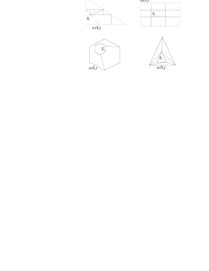
Figure 2: Examples of partitions of the set $\alpha(S_{2})\setminus S_{2}$ for the classes ${\cal S}_{\rm Poly}$, ${\cal S}_{\rm Tr}$, ${\cal S}_{\rm TrAx}$, and ${\cal S}_{\rm Rect}$ respectively.

Now, $st({\cal O}_{3})\setminus st({\cal O}_{2})$ can always be written as the semantics of a geometric object in $\langle{\cal S,F}\rangle$ where $\cal S$ and $\cal F$ are any pairs allowed in Theorem 3.1. For each of the classes ${\cal S}_{\rm Poly}$, ${\cal S}_{\rm Tr}$, ${\cal S}_{\rm TrAx}$, and ${\cal S}_{\rm Rect}$ this is illustrated in Figure 2. For each of these classes $\alpha(S_{2})\setminus S_{2}$ can be partitioned into a finite number of reference objects $T_{1}$, …, $T_{n}$ from these classes. So, define the atomic geometric objects ${\cal O}^{\prime}_{i}=(T_{i},I,f_{2})$ ($1\leq i\leq n$). Then $st({\cal O}_{3})\setminus st({\cal O}_{2})=\bigcup_{i=1}^{n}st({\cal O}^{\prime}_{i})$. Therefore, $st({\cal O}_{1})\cap(st({\cal O}_{3})\setminus st({\cal O}_{2}))=st({\cal O}_{1})\cap\bigcup_{i=1}^{n}st({\cal O}^{\prime}_{i})=\bigcup_{i=1}^{n}(st({\cal O}_{1})\cap st({\cal O}^{\prime}_{i}))$. Since we have assumed that $\langle{\cal S,F}\rangle$ is closed for intersection, the intersections $st({\cal O}_{1})\cap st({\cal O}^{\prime}_{i})$ can be written as $\bigcup_{k=1}^{l_{i}}st({\cal O}^{\prime\prime}_{k})$ with ${\cal O}^{\prime\prime}_{k}$ atomic geometric objects from $\langle{\cal S,F}\rangle$. Therefore also $st({\cal O}_{1})\cap(st({\cal O}_{3})\setminus st({\cal O}_{2}))$ can be written as such a union. This completes the proof.     $\sqcap$$\sqcup$

A final reduction property says that the closure results for polygons and triangles coincide. We can therefore concentrate on triangles further on.

Property 3.4

Let $\cal F$ be a class of transformations, and let $\theta$ be one of the operations $\cup$, $\cap$ or $\setminus$. Then $\langle{\cal S}_{\rm Poly},{\cal F}\rangle$ is closed under $\theta$ if and only if $\langle{\cal S}_{\rm Tr},{\cal F}\rangle$ is closed under $\theta$.

Proof. This property follows from the fact that any atomic geometric object ${\cal O}=(S,I,f)$ from $\langle{\cal S}_{\rm Poly},{\cal F}\rangle$ corresponds to a geometric object from $\langle{\cal S}_{\rm Tr},{\cal F}\rangle$. Indeed, let $T_{1},\ldots,T_{n}$ be an arbitrary triangulation of the polygon $S$. The geometric object $\{{\cal O}_{1},\ldots,{\cal O}_{n}\}$ with ${\cal O}_{i}=(T_{i},I,f)$ ($1\leq i\leq n$) has the same semantics as ${\cal O}=(S,I,f)$.

So, if $\langle{\cal S}_{\rm Poly},{\cal F}\rangle$ is closed under $\theta$, then also any union, intersection or set-difference of two elements of $\langle{\cal S}_{\rm Tr},{\cal F}\rangle$ is again a geometric object of $\langle{\cal S}_{\rm Poly},{\cal F}\rangle$ and because of the above argument also of $\langle{\cal S}_{\rm Tr},{\cal F}\rangle$.

On the other hand, suppose that $\langle{\cal S}_{\rm Tr},{\cal F}\rangle$ is closed under $\theta$. If ${\cal O}_{1}$ and ${\cal O}_{2}$ are objects in $\langle{\cal S}_{\rm Poly},{\cal F}\rangle$, then so are their union, intersection or set-difference, since they are in $\langle{\cal S}_{\rm Tr},{\cal F}\rangle$, which is a subclass of $\langle{\cal S}_{\rm Poly},{\cal F}\rangle$.     $\sqcap$$\sqcup$

3.2 Closure and non-closure proofs

In this section, we complete the proof of Theorem 3.1, by means of a series of lemmas that cover all the cases presented in the matrix of Theorem 3.1. Here, we take the reduction results of the previous section into account. In particular, we only consider intersections or set-differences of atomic geometric objects, and we do not have to consider polygons any more.

3.2.1 Finite time partition

Before giving these lemmas we introduce the technical notion of finite time partition. This will be of use in many of the proofs in this section. The finite time partition property tells us how and when the form (or appearance) of the intersection or set-difference of two atomic geometric objects changes. We observe that the intersection of two moving triangles can be empty, a single point, a straight line segment, a triangle, a quadrangle, a pentagon and a hexagon. The intersection of two moving rectangles can be empty, a single point, a line segment or a rectangle. We refer to all these different forms of the intersection or the set-difference as their possible shapes. Also the difference of two triangles or two rectangles can take a finite number of different shapes. In the example in Figure 1, the intersection takes four different shapes, whereas the difference takes five different shapes.

We define this notion now more technically. Let ${\cal O}_{1}=(S_{1},I_{1},f_{1})$ and ${\cal O}_{2}=(S_{2},I_{2},f_{2})$ be two atomic geometric objects with rational affine transformations with time domains $I_{1}$ and $I_{2}$. In the following, we denote by $I_{1}\mathbin{\overline{\cup}}I_{2}$ the convex closure of the set $I_{1}\cup I_{2}$ in ${\rm{\bf R}}$. Let $t$ be in $I_{1}\mathbin{\overline{\cup}}I_{2}$. Firstly, we call any line that intersects the border of $f_{i}(S_{i};t)$ in infinitely many points, a carrier of the frame $f_{i}(S_{i};t)$ and denote it $car(f_{i}(S_{i};t))$ ($i=1,2$).

Definition 3.2 (Finite time partition)

We call a finite time partition of ${\cal O}_{1}$ and ${\cal O}_{2}$ any partition of the interval $I_{1}\mathbin{\overline{\cup}}I_{2}$ into a finite number of time intervals $J_{1},\ldots,J_{m}$ such that for any $t,t^{\prime}\in J_{i}$ (and all $1\leq i\leq m$), $car(f_{1}(S_{1};t))\cup car(f_{2}(S_{2};t))$ and $car(f_{1}(S_{1};t^{\prime}))\cup car(f_{2}(S_{2};t^{\prime}))$ are topologically equivalent sets in ${\rm{\bf R}}^{2}$.     $\sqcap$$\sqcup$

Property 3.5

Let ${\cal O}_{1}$ and ${\cal O}_{2}$ be two atomic geometric objects with rational affine transformations with time domains $I_{1}$ and $I_{2}$. There exists a finite time partition of ${\cal O}_{1}$ and ${\cal O}_{2}$.

Proof. Let ${\cal O}_{1}=(S_{1},I_{1},f_{1})$ and ${\cal O}_{2}=(S_{2},I_{2},f_{2})$ be two atomic geometric objects satisfying the conditions of the statement of this property. From the assumption that the reference objects $S_{1}$ and $S_{2}$ are semi-algebraic and the transformation functions $f_{1}$ and $f_{2}$ are affine rational functions, it follows that the sets $st({\cal O}_{1})$ and $st({\cal O}_{2})$ are semi-algebraic subsets of ${\rm{\bf R}}^{2}\times{\rm{\bf R}}$ (for details on this type of basic results on semi-algebraic sets, we refer to Chapter 2 of [1]). Let $I$ be the set $I_{1}\mathbin{\overline{\cup}}I_{2}$.

Also, the set $A=\bigcup_{t\in I_{1}\mathbin{\overline{\cup}}I_{2}}(car(f_{1}(S_{1};t))\cup car(f_{2}(S_{2};t)))$ is semi-algebraic, since it can be defined in the first-order logic of the reals over the semi-algebraic sets $st({\cal O}_{1})$ and $st({\cal O}_{2})$ (this closure property of first-order logic over the reals can be found in Chapter 2 of [14]). We can therefore consider the set $A$ as a subset of ${\rm{\bf R}}^{2}\times{\rm{\bf R}}$ parameterized by the time parameter $t$. It follows from Semi-algebraic Triviality (Theorem 9.3.2 in [1] and also page 147 in [18]) that the set $A$ induces a finite partition on $I_{1}\mathbin{\overline{\cup}}I_{2}$ such that in each partition class $A$ remains topologically equivalent.     $\sqcap$$\sqcup$

3.2.2 Technical lemmas

The following two lemmas are technical lemmas that say that two/three points that move with their respective rational affinities can be combined into one line/triangle that moves by a single rational affinity. For the proofs we refer to the Appendix.

Lemma 3.2

Let ${\cal O}_{i}=(\{(x_{i},y_{i})\},I,g_{i})$ ($i=1,2,3$) be three atomic geometric objects with $g_{i}\in{\cal F}_{\rm Aff}^{\rm Rat}$. If the three points $(x_{1},y_{1})$, $(x_{2},y_{2})$ and $(x_{3},y_{3})$ form a triangle $S$ (i.e., are not collinear) and if $g_{1}(x_{1},y_{1};t)$, $g_{2}(x_{2},y_{2};t)$ and $g_{3}(x_{3},y_{3};t)$ form a triangle $S_{t}$ at any moment $t\in I$ (i.e., are not collinear), then there exists an atomic geometric ${\cal O}=(S,I,g)$ with $g\in{\cal F}_{\rm Aff}^{\rm Rat}$ such that $g_{i}(x_{i},y_{i};t)=g(x_{i},y_{i};t)$ for all $t\in I$ and $i=1,2,3$.     $\sqcap$$\sqcup$

Lemma 3.3

Let ${\cal O}_{i}=(\{(x_{i},y_{i})\},I,g_{i})$ ($i=1,2$) be two atomic geometric objects with $g_{i}\in{\cal F}_{\rm Aff}^{\rm Rat}$. If the two points $(x_{1},y_{1})$ and $(x_{2},y_{2})$ form a line segment $L$ (i.e., are not equal) and if $g_{1}(x_{1},y_{1};t)$ and $g_{2}(x_{2},y_{2};t)$ form a line segment $L_{t}$ at any moment $t\in I$ (i.e., are not equal), then there exists an atomic geometric ${\cal O}=(L,I,g)$ with $g\in{\cal F}_{\rm Aff}^{\rm Rat}$ such that $g_{i}(x_{i},y_{i};t)=g(x_{i},y_{i};t)$ for all $t\in I$ and $i=1,2$.     $\sqcap$$\sqcup$

The next lemma shows that if two lines that move with a rational affinity intersect, also the intersection point is moved by a rational affinity. The proof of this lemma is in the Appendix.

Lemma 3.4

Let ${\cal O}_{i}=(L_{i},I,g_{i})$ ($i=1,2$) be two atomic geometric objects with $L_{i}$ line segments and $g_{i}\in{\cal F}_{\rm Aff}^{\rm Rat}$. If the line segments $g_{1}(L_{1};t)$ and $g_{2}(L_{2};t)$ intersect at any moment $t\in I$, then there exists an atomic geometric ${\cal O}=(\{(x_{0},y_{0})\},I,g)$ with $g\in{\cal F}_{\rm Aff}^{\rm Rat}$ that describes the intersection point of $g_{1}(L_{1};t)$ and $g_{2}(L_{2};t)$ in $I$.     $\sqcap$$\sqcup$

3.2.3 Results for affinities

We can now start our series of closure and non-closure lemmas and start with the affine transformations. For the most general classes we have the following positive result.

Lemma 3.5

The classes $\langle$${\cal S}_{\rm Poly}$,${\cal F}_{\rm Aff}^{\rm Rat}$$\rangle$ and $\langle$${\cal S}_{\rm Tr}$, ${\cal F}_{\rm Aff}^{\rm Rat}$$\rangle$ are closed under $\cap$ and $\setminus$.

Proof. By Property 3.4, it suffices to show this lemma for triangles. By Properties 3.2 (atomicity) and 3.3, it suffices to show that the intersection of two atomic geometric objects ${\cal O}_{1}=(T_{1},I_{1},f_{1})$ and ${\cal O}_{2}=(T_{2},I_{2},f_{2})$ from $\langle$${\cal S}_{\rm Tr}$, ${\cal F}_{\rm Aff}^{\rm Rat}$$\rangle$ is represented by an object in $\langle$${\cal S}_{\rm Tr}$, ${\cal F}_{\rm Aff}^{\rm Rat}$$\rangle$.

According to Property 3.5 (finite time partition), the intersection of the two moving triangles can only take a finite number of different shapes, with each new shape occurring in an element of a finite partition of $I_{1}\mathbin{\overline{\cup}}I_{2}$ into intervals $J_{1},\ldots,J_{m}$ (in fact, we only have to consider $I_{1}\cap I_{2}$ here, since outside this intersection the intersection of ${\cal O}_{1}$ and ${\cal O}_{2}$ is empty anyway). Let $J_{l}$ be an interval in this partition. The intersection of ${\cal O}_{1}$ and ${\cal O}_{2}$ can be a convex polygon (with at most six corner points), a line segment or a single point in $J_{l}$.

First, suppose the intersection is a convex polygon. Let $t_{0}$ be a point in $J_{l}$ (even if it is a degenerated interval, $J_{l}$ contains at least one point). We take the intersection of $f_{1}(T_{1};t_{0})$ and $f_{2}(T_{2};t_{0})$ as reference object $P$. The set $P\subset{\rm{\bf R}}^{2}$ can be triangulated, for instance by connecting its corner points to its point of gravity: this yields triangles $T^{\prime}_{1},\ldots,T^{\prime}_{m}$ (with $1\leq m\leq 6$). Each of the corner points $(x_{1},y_{1})$, $(x_{2},y_{2})$, $(x_{3},y_{3})$ of a triangle $T^{\prime}_{j}$ is moved in the time interval $J_{l}$ by a rational affinity (in particular it is moved $f_{1}$ or $f_{2}$ applied to the inverse image of $f_{1}(\cdot;t_{0})$, respectively $f_{2}(\cdot,t_{0})$). More specifically, a corner point of $T^{\prime}_{j}$ is moved by $f_{1}$ if it is originating from a corner point of ${\cal O}_{1}$; a corner point of $T^{\prime}_{j}$ is moved by $f_{2}$ if it is originating from a corner point of ${\cal O}_{2}$; Lemma 3.4 shows that there exists a rational affinity that moves a corner point of $T^{\prime}_{j}$ if it is an intersection point of side lines of ${\cal O}_{1}$ and ${\cal O}_{2}$; a corner point of $T^{\prime}_{j}$ can be taken to be moved by $f_{1}$ if it is originating from the point of gravity of $P$. Therefore, all corner points of $T^{\prime}_{j}$ are moved by a rational affinity. Lemma 3.2 guarantees the existence of a rational affinity $f_{j}$ that moves $T^{\prime}_{j}$. The intersection of ${\cal O}_{1}$ and ${\cal O}_{2}$ in $J_{l}$ is therefore described by the atomic geometric objects $(T^{\prime}_{j},J_{l},f_{j})$ ($1\leq j\leq m\leq 6$).

Second, we investigate the situation if the intersection of ${\cal O}_{1}$ and ${\cal O}_{2}$ is a line segment. The end points of the intersection originate from ${\cal O}_{1}$ or ${\cal O}_{2}$ or can be the result of intersecting side lines of ${\cal O}_{1}$ and ${\cal O}_{2}$. In both cases, (from Lemma 3.4 for an intersection point) it is clear that the two end points are moved by a rational affine transformation. Lemma 3.3 then shows that there exists a single rational affine transformation $f$ to move the intersection. This intersection can therefore be described by an atomic geometric object $(L,J_{l},f)$, where $L$ is some line segment.

Third, we look at the case where the intersection is a single point. This point can originate from ${\cal O}_{1}$ or ${\cal O}_{2}$ or can be the result of intersecting side lines of ${\cal O}_{1}$ and ${\cal O}_{2}$. In both cases, (from Lemma 3.4 for an intersection point), it is clear that in this case the intersection’s movement is a rational affine transformation.     $\sqcap$$\sqcup$

In general, if the affine transformations of ${\cal O}_{1}$ and ${\cal O}_{2}$ are given by polynomial or linear functions, the corner points $(x_{1},y_{1})$, $(x_{2},y_{2})$ and $(x_{3},y_{3})$ of triangles in the intersection (or difference) are in general rational in these functions. The computations in the proof of the Lemmas 3.2, 3.3 and 3.4 suggest that this leads to non-closure.

Lemma 3.6

The classes $\langle$${\cal S}_{\rm Poly}$,${\cal F}_{\rm Aff}^{\rm Poly}$$\rangle$, $\langle$${\cal S}_{\rm Poly}$,${\cal F}_{\rm Aff}^{\rm Lin}$$\rangle$, $\langle$${\cal S}_{\rm Tr}$,${\cal F}_{\rm Aff}^{\rm Poly}$$\rangle$ and $\langle$${\cal S}_{\rm Tr}$, ${\cal F}_{\rm Aff}^{\rm Lin}$$\rangle$ are not closed under $\cap$ and $\setminus$.

Proof. It suffices to prove the lemma for triangles. We give a counterexample for intersection that serves for both classes $\langle$${\cal S}_{\rm Tr}$, ${\cal F}_{\rm Aff}^{\rm Lin}$$\rangle$ and $\langle$${\cal S}_{\rm Tr}$, ${\cal F}_{\rm Aff}^{\rm Poly}$$\rangle$. Consider two atomic geometric objects ${\cal O}_{1}$ and ${\cal O}_{2}$ with reference objects triangles with corner points $(1,1)$, $(3,1)$, $(2,3)$ and $(2,2)$, $(4,2)$, $(3,4)$, respectively. The affine transformations of these triangles are given by the matrices

$\left(\begin{array}[]{@{}c c@{}}t&2t\\ 3t&t\end{array}\right)$

and

$\left(\begin{array}[]{@{}c c@{}}t&2t+1\\ t&3t+1\end{array}\right),$

respectively. Assume these objects are moved in some interval of the strictly positive $t$-axis (for example $I=[1,2]$), the intersection of the two objects is a triangle with corner points $(6t+2,8t+2)$, $(\frac{1}{2}t\frac{(181t+70)}{(13t+4)},\frac{1}{2}t\frac{(243t+70)}{(13t+4)})$ and $(\frac{29}{4}t,\frac{37}{4}t)$.

Assume that this triangle could be represented as a geometric object $\{{\cal O}_{1},\ldots,{\cal O}_{m}\}$ from $\langle$${\cal S}_{\rm Tr}$, ${\cal F}_{\rm Aff}^{\rm Poly}$$\rangle$. Then, there exists some subinterval $J$ of $I$ during which the corner point $(\frac{1}{2}t\frac{(181t+70)}{(13t+4)},\frac{1}{2}t\frac{(243t+70)}{(13t+4)})$ is the image of a corner point $(x_{0},y_{0})$ of a reference triangle that is transformed by a polynomial (or linear) affinity. We therefore have that, for instance the $x$-coordinate $\frac{1}{2}t\frac{(181t+70)}{(13t+4)}$ of the above point is of the form $a(t)x_{0}+b(t)y_{0}+e(t)$ for $t\in J$ with $a(t)$, $b(t)$ and $e(t)$ polynomials (or linear polynomials) in $t$. Therefore, $181t^{2}+70t-2(a(t)x_{0}+b(t)y_{0}+e(t))(13t+4)=0$ for all $t\in J$. Since the number of zero’s of this polynomial exceeds its degree, it is identical to zero. Therefore, $a(t)x_{0}+b(t)y_{0}+e(t)$ is of the form $\alpha t+\beta$. This leads to the conditions $\beta=0$, $181=26\alpha$ and $70=8\alpha$. There is no solution and we have a contradiction.     $\sqcap$$\sqcup$

Lemma 3.7

The classes $\langle$${\cal S}_{\rm Rect}$,${\cal F}_{\rm Aff}^{\rm Rat}$$\rangle$ and $\langle$${\cal S}_{\rm TrAx}$,${\cal F}_{\rm Aff}^{\rm Rat}$$\rangle$ are closed under $\cap$ and $\setminus$.

Proof. Let us first consider the class $\langle$${\cal S}_{\rm Rect}$,${\cal F}_{\rm Aff}^{\rm Rat}$$\rangle$. Because of Lemmas 3.2, and 3.3, it suffices to consider the intersection of two atomic geometric objects ${\cal O}_{1}=(R_{1},I_{1},f_{1})$ and ${\cal O}_{2}=(R_{2},I_{2},f_{2})$. The image of a rectangle under an affinity is a parallelogram. The shape of the intersection of $f_{1}(R_{1};t)$ and $f_{2}(R_{2};t)$ for some $t$ in $I_{1}\cap I_{2}$ can therefore be a convex polygon with at most eight corner points, a line segment or a point.

In any of these cases, we can copy the argumentation used in the proof of Lemma 3.5. In case the intersection is a line segment or a point, this settles the case. In the case where it is a convex polygon, we can reuse the triangulation technique presented in the proof of Lemma 3.5, now noting that it can consist of at most eight triangles instead of six. So, we get that the intersection of ${\cal O}_{1}$ and ${\cal O}_{2}$ can be described by the atomic geometric objects $(T^{\prime}_{j},J_{l},f_{j})$ ($1\leq j\leq m\leq 8$), where the $T^{\prime}_{j}$ are triangles and the $f_{j}$ are rational affinities.

For the purpose of this lemma, we need to describe the intersection of ${\cal O}_{1}$ and ${\cal O}_{2}$ by means of moving rectangles, however. This can be achieved by replacing each of the triangles $T^{\prime}_{j}$ by three rectangles $R_{1j}$, $R_{2j}$ and $R_{3j}$. Let the corner points of $T^{\prime}_{j}$ be $(x_{1},y_{1})$, $(x_{2},y_{2})$ and $(x_{3},y_{3})$. The rectangle $R_{ij}$ are chosen such that a constant affinity $f_{ij}$ maps $R_{ij}$ to the parallelogram with corner points $(x_{i},y_{i})$, $\frac{1}{2}(x_{1}+x_{2},y_{1}+y_{2})$, $\frac{1}{2}(x_{1}+x_{3},y_{1}+y_{3})$ and $\frac{1}{2}(x_{3}+x_{2},y_{3}+y_{2})$ ($i=1,2,3$). So, $T^{\prime}_{j}$ is the union of the three parallelograms: $T^{\prime}_{j}=f_{1j}(R_{1j})\cup f_{2j}(R_{2j})\cup f_{3j}(R_{3j})$.

So, if we replace $(T^{\prime}_{j},J_{i},f_{j})$ by $(R_{ij},J_{l},f_{j}\circ f_{ij})$ we get a description of the intersection of ${\cal O}_{1}$ and ${\cal O}_{2}$ during $J_{l}$ in terms of atomic geometric objects from $\langle$${\cal S}_{\rm Rect}$,${\cal F}_{\rm Aff}^{\rm Rat}$$\rangle$.

The closure result for $\langle$${\cal S}_{\rm TrAx}$,${\cal F}_{\rm Aff}^{\rm Rat}$$\rangle$ can be obtained by further dividing the rectangles $R_{i,j}$ along a diagonal into two triangles from ${\cal S}_{\rm TrAx}$.     $\sqcap$$\sqcup$

The following lemma concludes the results for affinities.

Lemma 3.8

The classes $\langle$${\cal S}_{\rm Rect}$,${\cal F}_{\rm Aff}^{\rm L}$$\rangle$ and $\langle$${\cal S}_{\rm TrAx}$,${\cal F}_{\rm Aff}^{\rm L}$$\rangle$ are not closed under $\cap$ and $\setminus$ for ${\rm L}\in\{{\rm Lin},{\rm Poly}\}$.

Proof. First, let us look at $\langle$${\cal S}_{\rm Rect}$,${\cal F}_{\rm Aff}^{\rm L}$$\rangle$. We give a counterexample for intersection that serves for both classes $\langle$${\cal S}_{\rm Rect}$, ${\cal F}_{\rm Aff}^{\rm Lin}$$\rangle$ and $\langle$${\cal S}_{\rm Rect}$, ${\cal F}_{\rm Aff}^{\rm Poly}$$\rangle$. We modify the counterexample from the proof of Lemma 3.6. Consider two atomic geometric objects ${\cal O}_{1}$ and ${\cal O}_{2}$ with reference objects rectangles with corner points $(1,1)$, $(3,1)$, $(1,3)$, $(3,3)$ and $(2,2)$, $(4,2)$, $(2,4)$, $(4,4)$, respectively. The affine transformations of the rectangles are given by the matrices

$\left(\begin{array}[]{@{}c c@{}}t&2t\\ 3t&t\end{array}\right)$

and

$\left(\begin{array}[]{@{}c c@{}}t&2t+1\\ t&3t+1\end{array}\right),$

respectively.

In some interval of the strictly positive $t$-axis, the intersection of the two objects is a triangle with corner points $(6t+2,8t+2)$, $(t\frac{(28t+15)}{(3t+2)},3t\frac{(13t+2)}{(3t+2)})$ and $(\frac{21}{2}t,\frac{17}{2}t)$.

The same type of argumentation as in the proof of Lemma 3.6, can be used to show that at least a rational affinity is needed to describe the intersection. Therefore, both $\langle$${\cal S}_{\rm Rect}$,${\cal F}_{\rm Aff}^{\rm Lin}$$\rangle$ and $\langle$${\cal S}_{\rm Rect}$,${\cal F}_{\rm Aff}^{\rm Poly}$$\rangle$ are not closed for intersection and set-difference.

Secondly, for $\langle$${\cal S}_{\rm TrAx}$,${\cal F}_{\rm Aff}^{\rm L}$$\rangle$, we can reuse the above counterexample leaving out the corner points $(1,1)$ and $(4,4)$ respectively. The intersection remains the same and the argumentation can be repeated.     $\sqcap$$\sqcup$

The proof of Lemma 3.5 is based on the property that affinities do not preserve parallelism to the axes. We will see later that for scalings, which do preserve parallelism to the axes, the class of the objects of ${\cal S}_{\rm TrAx}$ is not closed.

3.2.4 Results for scalings

We divide the results for scalings into one positive and two negative results.

Lemma 3.9

$\langle$${\cal S}_{\rm Rect}$, ${\cal F}_{\rm Sc}^{\rm L}$$\rangle$ is closed under $\cap$ and $\setminus$ for ${\rm L}\in\{{\rm Lin},{\rm Poly},{\rm Rat}\}$.

Proof. Because of Lemmas 3.2, and 3.3, it suffices to consider the intersection of two atomic geometric objects ${\cal O}_{1}=(R_{1},I_{1},g_{1})$ and ${\cal O}_{2}=(R_{2},I_{2},g_{2})$.

According to Property 3.5, the intersection of the two rectangles takes different shapes in elements of a finite partition of $I_{1}\cap I_{2}$ (we only consider this intersection, since elsewhere in $I_{1}\mathbin{\overline{\cup}}I_{2}$ the intersection of ${\cal O}_{1}$ and ${\cal O}_{2}$ is empty in any case). Let $J$ be an interval in this partition. First, we remark that scalings map lines that are parallel to the $x$-axis or to the $y$-axis to a parallel line. Therefore, at any moment $t$ in $J$ both the frame of ${\cal O}_{1}$ and the frame of ${\cal O}_{2}$ are rectangles with sides parallel to the coordinate axis.

Let us assume that the intersection of ${\cal O}_{1}$ and ${\cal O}_{2}$ is a rectangle in $J$.

We remark that this intersection rectangle is uniquely determined by the coordinates of its upper-left corner point $(x_{ul}(t),y_{ul}(t))$ and the coordinates of the lower-right corner point $(x_{lr}(t),y_{lr}(t))$. Let assume the upper-left corner point of the intersection comes from ${\cal O}_{1}$ and the lower-right from ${\cal O}_{2}$ (possibly we have to work with the upper-right and lower-left corners, but this is equivalent). Let the scaling of ${\cal O}_{1}$ be determined by $a_{1}(t)$, $b_{1}(t)$, $e_{1}(t)$, $f_{1}(t)$ and the one of ${\cal O}_{2}$ by $a_{2}(t)$, $b_{2}(t)$, $e_{2}(t)$, $f_{2}(t)$ (following the matrix notation of section 2.2).

The intersection is an atomic geometric object ${\cal O}=(R,J,f)$ composed as follows. The reference rectangle $R$ has as upper-left corner point $(x_{ul},y_{ul})$ the upper-left corner point of the reference object $R_{1}$ of ${\cal O}_{1}$ and as lower-right corner point $(x_{lr},y_{lr})$ the lower-right corner point of the reference object $R_{2}$ of ${\cal O}_{2}$ (if $(x_{lr},y_{lr})$ and $(x_{lr},y_{lr})$ have an $x$- or $y$-coordinate in common, we work with $(x_{lr}+1,y_{lr}+1)$ instead of $(x_{lr},y_{lr})$ and replace $e_{2}(t)$ with $e_{2}(t)-a_{2}(t)$ and $f_{2}(t)$ with $f_{2}(t)-b_{2}(t)$ in the description of $g_{2}$). The transformation function $g$ of ${\cal O}$ is determined by

$a(t)$	=	$\frac{(a_{1}(t)x_{ul}-a_{2}(t)x_{lr}+e_{1}(t)-e_{2}(t)}{x_{ul}-x_{lr}},$
$b(t)$	=	$\frac{(b_{1}(t)y_{ul}-b_{2}(t)y_{lr}+f_{1}(t)-f_{2}(t)}{y_{ul}-y_{lr}},$
$e(t)$	=	$\frac{((a_{2}(t)-a_{1}(t))x_{ul}x_{lr}-e_{1}(t)x_{lr}+e_{2}(t)x_{ul}}{x_{ul}-x_{lr}},$
$f(t)$	=	$\frac{((b_{2}(t)-b_{1}(t))y_{ul}y_{lr}-f_{1}(t)y_{lr}+f_{2}(t)y_{ul}}{y_{ul}-y_{lr}}.$

These formulas show that if the transformations of ${\cal O}_{1}$ and ${\cal O}_{2}$ are rational, polynomial, respectively linear, then also $a(t)$, $b(t)$, $e(t)$, $f(t)$ are rational, polynomial, respectively linear.

The cases where the intersection of ${\cal O}_{1}$ and ${\cal O}_{2}$ is a line segment or point in $J$ are analogous to but simpler than the previous case.     $\sqcap$$\sqcup$

Figure 3: Counterexamples for intersection (A) and difference (B) for the classes $\langle$${\cal S}_{\rm TrAx}$,${\cal F}_{\rm Sc}^{\rm Lin}$$\rangle$

Lemma 3.10

The classes $\langle$${\cal S}_{\rm TrAx}$,${\cal F}_{\rm Sc}^{\rm L}$$\rangle$ and $\langle$${\cal S}_{\rm TrAx}$$,\{{\rm id}\}\rangle$ are not closed under $\cap$ and $\setminus$ for ${\rm L}\in\{{\rm Lin},{\rm Poly},{\rm Rat}\}$.

Proof. Consider the triangle with corner points $(0,0)$, $(1,0)$ and $(0,1)$ and the triangle with corner points $(\frac{1}{3},1)$, $(\frac{2}{3},1)$ and $(\frac{2}{3},0)$, both transformed by the identity transformation. Their intersection (for an illustration see (A) of Figure 3) cannot be described as a finite union of elements of $\langle$${\cal S}_{\rm TrAx}$,${\cal F}_{\rm Sc}^{\rm L}$$\rangle$ since scalings map lines that are parallel to a coordinate axis to a parallel line. (Remember, for affinities, this class was closed, partly because affinities do not necessarily preserve parallelism with the coordinate axis.)     $\sqcap$$\sqcup$

The following lemma could be left out since it is implied by Lemma 3.12. We give it since its proof is conceptually easier, however.

Lemma 3.11

The classes $\langle$${\cal S}_{\rm Tr}$,${\cal F}_{\rm Sc}^{\rm L}$$\rangle$ and $\langle$${\cal S}_{\rm Poly}$,${\cal F}_{\rm Sc}^{\rm L}$$\rangle$ are not closed under $\cap$ and $\setminus$ for ${\rm L}\in\{{\rm Lin},{\rm Poly}\}$.

Proof. Because of Properties 3.2 and 3.4 it suffices to prove this for atomic geometric objects that have a triangle as a reference object. Consider the triangle with corner points $(0,0)$, $(0,1)$ and $(1,0)$, and the triangle with corner points $(0,0)$, $(1,1)$ and $(1,0)$. Their respective transformation functions are the scalings

$\left(\begin{array}[]{@{}c c@{}}1&0\\ 0&t+1\end{array}\right)$

and

$\left(\begin{array}[]{@{}c c@{}}1&0\\ 0&2t+1\end{array}\right).$

We consider for both objects the time interval $[0,5]$. At any moment during this interval the intersection is given by the triangle with corner points $(0,0)$, $(\frac{t+1}{3t+2},\frac{(t+1)(2t+1)}{3t+2})$ and $(1,0)$. Assume that this intersection is described by a geometric object $\{{\cal O}_{1},\allowbreak\ldots,\allowbreak{\cal O}_{m}\}$ from $\langle$ ${\cal S}_{\rm Tr}$, ${\cal F}_{\rm Sc}^{\rm L}$$\rangle$. At least one of the atomic objects describes a moving triangle that contains $(\frac{t+1}{3t+2},\frac{(t+1)(2t+1)}{3t+2})$ as a corner point during some subinterval of $[0,5]$. The $x$-coordinate $\frac{t+1}{3t+2}$ is therefore of the form $a(t)x_{0}+e(t)$ with $x_{0}$ the $x$-coordinate of some corner point of a reference object, and $a(t)$ and $e(t)$ functions appearing in its transformation matrix. Therefore, $a(t)x_{0}+e(t)$ has degree $0$, i.e., it is a number, say $\alpha$. But then $\alpha(3t+2)$ and $t+1$ should be identical polynomials, leading to the equations $3\alpha=1$ and $2\alpha=1$ that clearly do not have a solution. It can therefore not be a linear or polynomial transformation.     $\sqcap$$\sqcup$

The next lemma completes the proofs for scalings.

Lemma 3.12

Neither $\langle$${\cal S}_{\rm Tr}$,${\cal F}_{\rm Sc}^{\rm Rat}$$\rangle$ nor $\langle$${\cal S}_{\rm Poly}$,${\cal F}_{\rm Sc}^{\rm Rat}$$\rangle$ is closed under $\cap$ and $\setminus$.

Proof. Because of Properties 3.2 and 3.4 it suffices to prove this lemma for atomic geometric objects that have a triangle as a reference object. We give an example of two atomic geometric objects ${\cal O}_{1}$ and ${\cal O}_{2}$ that have an intersection that cannot be described in $\langle$${\cal S}_{\rm Tr}$,${\cal F}_{\rm Sc}^{\rm Rat}$$\rangle$.

Let the reference triangle of the atomic geometric object ${\cal O}_{1}$ have corner points $(0,0)$, $(1,1)$ and $(\frac{1}{3},\frac{1}{2})$ and let the transformation of this object be the scaling that maps $(x,y)$ to

$$\left(\begin{array}[]{@{}c c@{}}-\frac{3(t+1)}{t+3}&0\\ 0&-(t+1)\end{array}\right)\left(\begin{array}[]{@{}c@{}}x\\ y\end{array}\right)+\left(\begin{array}[]{@{}c@{} }\frac{3(t+1)}{t+3}\\ t+1\end{array}\right).$$

Let the reference triangle of the atomic geometric object ${\cal O}_{2}$ have corner points $(0,0)$, $(1,1)$ and $(0,1)$ and let the scaling of this object be the time-independent mapping that maps $(x,y)$ to

$$\left(\begin{array}[]{@{}c c@{}}4&0\\ 0&4\end{array}\right)\left(\begin{array}[]{@{}c@{}}x\\ y\end{array}\right)+\left(\begin{array}[]{@{}c@{} }-2\\ -2\end{array}\right).$$

We consider both objects in the time interval $(0,\frac{1}{2})$. At any moment during this interval the intersection is given by the triangle with corner points $(0,0)$, $(\frac{3(t+1)}{t+3},t+1)$ and $(1,1)$. We remark that the point $(\frac{3(t+1)}{t+3},t+1)$ is situated above the diagonal $y=x$ and that in the limit towards 0, this point converges to $(1,1)$. In other words, the intersection is always a triangle during the time interval $(0,\frac{1}{2})$, but it converges to a line segment for $t$ going to 0. It is easily verified that this intersection cannot be described as the image of a single triangle under a scaling from ${\cal F}_{\rm Sc}^{\rm Rat}$.

More generally, assume that this intersection is described by a geometric object $\{{\cal O}_{1},\allowbreak\ldots,\allowbreak{\cal O}_{m}\}$ from $\langle$ ${\cal S}_{\rm Tr}$, ${\cal F}_{\rm Sc}^{\rm Rat}$$\rangle$. At least one of the atomic objects describes a moving triangle that covers a line segment connecting $(0,0)$ and $(f(t),f(t))$ of the line connecting $(0,0)$ and $(1,1)$ during a time interval $(0,\varepsilon]$ with $\varepsilon>0$ (without loss of generality this interval can be assumed to be closed on the right side). Let the third cornerpoint $(g(t),h(t))$ be situated in the interior of the intersection triangle with cornerpoints $(0,0)$, $(\frac{3(t+1)}{t+3},t+1)$ and $(1,1)$. Let the scaling of this object be the one that maps $(x,y)$ to

$$\left(\begin{array}[]{@{}c c@{}}a(t)&0\\ 0&b(t)\end{array}\right)\left(\begin{array}[]{@{}c@{}}x\\ y\end{array}\right)+\left(\begin{array}[]{@{}c@{}}c(t)\\ d(t)\end{array}\right),$$

where $(a(t)$, $b(t)$, $c(t)$ and $d(t)$ are rational functions of $t$. Without loss of generality the reference triangle of this atomic object can be assumed to have cornerpoints $(0,0)$, $(1,1)$, and $(a,b)$, where the first is mapped to $(0,0)$, the second to $(f(t),f(t))$ and the third to $(g(t),h(t))$. Since we assume this reference object to be a triangle, we have $a\not=b$. It then follows that $a(t)$ and $b(t)$ must be equal to $f(t)$ and that $c(t)$ and $d(t)$ must be constant 0. Therefore, this scaling maps the third cornerpoint $(a,b)$ to $(g(t),h(t))=(af(t),bf(t))$. Both $a$ and $b$ are therefore strictly positive. Since the point $(af(t),bf(t))$ is situated at the same side of the diagonal $y=x$ as the point $(0,1)$, we get the condition $bf(t)-af(t)>0$, or $b>a$. On the other hand, this point is situated on the same side as $(0,1)$ of the line connecting $(0,0)$ and $(\frac{3(t+1)}{t+3},t+1)$. Therefore, we get

$$(t+1)af(t)-\frac{3(t+1)}{t+3}bf(t)>0.$$

From this $a-\frac{3}{t+3}b>0$ follows, or $\frac{3b}{a}<t+3$. Since $t\mapsto t+3$ is strictly increasing in $(0,\varepsilon]$ and has infimum 3 over this interval, we get $\frac{3b}{a}\leq 3$, or $b\leq a$. This contradicts $b>a$, that we obtained before. This concludes the proof.     $\sqcap$$\sqcup$

3.3 Results for translations

We give a general negative result for translations.

Lemma 3.13

For each of the classes $\cal S$ considered in the previous section, the class $\langle{\cal S},$ ${\cal F}_{\rm Trans}^{\rm L}$$\rangle$ is not closed under $\cap$ and $\setminus$, for ${\rm L}\in\{{\rm Lin},{\rm Poly},{\rm Rat}\}$.

Proof. First, we remark that translations preserve the shape and area of objects and the length of lines.

Consider now two reference objects, located in the plane $t=0$, from each of the relevant classes that have the interval $[0,1]$ on the $x$-axis as one of their sides. Let one reference object be located above the $x$-axis and the second be located below the $x$-axis. Let the first object undergo the translation $(x,y)\mapsto(x-t,y)$ in the direction of the negative $x$-axis and let the second object undergo the translation $(x,y)\mapsto(x+t,y)$ in the opposite direction, both in the time interval $[0,t_{0}]$, for some $t_{0}>0$.

Then it is clear that the intersection of these objects is a shrinking line segment during the time interval $[0,t_{0}]$. So, in any of the cases, the intersection cannot be described as a finite union of translated objects.     $\sqcap$$\sqcup$

3.4 Results for the identity

For completeness, we also give the results for the identity mapping.

Lemma 3.14

The classes $\langle$${\cal S}_{\rm Poly}$,${\cal F}_{\rm id}$$\rangle$, $\langle$${\cal S}_{\rm Tr}$,${\cal F}_{\rm id}$$\rangle$ and $\langle$${\cal S}_{\rm Rect}$,${\cal F}_{\rm id}$$\rangle$ are closed under $\cap$ and $\setminus$. The class $\langle$${\cal S}_{\rm TrAx}$,${\cal F}_{\rm id}$$\rangle$ is not closed under $\cap$ and $\setminus$.

Proof. For the positive closure results, it suffices to remark the following. The intersection of two polygons is again a polygon (if line segments and points are considered to be in this class). The intersection of two triangles is a convex polygon with at most six corner points that can be triangulated, i.e., written as a disjoint union of triangles. The intersection of two rectangles is a rectangle, a line segment parallel to a coordinate axis, or a point.

For the negative result, we remark that the intersection of two reference objects from ${\cal S}_{\rm TrAx}$ cannot necessarily be written as a finite union of such objects. Figure 3 contains an example.     $\sqcap$$\sqcup$

Now we have proven all the closure and non-closure results listed in the table of Theorem 3.1.

4 The extended data model

It is clear that the model for representing spatio-temporal data, that we have presented in Section 2, gives mostly negative closure results (see Theorem 3.1) for the classes of objects we considered important for spatio-temporal practice. The only classes that seem to be useful for further investigation are $\langle{\cal S}$, ${\cal F}_{\rm Aff}^{\rm Rat}$$\rangle$, for any of the considered classes $\cal S$ of reference objects.

In this section, we will enrich the data model and get better closure results. We will also study normal forms for objects in this enriched model.

In Section 2, we defined a geometric object as a finite union of atomic objects. We could now try to modify this definition by allowing other operations than union in the construction of geometric objects from atomic geometric objects. The exhaustive list of alternative definitions that could be considered are: a geometric object is obtained from atomic geometric objects by means of

• union (see Section 3);

• intersection;

• set-difference;

• intersection and set-difference; and finally

• union, intersection and set-difference.

In this paper, we will not investigate alternatives (b), (c) and (d). These alternatives may be interesting from a mathematical point of view, but in any practical application it is natural to allow union in the construction of spatio-temporal objects. In fact it is easy to see that for instance alternative (b) gives even worse closure results. Hereto, we first make two basic observations. Firstly, it is clear that the intersection of convex objects always results in a convex object, and that the affine transformation of a convex object remains a convex object. Secondly, the intersection of connected convex objects is again connected. It should be clear therefore that when the reference objects are triangles or rectangles, then whenever a union has two connected components, it cannot be written as an intersection of atomic geometric objects.

For alternative (c), we remark that in contrast to the intersection, the difference of two convex objects can result in a non-convex object, or in a set of disjoint objects. So, it is possible to describe a wide class of objects as the difference of some atomic objects. But, this approach has two major drawbacks:

1. If we want to describe a certain object ${\cal O}$ as the difference of some other objects ${\cal O}_{1}\ldots{\cal O}_{k}$, we have to artificially introduce those objects ${\cal O}_{1},\ldots,{\cal O}_{k}$ into the database. There is no way of controlling the number of objects that have to be introduced, as this depends on the exact shape of the object ${\cal O}$.

2. The difference operator is not associative, so in the worst case the depth of the tree describing the relation between the objects equals the number of objects. For practical applicability of our model, we should have a tree with limited depth. (One way of achieving this is to define a normal form, see further).

Only alternative (e) will be further investigated here.

4.1 The extended data model

First, we define the extended model. Atomic geometric objects are defined as in Section 2.

Definition 4.1 (Extended data model)

An extended geometric object is a binary tree, where each non-leaf node has two children, where each of the nodes is labeled with $\cup$, $\cap$ or $\setminus$ and where each leaf is labeled with an atomic geometric object.

The semantics of a geometric object is defined (recursively starting from the root of the tree) as the semantics of its root. If a node $n$ of the binary three has a left child $lc$ and a right child $rc$, and if the root is labeled $\theta$ (with $\theta\in\{\cup,\cap,\setminus\}$), the semantics $sem(n)$ of node $n$ is by definition $sem(lc)\mathrel{\theta}sem(rc)$. The semantics of a leaf labeled with the atomic geometric object ${\cal O}$ is $st({\cal O})$.     $\sqcap$$\sqcup$

We define the time domain of an extended geometric object to be the convex closure of the union of the time domains of all the composing atomic geometric objects.

By slight abuse of notation, we will write down binary trees as in Definition 4.1 in the usual set-theoretic notation. The expression ${\cal O}_{1}\cup({\cal O}_{2}\cap({\cal O}_{3}\setminus{\cal O}_{1}))$ is an example.

The following property is trivial and says that this model is closed for all Boolean set operations.

Property 4.1

For all the classes $\langle{\cal S},{\cal F}\rangle$ considered in Section 2.2 the extended version of the data model is closed for union, intersection and set-difference.

4.2 Normal forms for CSG

By allowing geometric objects to be constructed from atomic objects via union, intersection and difference, we arrive at a situation that is similar to what is used in the field of “Constructive Solid Geometry” (CSG) [11]. This is a method of geometric modeling, where complex static objects are constructed out of simple objects by taking the union, intersection and difference.

Looking at literature on CSG, we find that there exists a normal form for objects composed as Boolean combinations (with the operators $\cup$, $\cap$, $\setminus$) from atomic objects.

A tree representing a complex object (called a CSG tree) is in normal form when all intersection and subtraction operators have a left subtree which contains no union operators and a right subtree which is simply a primitive (a set of polygons representing a single solid object). All union operators are pushed towards the root, and all intersection and subtraction operators are pushed towards the leaves. In our setting, the primitives are atomic geometric objects and the complexes are geometric objects.

A CSG tree can be converted to normal form by repeatedly applying the following set of rewrite rules (which have the Church-Rosser property) to the tree and then its subtrees:

$A\setminus(B\cup C)$	$\leadsto$	$(A\setminus B)\setminus C$	(Rule 1)
$A\cap(B\cup C)$	$\leadsto$	$(A\cap B)\cup(A\cap C)$	(Rule 2)
$A\setminus(B\cap C)$	$\leadsto$	$(A\setminus B)\cup(A\setminus C)$	(Rule 3)
$A\cap(B\cap C)$	$\leadsto$	$(A\cap B)\cap C$	(Rule 4)
$A\setminus(B\setminus C)$	$\leadsto$	$(A\setminus B)\cup(A\setminus C)$	(Rule 5)
$A\cap(B\setminus C)$	$\leadsto$	$(A\cap B)\setminus C$	(Rule 6)
$(A\setminus B)\cap C$	$\leadsto$	$(A\cap C)\setminus B$	(Rule 7)
$(A\cup B)\setminus C$	$\leadsto$	$(A\setminus C)\cup(B\setminus C)$	(Rule 8)
$(A\cup B)\cap C$	$\leadsto$	$(A\cap C)\cup(B\cap C)$	(Rule 9)

where $A$, $B$, and $C$ here can be both primitives or subtrees.

4.3 Normal forms for geometric objects

First, we define the notion of normal form for a geometric object in the extended data model.

Definition 4.2 (Normal form)

We say that a geometric object (in the extended version) is in normal form if every $\cap$- or $\setminus$-labeled node has no $\cup$-labeled node in the left subtree and has a right child that is labeled by an atomic object.     $\sqcap$$\sqcup$

By Rule 7, differences can be pushed down with respect to intersections and we obtain, in the set-theoretic notation, that a geometric object is in normal form if it is of the form

$$\bigcup_{i=1}^{n}(({\cal O}_{i,1}\cap\cdots\cap{\cal O}_{i,k_{i}})\setminus{\cal O}_{i,k_{i}+1}\setminus\cdots\setminus{\cal O}_{i,k_{i}+l_{i}})$$

where ${\cal O}_{i,j}$ is an atomic object.

Figure 4: Tree notation for Rule 1. $A$, $B$, and $C$ denote arbitrary subtrees. The arrow indicates how a subtree can be replaced by another subtree.

The rewrite Rules 1–9 can be easily converted to tree notation, as illustrated for Rule 1 in Figure 4. The following property says that any geometric object can be rewritten in normal form. For the proof, we refer to [8].

Property 4.2

Any geometric object in the extended data model can be rewritten, using Rules 1–9, into a geometric object with the same semantics that is in normal form. Furthermore, this system of rewrite rules has the Church-Rosser property.     $\sqcap$$\sqcup$

5 Conclusion

We have introduced the concept of spatio-temporal object to model events and objects that change in time. We also specified a framework for specifying such objects. For some special classes of spatio-temporal objects of practical relevance, we investigated their closure properties with respect to Boolean set operators. An exhaustive study of these closure properties shows that the chosen approach leads to mostly negative closure results. Therefore, we propose an adaptation to the model. The adapted model has better properties and also is easier to use.

To implement our approach, it is sufficient to be able to represent in a database the following:

• spatial objects (a solved problem for many classes of such objects),

• temporal objects (again a solved problem),

• function objects (lambda terms).

Although to our knowledge none of the currently available DBMS provides the last option, we believe that the object-relational (or object-oriented) technology will soon make it feasible. In fact, one of the earliest object-relational DBMS, Postgres [16], allowed storing functions as tuple components. Also, some object-oriented data models, e.g., OODAPLEX [21], permit functions as first-class objects.

Moreover, storing functions themselves is sometimes not necessary. If the transformation functions are polynomials or rational functions, they can be represented as lists of coefficients. For linear polynomials, such lists are of fixed length, opening the possibility of representing the corresponding spatiotemporal objects using the standard relational data model.

In addition to implementation issues, it would be challenging to develop a type system that captures different dimensions of specialization present in geometric objects: region specialization (polygon, rectangle, …), transformation specialization (affine mapping, scaling, …) and time function specialization (rational, polynomial, …).

Appendix: Technical proofs from Section 3.2

Proof of Lemma 3.2. Let $(x_{1},y_{1})$, $(x_{2},y_{2})$ and $(x_{3},y_{3})$ be the three corner points of the triangle $S$ and let $(x_{i},y_{i})$ be transformed by the affinity $g_{i}$ given by

$$\left(\begin{array}[]{@{}c c@{}}a_{i}(t)&b_{i}(t)\\ c_{i}(t)&d_{i}(t)\end{array}\right)\left(\begin{array}[]{@{}c@{}}x\\ y\end{array}\right)+\left(\begin{array}[]{@{}c@{}}e_{i}(t)\\ f_{i}(t)\end{array}\right),\ \ i=1,2,3.$$

The condition for the existence of a single affine transformation that transforms these corner points according to their respective affinities is that the first matrix in the matrix equation below is regular.

$$\left(\begin{array}[]{@{}cccccc@{}}x_{1}&y_{1}&0&0&1&0\\ 0&0&x_{1}&y_{1}&0&1\\ x_{2}&y_{2}&0&0&1&0\\ 0&0&x_{2}&y_{2}&0&1\\ x_{3}&y_{3}&0&0&1&0\\ 0&0&x_{3}&y_{3}&0&1\\ \end{array}\right)\left(\begin{array}[]{@{}c@{}}a(t)\\ b(t)\\ c(t)\\ d(t)\\ e(t)\\ f(t)\\ \end{array}\right)=\left(\begin{array}[]{@{}c@{}}a_{1}(t)x_{1}+b_{1}(t)y_{1}+e_{1}(t)\\ c_{1}(t)x_{1}+d_{1}(t)y_{1}+f_{1}(t)\\ a_{2}(t)x_{2}+b_{2}(t)y_{2}+e_{2}(t)\\ c_{2}(t)x_{2}+d_{2}(t)y_{2}+f_{2}(t)\\ a_{3}(t)x_{3}+b_{3}(t)y_{3}+e_{3}(t)\\ c_{3}(t)x_{3}+d_{3}(t)y_{3}+f_{3}(t)\\ \end{array}\right)$$

This is the case if and only if the three points $(x_{1},y_{1})$, $(x_{2},y_{2})$ and $(x_{3},y_{3})$ are not collinear. By assumption, this condition is satisfied. We find the affine transformation that transforms the triangle $S$ according to the different movements of the corner points, by solving the above matrix equation.

The result of this computation is the affine transformation with coefficients $a(t)$, $b(t)$, $c(t)$, $d(t)$, $e(t)$, and $f(t)$ that have the following form (to save space time dependence is omitted):

$$\begin{array}[]{lll}a(t)&=&\frac{-x_{1}a_{1}y_{3}+x_{1}a_{1}y_{2}-y_{2}b_{3}y_{3}+e_{2}y_{3}-e_{1}y_{3}-y_{2}e_{3}+e_{1}y_{2}+y_{1}a_{3}x_{3}}{x_{1}y_{2}-x_{1}y_{3}+x_{2}y_{3}-x_{3}y_{2}+x_{3}y_{1}-x_{2}y_{1}}\\ &&+\frac{a_{2}x_{2}y_{3}+y_{1}e_{3}-y_{2}a_{3}x_{3}+b_{2}y_{2}y_{3}-y_{1}a_{2}x_{2}+y_{1}b_{3}y_{3}-y_{1}e_{2}-y_{1}b_{2}y_{2}+b_{1}y_{1}y_{2}-b_{1}y_{1}y_{3}}{x_{1}y_{2}-x_{1}y_{3}+x_{2}y_{3}-x_{3}y_{2}+x_{3}y_{1}-x_{2}y_{1}},\\ &&\\ b(t)&=&-\frac{-x_{1}b_{2}y_{2}-x_{2}a_{3}x_{3}+x_{2}b_{1}y_{1}+x_{1}b_{3}y_{3}-x_{3}a_{1}x_{1}-x_{1}a_{2}x_{2}-x_{2}b_{3}y_{3}-x_{2}e_{3}+x_{3}a_{2}x_{2}}{x_{1}y_{2}-x_{1}y_{3}+x_{2}y_{3}-x_{3}y_{2}+x_{3}y_{1}-x_{2}y_{1}}\\ &&-\frac{-x_{3}e_{1}+x_{3}b_{2}y_{2}+x_{1}a_{3}x_{3}+x_{2}a_{1}x_{1}+x_{1}e_{3}+x_{2}e_{1}-x_{3}b_{1}y_{1}+x_{3}e_{2}-x_{1}e_{2}}{x_{1}y_{2}-x_{1}y_{3}+x_{2}y_{3}-x_{3}y_{2}+x_{3}y_{1}-x_{2}y_{1}},\\ &&\\ c(t)&=&\frac{x_{1}c_{1}y_{2}-x_{1}c_{1}y_{3}-y_{1}c_{2}x_{2}+y_{1}f_{3}-y_{2}f_{3}+f_{1}y_{2}+y_{1}c_{3}x_{3}-y_{2}d_{3}y_{3}+y_{1}d_{3}y_{3}}{x_{1}y_{2}-x_{1}y_{3}+x_{2}y_{3}-x_{3}y_{2}+x_{3}y_{1}-x_{2}y_{1}}\\ &&+\frac{-y_{1}d_{2}y_{2}+d_{1}y_{1}y_{2}+f_{2}y_{3}-y_{2}c_{3}x_{3}-y_{1}f_{2}-d_{1}y_{1}y_{3}+c_{2}x_{2}y_{3}+d_{2}y_{2}y_{3}-f_{1}y_{3}}{x_{1}y_{2}-x_{1}y_{3}+x_{2}y_{3}-x_{3}y_{2}+x_{3}y_{1}-x_{2}y_{1}},\\ \\ d(t)&=&-\frac{x_{2}d_{1}y_{1}+x_{1}d_{3}y_{3}-x_{3}d_{1}y_{1}+x_{3}d_{2}y_{2}-x_{1}c_{2}x_{2}+x_{3}c_{2}x_{2}+x_{2}c_{1}x_{1}-x_{2}f_{3}-x_{3}f_{1}}{x_{1}y_{2}-x_{1}y_{3}+x_{2}y_{3}-x_{3}y_{2}+x_{3}y_{1}-x_{2}y_{1}}\\ &&-\frac{x_{1}c_{3}x_{3}-x_{2}c_{3}x_{3}-x_{2}d_{3}y_{3}-x_{1}d_{2}y_{2}-x_{3}c_{1}x_{1}+x_{2}f_{1}+x_{1}f_{3}-x_{1}f_{2}+x_{3}f_{2}}{x_{1}y_{2}-x_{1}y_{3}+x_{2}y_{3}-x_{3}y_{2}+x_{3}y_{1}-x_{2}y_{1}},\\ \\ e(t)&=&\frac{y_{1}x_{3}e_{2}+y_{2}x_{1}e_{3}-y_{2}x_{3}e_{1}-y_{2}x_{3}a_{1}x_{1}+y_{2}x_{1}b_{3}y_{3}-e_{2}x_{1}y_{3}+e_{1}x_{2}y_{3}+b_{1}y_{1}x_{2}y_{3}-a_{2}x_{2}x_{1}y_{3}}{x_{1}y_{2}-x_{1}y_{3}+x_{2}y_{3}-x_{3}y_{2}+x_{3}y_{1}-x_{2}y_{1}}\\ &&+\frac{-y_{1}x_{2}e_{3}-b_{2}y_{2}x_{1}y_{3}+y_{2}x_{1}a_{3}x_{3}+y_{1}x_{3}b_{2}y_{2}+y_{1}x_{3}a_{2}x_{2}-y_{1}x_{2}b_{3}y_{3}-y_{1}x_{2}a_{3}x_{3}-y_{2}x_{3}b_{1}y_{1}+a_{1}x_{1}x_{2}y_{3}}{x_{1}y_{2}-x_{1}y_{3}+x_{2}y_{3}-x_{3}y_{2}+x_{3}y_{1}-x_{2}y_{1}},\\ \\ f(t)&=&\frac{-y_{2}x_{3}f_{1}-y_{2}x_{3}c_{1}x_{1}+y_{1}x_{3}d_{2}y_{2}+y_{1}x_{3}c_{2}x_{2}-y_{1}x_{2}c_{3}x_{3}-y_{1}x_{2}d_{3}y_{3}+c_{1}x_{1}x_{2}y_{3}+y_{2}x_{1}f_{3}-y_{1}x_{2}f_{3}}{x_{1}y_{2}-x_{1}y_{3}+x_{2}y_{3}-x_{3}y_{2}+x_{3}y_{1}-x_{2}y_{1}}\\ &&+\frac{y_{1}x_{3}f_{2}+f_{1}x_{2}y_{3}-f_{2}x_{1}y_{3}+y_{2}x_{1}c_{3}x_{3}-y_{2}x_{3}d_{1}y_{1}+y_{2}x_{1}d_{3}y_{3}+d_{1}y_{1}x_{2}y_{3}-d_{2}y_{2}x_{1}y_{3}-c_{2}x_{2}x_{1}y_{3}}{x_{1}y_{2}-x_{1}y_{3}+x_{2}y_{3}-x_{3}y_{2}+x_{3}y_{1}-x_{2}y_{1}}.\\ \end{array}$$

Indeed, the transformation matrix

$$\left(\begin{array}[]{@{}cc@{}}a(t)&b(t)\\ c(t)&d(t)\\ \end{array}\right)$$

is regular. Simplifying the expression $a(t)d(t)-b(t)c(t)$ gives the result

$$\frac{x_{1}(t)y_{2}(t)-x_{2}(t)y_{1}(t)-x_{1}(t)y_{3}(t)+x_{3}(t)y_{1}(t)+x_{2}(t)y_{3}(t)-x_{3}(t)y_{2}(t)}{y_{2}x_{1}-y_{3}x_{1}-y_{2}x_{3}+y_{1}x_{3}+y_{3}x_{2}-y_{1}x_{2}},$$

where $x_{i}(t)=a_{i}(t)x_{i}+b_{i}(t)y_{i}+e_{i}(t)$ and $y_{i}(t)=c_{i}(t)x_{i}+d_{i}(t)y_{i}+f_{i}(t)$, $i=1,2,3.$ This denominator of this expression is zero if and only if the three points $(x_{1},y_{1})$, $(x_{2},y_{2})$ and $(x_{3},y_{3})$ are collinear. By assumption, the points $(x_{1},y_{1})$, $(x_{2},y_{2})$ and $(x_{3},y_{3})$ form a triangle, however. The numerator is non-zero since the points $g_{1}(x_{1},y_{1};t)$, $g_{2}(x_{2},y_{2};t)$ and $g_{3}(x_{3},y_{3};t)$ form a triangle $S_{t}$ at any moment $t\in I$.

The coefficients of the resulting affine transformation are linear functions of the coefficients of the original transformations of the corner points $(x_{1},y_{1})$, $(x_{2},y_{2})$ and $(x_{3},y_{3})$. As the original transformations are rational, the resulting affine transformation is rational too.     $\sqcap$$\sqcup$

Proof of Lemma 3.3. Let $(x_{1},y_{1})$ and $(x_{2},y_{2})$ be the two end points of the line segment $L$ and let $(x_{i},y_{i})$ be transformed by the affinity $g_{i}$ given by

$$\left(\begin{array}[]{@{}c c@{}}a_{i}(t)&b_{i}(t)\\ c_{i}(t)&d_{i}(t)\end{array}\right)\left(\begin{array}[]{@{}c@{}}x\\ y\end{array}\right)+\left(\begin{array}[]{@{}c@{}}e_{i}(t)\\ f_{i}(t)\end{array}\right),\ \ i=1,2.$$

We prove that there always exists a rational affine functions $a(t)$, $b(t)$, $c(t)$ and $d(t)$, such that the matrix

$$\left(\begin{array}[]{@{}cc@{}}a(t)&b(t)\\ c(t)&d(t)\\ \end{array}\right)$$

transforms the line segment as described in the statement of this lemma (so, the translation components $e(t)$ and $f(t)$ of this affinity are identical zero).

The condition for the existence of a single affinity that transforms the two endpoints of the line segment according to their respective affinities is that the first matrix in the following equation is regular.

$$\left(\begin{array}[]{@{}cccc@{}}x_{1}&y_{1}&0&0\\ 0&0&x_{1}&y_{1}\\ x_{2}&y_{2}&0&0\\ 0&0&x_{2}&y_{2}\\ \end{array}\right)\left(\begin{array}[]{@{}c@{}}a(t)\\ b(t)\\ c(t)\\ d(t)\\ \end{array}\right)=\left(\begin{array}[]{@{}c@{}}a_{1}(t)x_{1}+b_{1}(t)y_{1}+e_{1}(t)\\ c_{1}(t)x_{1}+d_{1}(t)y_{1}+f_{1}(t)\\ a_{2}(t)x_{2}+b_{2}(t)y_{2}+e_{2}(t)\\ c_{2}(t)x_{2}+d_{2}(t)y_{2}+f_{2}(t)\\ \end{array}\right)$$

This is true if the two endpoints of the line segment do not coincide.

The affinity that determines the movement of the intersection, can be found by solving the above equation: it is given by

$$\begin{array}[]{l}a(t)=\frac{e_{1}(t)y_{2}-y_{1}a_{2}(t)x_{2}-y_{1}b_{2}(t)y_{2}-y_{1}e_{2}(t)+a_{1}(t)x_{1}y_{2}+b_{1}(t)y_{1}y_{2}}{x_{1}y_{2}-x_{2}y_{1}}\\ \\ b(t)=-\frac{x_{2}e_{1}(t)-x_{1}a_{2}(t)x_{2}-x_{1}b_{2}(t)y_{2}-x_{1}e_{2}(t)+x_{2}a_{1}(t)x_{1}+x_{2}b_{1}(t)y_{1}}{x_{1}y_{2}-x_{2}y_{1}}\\ \\ c(t)=\frac{f_{1}(t)y_{2}-y_{1}c_{2}(t)x_{2}-y_{1}d_{2}(t)y_{2}-y_{1}f_{2}(t)+c_{1}(t)x_{1}y_{2}+d_{1}(t)y_{1}y_{2}}{x_{1}y_{2}-x_{2}y_{1}}\\ \\ d(t)=-\frac{x_{2}f_{1}(t)-x_{1}c_{2}(t)x_{2}-x_{1}d_{2}(t)y_{2}-x_{1}f_{2}(t)+x_{2}c_{1}(t)x_{1}+x_{2}d_{1}(t)y_{1}}{x_{1}y_{2}-x_{2}y_{1}}.\\ \end{array}$$

As in the case of the previous lemma, it can be shown that

$$\left(\begin{array}[]{@{}cc@{}}a(t)&b(t)\\ c(t)&d(t)\\ \end{array}\right)$$

is regular and therefore determines an affinity.

This solution is linear in the components of the original rational affine transformations of ${\cal O}_{1}$ and ${\cal O}_{1}$, so it is also rational.     $\sqcap$$\sqcup$

Proof of Lemma 3.4. Let $(x_{i},y_{i})$ and $(u_{i},v_{i})$ be the two end points of the line segment $L_{i}$ ($i=1,2$). Let $L_{i}$ be transformed by the affinity $g_{i}$ given by

$$\left(\begin{array}[]{@{}c c@{}}a_{i}(t)&b_{i}(t)\\ c_{i}(t)&d_{i}(t)\end{array}\right)\left(\begin{array}[]{@{}c@{}}x\\ y\end{array}\right)+\left(\begin{array}[]{@{}c@{}}e_{i}(t)\\ f_{i}(t)\end{array}\right),\ \ i=1,2.$$

We compute the intersection of $g_{1}(L_{1};t)$ and $g_{2}(L_{2};t)$ by solving the equations

$\lambda_{1}(a_{1}(t)x_{1}+b_{1}(t)y_{1}+e_{1}(t))+(1-\lambda_{1})(a_{1}(t)u_{1}+b_{1}(t)v_{1}+e_{1}(t))=$

$\lambda_{2}(a_{2}(t)x_{2}+b_{2}(t)y_{2}+e_{2}(t))+(1-\lambda_{2})(a_{2}(t)u_{2}+b_{2}(t)v_{2}+e_{2}(t))$

and

$\lambda_{1}(c_{1}(t)x_{1}+d_{1}(t)y_{1}+f_{1}(t))+(1-\lambda_{1})(c_{1}(t)u_{1}+d_{1}(t)v_{1}+f_{1}(t))=$

$\lambda_{2}(c_{2}(t)x_{2}+d_{2}(t)y_{2}+f_{2}(t))+(1-\lambda_{2})(c_{2}(t)u_{2}+d_{2}(t)v_{2}+f_{2}(t))$

in $\lambda_{1}$ and $\lambda_{2}$. The determinant of the matrix

$$\left(\begin{array}[]{@{}c c@{}}a_{1}(t)x_{1}+b_{1}(t)y_{1}-a_{1}(t)u_{1}-b_{1}(t)v_{1}&a_{2}(t)u_{2}+b_{2}(t)v_{2}-a_{2}(t)x_{2}-b_{2}(t)y_{2}\\ c_{1}(t)x_{1}+d_{1}(t)y_{1}-c_{1}(t)u_{1}-d_{1}(t)v_{1}&c_{2}(t)u_{2}+d_{2}(t)-v_{2}c_{2}(t)x_{2}-d_{2}(t)y_{2}\end{array}\right)$$

is zero if one of the $g_{i}(L_{i};t)$ is parallel to one of the coordinate axes or if both line segments are parallel. The latter case is no problem as we can use the finite time partition (Property 3.5) to consider only those subintervals $J$ of $I$ during which the intersection exists. We treat the case of line segments parallel to one of the coordinate axis separately.

If the line segments are not parallel to one of the coordinate axes, the intersection point is the following. We only give the $x$-coordinate $s_{x}(t)$ (the $y$-coordinate $s_{y}(t)$ is expressed similarly). For clarity time dependence in the coefficients of the affinities is omitted.

We have that $s_{x}(t)((a_{1}x_{1}+b_{1}y_{1}-a_{1}u_{1}-b_{1}v_{1})(-d_{2}v_{2}+c_{2}x_{2}+d_{2}y_{2}-c_{2}u_{2})+(a_{2}u_{2}+b_{2}v_{2}-a_{2}x_{2}-b_{2}y_{2})(c_{1}x_{1}+d_{1}y_{1}-c_{1}u_{1}-d_{1}v_{1}))$ equals

$((((x_{2}v_{1}-u_{2}v_{1})a_{2}+(-v_{2}v_{1}+y_{2}v_{1})b_{2})d_{1}+((f_{1}-d_{2}v_{2}-f_{2})x_{2}+u_{2}d_{2}y_{2}+(-f_{1}+f_{2})u_{2})a_{2}+$

$(e_{2}c_{2}+b_{2}v_{2}c_{2})x_{2}+((-f_{2}-c_{2}u_{2}+f_{1})y_{2}+(-f_{1}+f_{2})v_{2})b_{2}+e_{2}d_{2}y_{2}-e_{2}d_{2}v_{2}-e_{2}c_{2}u_{2})x_{1}+$

$((u_{2}u_{1}-x_{2}u_{1})a_{2}+(-y_{2}u_{1}+v_{2}u_{1})b_{2})d_{1}y_{1}+((u_{1}d_{2}v_{2}+(-f_{1}+f_{2})u_{1})x_{2}-u_{2}u_{1}d_{2}y_{2}+$

$(f_{1}-f_{2})u_{2}u_{1})a_{2}+(-b_{2}v_{2}u_{1}c_{2}-e_{2}u_{1}c_{2})x_{2}+((u_{1}c_{2}u_{2}+(-f_{1}+f_{2})u_{1})y_{2}+(f_{1}-f_{2})v_{2}u_{1})b_{2}-$

$e_{2}u_{1}d_{2}y_{2}+e_{2}u_{1}d_{2}v_{2}+e_{2}u_{1}c_{2}u_{2})a_{1}+(((-x_{2}v_{1}+u_{2}v_{1})a_{2}+(-y_{2}v_{1}+v_{2}v_{1})b_{2})c_{1}b_{1}+$

$((u_{2}e_{1}-x_{2}e_{1})a_{2}+(v_{2}e_{1}-y_{2}e_{1})b_{2})c_{1})x_{1}+((((-u_{2}u_{1}+x_{2}u_{1})a_{2}+(-v_{2}u_{1}+y_{2}u_{1})b_{2})c_{1}+$

$((f_{1}-d_{2}v_{2}-f_{2})x_{2}+u_{2}d_{2}y_{2}+(-f_{1}+f_{2})u_{2})a_{2}+(e_{2}c_{2}+b_{2}v_{2}c_{2})x_{2}+$

$((-f_{2}-c_{2}u_{2}+f_{1})y_{2}+(-f_{1}+f_{2})v_{2})b_{2}+e_{2}d_{2}y_{2}-e_{2}d_{2}v_{2}-e_{2}c_{2}u_{2})y_{1}+$

$((v_{1}d_{2}v_{2}+(-f_{1}+f_{2})v_{1})x_{2}-u_{2}v_{1}d_{2}y_{2}+(f_{1}-f_{2})u_{2}v_{1})a_{2}+(-b_{2}v_{2}v_{1}c_{2}-e_{2}v_{1}c_{2})x_{2}+$

$((v_{1}c_{2}u_{2}+(-f_{1}+f_{2})v_{1})y_{2}+(f_{1}-f_{2})v_{2}v_{1})b_{2}-e_{2}v_{1}d_{2}y_{2}+e_{2}v_{1}c_{2}u_{2}+e_{2}v_{1}d_{2}v2)b_{1}+$

$((u_{2}e_{1}-x_{2}e_{1})a_{2}+(v_{2}e_{1}-y_{2}e_{1})b_{2})d_{1}y_{1}+((x_{2}u_{1}e_{1}-u_{2}u_{1}e_{1})a_{2}+$

$(y_{2}u_{1}e_{1}-v_{2}u_{1}e_{1})b_{2})c_{1}+((x_{2}v_{1}e_{1}-u_{2}v_{1}e_{1})a_{2}+(-v_{2}v_{1}e_{1}+y_{2}v_{1}e_{1})b_{2})d_{1})$.

For the intersection point to exists, $((a_{1}x_{1}+b_{1}y_{1}-a_{1}u_{1}-b1_{v}1)(-d_{2}v_{2}+c_{2}x_{2}+d_{2}y_{2}-c_{2}u_{2})+(a_{2}u_{2}+b_{2}v_{2}-a_{2}x_{2}-b_{2}y_{2})(c_{1}x_{1}+d_{1}y_{1}-c_{1}u_{1}-d_{1}v_{1}))$ should be different from zero. This condition expresses the fact that the line segments are not parallel, which is true by assumption.

The intersection point moves rationally, as its functions of time are rational functions in the coefficients of the original transformations. For any choice of reference point, it is clear that a rational affinity can be found that moves it as described by the above formulas $(s_{x}(t),s_{y}(t))$.

If one of the line segments $g_{1}(L_{1};t)$ or $g_{2}(L_{2};t)$ is parallel to the $x$-axis, the intersection point will have as $y$-coordinate the $y$-coordinate of that line segment. The same holds for segments parallel to the $y$-axis. In the case that one segment is parallel to the $y$-axis and the other to the $x$-axis, the intersection point moves with linear, polynomial, respectively rational functions of time, if both the objects ${\cal O}_{1}$ and ${\cal O}_{2}$ move with linear, polynomial, respectively rational functions of time.     $\sqcap$$\sqcup$

References

- [1] J. Bochnak, M. Coste, and M.-F. Roy. Real Algebraic Geometry, volume 36 of Ergebenisse der Mathematik und ihrer Grenzgebiete. Folge 3. Springer, 1998.
- [2] A. Brodsky, V. Segal, J. Chen, and P. Exarkhopoulo. The CCUBE Constraint Object-Oriented Database System. Constraints, 2:3-4:245–277, 1997.
- [3] M. Cai, D. Keshwani, and P.Z Revesz. Parametric Rectangles: A Model for Querying and Animating Spatiotemporal Databases. In Proc. 7th International Conference on Extending Database Technology, LNCS 1777, pages 430–444. Springer, 2000.
- [4] J. Chomicki, Y. Liu, and P.Z. Revesz. Animating Spatiotemporal Constraint Databases. In Proc. Workshop on Spatio-Temporal Database Management, LNCS 1262, pages 142–161. Springer–Verlag, 1999.
- [5] J. Chomicki and P. Z. Revesz. Constraint-Based Interoperability of Spatiotemporal Databases. Geoinformatica, 3(3):211–243, September 1999. Preliminary version in SSD’97.
- [6] M. Erwig, R.H. Güting, M. M. Schneider, and M. Vazirgiannis. Spatio-Temporal Data Types: An Approach to Modeling and Querying Moving Objects in Databases. Geoinformatica, 3(3):269–296, 1999. Early version in ACM-GIS’98.
- [7] L. Forlizzi, R. H. Güting, E. Nardelli, and M. Schneider. A Data Model and Data Structures for Moving Objects Databases. pages 319–330, 2000.
- [8] J. Goldfeather, S. Molnar, G. Turk, and H. Fuchs. Near real-time csg rendering using tree normalization and geometric pruning. IEEE Computer Graphics and Applications, 9(3):20–28, 1989.
- [9] S. Grumbach, P. Rigaux, and L. Segoufin. Spatio-Temporal Data Handling with Constraints. In ACM Symposium on Geographic Information Systems, November 1998.
- [10] S. Grumbach, P. Rigaux, and L. Segoufin. The DEDALE System for Complex Spatial Queries. pages 213–224, June 1998.
- [11] C. M. Hoffmann. Geometric and Solid Modeling: An Introduction. Morgan Kaufmann, 1989.
- [12] P.C. Kanellakis, G.M. Kuper, and P.Z. Revesz. Constraint query languages. Journal of Computer and System Science, 51(1):26–52, 1995. A preliminary report appeared in the Proceedings 9th ACM Symposium on Principles of Database Systems (PODS’90).
- [13] G. Kuper, S. Ramaswamy, K. Shim, and J. Su. A Constraint-based Spatial Extension to SQL. In ACM Symposium on Geographic Information Systems, November 1998.
- [14] G.M. Kuper, J. Paredaens, and L. Libkin, editors. Constraint databases. Springer-Verlag, 2000.
- [15] P. Z. Revesz and Y. Li. MLPQ: A Linear Constraint Database System with Aggregate Operators. pages 132–137. IEEE Press, 1997.
- [16] M. Stonebraker and G. Kemnitz. The POSTGRES Next-Generation Database Management System. Communications of the ACM, 34(10):78–92, October 1991.
- [17] A. Tansel, J. Clifford, S. Gadia, S. Jajodia, A. Segev, and R. T. Snodgrass, editors. Temporal Databases: Theory, Design, and Implementation. Benjamin/Cummings, 1993.
- [18] L. van den Dries. Tame Topology and O-minimal Structures. Cambridge University Press, 1998.
- [19] Michael F. Worboys. A unified model for spatial and temporal information. Computer Journal, 37(1):26–34, 1994.
- [20] Michael F. Worboys. GIS: A Computing Perspective. Taylor&Francis, 1995.
- [21] G. T. J. Wuu and U. Dayal. A Uniform Model for Temporal and Versioned Object-oriented Databases. In Tansel et al. [17], pages 230–247.