Principal Manifolds and Nonlinear Dimension
Reduction via Local Tangent Space Alignment

Abstract

Nonlinear manifold learning from unorganized data points is a very challenging unsupervised learning and data visualization problem with a great variety of applications. In this paper we present a new algorithm for manifold learning and nonlinear dimension reduction. Based on a set of unorganized data points sampled with noise from the manifold, we represent the local geometry of the manifold using tangent spaces learned by fitting an affine subspace in a neighborhood of each data point. Those tangent spaces are aligned to give the internal global coordinates of the data points with respect to the underlying manifold by way of a partial eigendecomposition of the neighborhood connection matrix. We present a careful error analysis of our algorithm and show that the reconstruction errors are of second-order accuracy. We illustrate our algorithm using curves and surfaces both in 2D/3D and higher dimensional Euclidean spaces, and 64-by-64 pixel face images with various pose and lighting conditions. We also address several theoretical and algorithmic issues for further research and improvements.

Keywords: nonlinear dimension reduction, principal manifold, tangent space, subspace alignment, eigenvalue decomposition, perturbation analysis

AMS subject classifications. 15A18, 15A23, 65F15, 65F50

1 Introduction

Many high-dimensional data in real-world applications can be modeled as data points lying close to a low-dimensional nonlinear manifold. Discovering the structure of the manifold from a set of data points sampled from the manifold possibly with noise represents a very challenging unsupervised learning problem [2, 3, 4, 8, 9, 10, 13, 14, 15, 17, 18]. The discovered low-dimensional structures can be further used for classification, clustering, outlier detection and data visualization. Example low-dimensional manifolds embedded in high-dimensional input spaces include image vectors representing the same 3D objects under different camera views and lighting conditions, a set of document vectors in a text corpus dealing with a specific topic, and a set of 0-1 vectors encoding the test results on a set of multiple choice questions for a group of students [13, 14, 18]. The key observation is that the dimensions of the embedding spaces can be very high (e.g., the number of pixels for each images in the image collection, the number of terms (words and/or phrases) in the vocabulary of the text corpus, or the number of multiple choice questions in the test), the intrinsic dimensionality of the data points, however, are rather limited due to factors such as physical constraints and linguistic correlations. Traditional dimension reduction techniques such as principal component analysis and factor analysis usually work well when the data points lie close to a linear (affine) subspace in the input space [7]. They can not, in general, discover nonlinear structures embedded in the set of data points.

Recently, there have been much renewed interests in developing efficient algorithms for constructing nonlinear low-dimensional manifolds from sample data points in high-dimensional spaces, emphasizing simple algorithmic implementation and avoiding optimization problems prone to local minima [14, 18]. Two lines of research of manifold learning and nonlinear dimension reduction have emerged: one is exemplified by [2, 3, 18] where pairwise geodesic distances of the data points with respect to the underlying manifold are estimated, and the classical multi-dimensional scaling is used to project the data points into a low-dimensional space that best preserves the geodesic distances. Another line of research follows the long tradition starting with self-organizing maps (SOM) [10], principal curves/surfaces [6] and topology-preserving networks [11]. The key idea is that the information about the global structure of a nonlinear manifold can be obtained from a careful analysis of the interactions of the overlapping local structures. In particular, the local linear embedding (LLE) method constructs a local geometric structure that is invariant to translations and orthogonal transformations in a neighborhood of each data points and seeks to project the data points into a low-dimensional space that best preserves those local geometries [14, 16].

Our approach draws inspiration from and improves upon the work in [14, 16] which opens up new directions in nonlinear manifold learning with many fundamental problems requiring to be further investigated. Our starting point is not to consider nonlinear dimension reduction in isolation as merely constructing a nonlinear projection, but rather to combine it with the process of reconstruction of the nonlinear manifold, and we argue that the two processes interact with each other in a mutually reinforcing way. In this paper, we address two inter-related objectives of nonlinear structure finding: 1) to construct the so-called principal manifold [6] that goes through “the middle” of the data points; and 2) to find the global coordinate system (the natural parametrization space) that characterizes the set of data points in a low-dimensional space. The basic idea of our approach is to use the tangent space in the neighborhood of a data point to represent the local geometry, and then align those local tangent spaces to construct the global coordinate system for the nonlinear manifold.

The rest of the paper is organized as follows: in section 2, we formulate the problem of manifold learning and dimension reduction in more precise terms, and illustrate the intricacy of the problem using the linear case as an example. In section 3, we discuss the issue of learning local geometry using tangent spaces, and in section 4 we show how to align those local tangent spaces in order to learn the global coordinate system of the underlying manifold. Section 5 discusses how to construct the manifold once the global coordinate system is available. We call the new algorithm local tangent space alignment (LTSA) algorithm. In section 6, we present an error analysis of LTSA, especially illustrating the interactions among curvature information embedded in the Hessian matrices, local sampling density and noise level, and the regularity of the Jacobi matrix. In section 7, we show how the partial eigendecomposition used in global coordinate construction can be efficiently computed. We then present a collection of numerical experiments in section 8. Section 9 concludes the paper and addresses several theoretical and algorithmic issues for further research and improvements.

2 Manifold Learning and Dimension Reduction

We assume that a $d$-dimensional manifold $\cal F$ embedded in an $m$-dimensional space $(d<m)$ can be represented by a function

$$f:C\subset{\cal R}^{d}\rightarrow R^{m},$$

where $C$ is a compact subset of ${\cal R}^{d}$ with open interior. We are given a set of data points $x_{1},\,\cdots,\,x_{N}$, where $x_{i}\in{\cal R}^{m}$ are sampled possibly with noise from the manifold, i.e.,

$$x_{i}=f(\tau_{i})+\epsilon_{i},\quad i=1,\dots,N,$$

where $\epsilon_{i}$ represents noise. By dimension reduction we mean the estimation of the unknown lower dimensional feature vectors $\tau_{i}$’s from the $x_{i}$’s, i.e., the $x_{i}$’s which are data points in ${\cal R}^{m}$ is (nonlinearly) projected to $\tau_{i}$’s which are points in ${\cal R}^{d}$, with $d<m$ we realize the objective of dimensionality reduction of the data points. By manifold learning we mean the reconstruction of $f$ from the $x_{i}$’s, i.e., for an arbitrary test point $\tau\in C\subset{\cal R}^{d}$, we can provide an estimate of $f(\tau)$. These two problems are inter-related, and the solution of one leads to the solution of the other. In some situations, dimension reduction can be the means to an end by itself, and it is not necessary to learn the manifold. In this paper, however, we promote the notion that both problems are really the two sides of the same coin, and the best approach is not to consider each in isolation. Before we tackle the algorithmic details, we first want to point out that the key difficulty in manifold learning and nonlinear dimension reduction from a sample of data points is that the data points are unorganized, i.e., no adjacency relationship among them are known beforehand. Otherwise, the learning problem becomes the well-researched nonlinear regression problem (for a more detailed discussion, see [4] where techniques from computational geometry was used to solve error-free manifold learning problems). To ease discussion, in what follows we will call the space where the data points live the input space, and the space into which the data points are projected the feature space.

To illustrate the concepts and problems we have introduced, we consider the example of linear manifold learning and linear dimension reduction. We assume that the set of data points are sampled from a $d$-dimensional affine subspace, i.e.,

$$x_{i}=c+U\tau_{i}+\epsilon_{i},\quad i=1,\dots,N,$$

where $c\in{\cal R}^{m},\tau_{i}\in{\cal R}^{d}$ and $\epsilon_{i}\in{\cal R}^{m}$ represents noise. $U\in{\cal R}^{m\times d}$ is a matrix forms an orthonormal basis of the affine subspace. Let

$$X=[x_{1},\,\cdots,\,x_{N}],\quad T=[\tau_{1},\,\cdots,\,\tau_{N}],\quad E=[\epsilon_{1},\,\cdots,\,\epsilon_{N}].$$

Then in matrix form, the data-generation model can be written as

$$X=c\,e^{T}+UT+E,$$

here $e$ is an $N$-dimensional column vector of all ones. The problem of linear manifold learning amounts to seeking $c,U$ and $T$ to minimize the reconstruction error $E$, i.e.,

$$\min\|E\|=\min_{c,U,T}\;\;\|X-(c\,e^{T}+UT)\|_{F},$$

where $\|\cdot\|_{F}$ stands for the Frobenius norm of a matrix. This problem can be readily solved by the singular value decomposition (SVD) based upon the following two observations.

1) The norm of the error matrix $E$ can be reduced by removing the mean of the columns of $E$ from each column of $E$, and hence one can assume that the optimal $E$ has zero mean. This requirement can be fulfilled if $c$ is chosen as the mean of $X$, i.e., $c=Xe/N\equiv\bar{x}$.

2) The low-rank matrix $UT$ is the optimal rank-$d$ approximation to the centered data matrix $X-\bar{x}e^{T}$. Hence the the optimal solution is given by the SVD of $X-\bar{x}e^{T}$,

$$X-\bar{x}e^{T}=Q\Sigma V^{T},\quad P\in{\cal R}^{m\times m},\;\;\Sigma\in{\cal R}^{m\times N},\;\;V\in{\cal R}^{N\times N},$$

i.e., $UT=Q_{d}\Sigma_{d}V_{d}^{T},$ where $\Sigma_{d}=\,{\rm diag}(\sigma_{1},\cdots,\sigma_{d})$ with the $d$ largest singular values of $X-\bar{x}e^{T}$, $Q_{d}$ and $V_{d}$ are the matrices of the corresponding left and right singular vectors, respectively. The optimal $U^{*}$ is then given by $Q_{d}$ and the learned linear manifold is represented by the linear function

$$f(\tau)=\bar{x}+U^{*}\tau.$$

In this model, the coordinate matrix $T$ corresponding to the data matrix $X$ is given by

$$T=(U^{*})^{T}(X-\bar{x}e^{T})=\,{\rm diag}(\sigma_{1},\dots,\sigma_{d})V_{d}^{T}.$$

Ideally, the dimension $d$ of the learned linear manifold should be chosen such that $\sigma_{d+1}\ll\sigma_{d}$.

The function $f$ is not unique in the sense that it can be reparametrized, i.e., the coordinate can be replaced by $\tilde{\tau}$ with a global affine transformation $\tau=P\tilde{\tau}$, if we change the basis matrix $U^{*}$ to $U^{*}P$. What we are interested in with respect to dimension reduction is the low-dimensional representation of the linear manifold in the feature space. Therefore, without loss of generality, we can assume that the feature vectors are uniformly distributed. For a given data set, this amounts to assuming that the coordinate matrix $T$ is orthonormal in row, i.e., $TT^{T}=I_{d}$. Hence we we can take $T=V_{d}^{T}$ and the linear function is now the following

$$f(\tau)=\bar{x}+U^{*}\,{\rm diag}(\sigma_{1},\dots,\sigma_{d})\tau.$$

For the linear case we just discussed, the problem of dimension reduction is solved by computing the right singular vectors $V_{d}$, and this can be done without the help of the linear function $f$. Similarly, the construction of the linear function $f$ is done by computing $U^{*}$ which are just the $d$ largest left singular vectors of $X-\bar{x}e^{T}$.

The case for nonlinear manifolds is more complicated. In general, the global nonlinear structure will have to come from local linear analysis and alignment [14, 17]. In [14], local linear structure of the data set are extracted by representing each point $x_{i}$ as a weighted linear combination of its neighbors, and the local weight vectors are preserved in the feature space in order to obtain a global coordinate system. In [17], a linear alignment strategy was proposed for aligning a general set of local linear structures. The type of local geometric information we use is the tangent space at a given point which is constructed from a neighborhood of the given point. The local tangent space provides a low-dimensional linear approximation of the local geometric structure of the nonlinear manifold. What we want to preserve are the local coordinates of the data points in the neighborhood with respect to the tangent space. Those local tangent coordinates will be aligned in the low dimensional space by different local affine transformations to obtain a global coordinate system. Our alignment method is similar in spirit to that proposed in [17]. In the next section we will discuss the local tangent space and global alignment which will then be applied to data points sampled with noise in Section 4.

3 Local Tangent Space and Its Global Alignment

We assume that $\cal F$ is a $d$-dimensional manifold in a $m$-dimensional space with unknown generating function $f(\tau),\,\,\tau\in R^{d}$, and we are given a data set consists of $N$ $m$-dimensional vectors $X=[x_{1},\dots,x_{N}],\;x_{i}\in{\cal R}^{m}$ generated from the following noise-free model,

$$x_{i}=f(\tau_{i}),\quad i=1,\dots,N,$$

where $\tau_{i}\in{\cal R}^{d}$ with $d<m$. The objective as we mentioned before for nonlinear dimension reduction is to reconstruct $\tau_{i}$’s from the corresponding function values $f(\tau_{i})$’s without explicitly constructing $f$. Assume that the function $f$ is smooth enough, using first-order Taylor expansion at a fixed $\tau$, we have

$$f(\bar{\tau})=f(\tau)+J_{f}(\tau)\cdot(\bar{\tau}-\tau)+O(\|\bar{\tau}-\tau\|^{2}),$$ (3.1)

where $J_{f}(\tau)\in{\cal R}^{m\times d}$ is the Jacobi matrix of $f$ at $\tau$. If we write the $m$ components of $f(\tau)$ as

$$f(\tau)=\left[\begin{array}[]{c}f_{1}(\tau)\\ \vdots\\ f_{m}(\tau)\end{array}\right],\quad\mbox{\rm then }\quad J_{f}(\tau)=\left[\begin{array}[]{ccc}\partial f_{1}/\partial\tau_{1}&\cdots&\partial f_{1}/\partial\tau_{d}\\ \vdots&\vdots&\vdots\\ \partial f_{m}/\partial\tau_{1}&\cdots&\partial f_{m}/\partial\tau_{d}\end{array}\right].$$

The tangent space ${\cal T}_{\tau}$ of $f$ at $\tau$ is spanned by the $d$ column vectors of $J_{f}(\tau)$ and is therefore of dimension at most $d$, i.e., ${\cal T}_{\tau}={\rm span}(J_{f}(\tau))$. The vector $\tau-\bar{\tau}$ gives the coordinate of $f(\tau)$ in the affine subspace $f(\tau)+{\cal T}_{\tau}$. Without knowing the function $f$, we can not explicitly compute the Jacobi matrix $J_{f}(\tau)$. However, if we know ${\cal T}_{\tau}$ in terms of $Q_{\tau}$, a matrix forming an orthonormal basis of ${\cal T}_{\tau}$, we can write

$$J_{f}(\tau)(\bar{\tau}-\tau)=Q_{\tau}\theta_{\tau}^{*},$$

Furthermore,

$$\theta_{\tau}^{*}=Q_{\tau}^{T}J_{f}(\tau)(\tau-\bar{\tau})\equiv P_{\tau}(\bar{\tau}-\tau).$$

The mapping from $\tau$ to $\theta_{\tau}^{*}$ represents a local affine transformation. This affine transformation is unknown because we do not know the function $f$. The vector $\theta_{\tau}^{*}$, however, has an approximate $\theta_{\tau}$ that orthogonally projects $f(\bar{\tau})-f(\tau)$ onto ${\cal T}_{\tau}$,

$$\theta_{\tau}\equiv Q_{\tau}^{T}(f(\bar{\tau})-f(\tau))=\theta_{\tau}^{*}+O(\|\bar{\tau}-\tau\|^{2}),$$ (3.2)

provided $Q_{\tau}$ is known at each $\tau$. Ignoring the second-order term, the global coordinate $\tau$ satisfies

$$\int d\tau\int_{\Omega(\tau)}\|P_{\tau}(\bar{\tau}-\tau)-\theta_{\tau}\|d\bar{\tau}\approx 0.$$

Here $\Omega(\tau)$ defines the neighborhood of $\tau$. Therefore, a natural way to approximate the global coordinate is to find a global coordinate $\tau$ and a local affine transformation $P_{\tau}$ that minimize the error function

$$\quad\int d\tau\int_{\Omega(\tau)}\|P_{\tau}(\bar{\tau}-\tau)-\theta_{\tau}\|d\bar{\tau}.$$ (3.3)

This represents a nonlinear alignment approach for the dimension reduction problem (this idea will be picked up at the end of section 4).

On the other hand, a linear alignment approach can be devised as follows. If $J_{f}(\tau)$ is of full column rank, the matrix $P_{\tau}$ should be non-singular and

$$\bar{\tau}-\tau\approx P_{\tau}^{-1}\theta_{\tau}\equiv L_{\tau}\theta_{\tau}.$$

The above equation shows that the affine transformation $L_{\tau}$ should align this local coordinate with the global coordinate $\tau-\bar{\tau}$ for $f(\tau)$. Naturally we should seek to find a global coordinate $\tau$ and a local affine transformation $L_{\tau}$ to minimize

$$\int d\tau\int_{\Omega(\tau)}\|\bar{\tau}-\tau-L_{\tau}\theta_{\tau}\|d\bar{\tau}.$$ (3.4)

The above amounts to matching the local geometry in the feature space. Notice that $\theta_{\tau}$ is defined by the “known” function value and the “unknown” orthogonal basis matrix $Q_{\tau}$ of the tangent space. It turns out, however, $Q_{\tau}$ can be approximately determined by certain function values. We will discuss this approach in the next section. Clearly, this linear approach is more readily applicable than (3.3). Obviously, If the manifold $\cal F$ is not regular, i.e., the Jacobi matrix $J_{f}$ is not of full column rank at some points $\tau\in C$, then the two minimization problems (3.4) and (3.3) may lead to quite different solutions.

As is discussed in the linear case, the low-dimensional feature vector $\tau$ is not uniquely determined by the manifold $\cal F$. We can reparametrize $\cal F$ using $f(g(\tau))$ where $g(\cdot)$ is a smooth $1$-to-$1$ onto mapping of $C$ to itself. The parameterization of $\cal F$ can be fixed by requiring that $\tau$ has a uniform distribution over $C$. This will come up as a normalization issue in the next section.

4 Feature Extraction through Alignment

Now we consider how to construct the global coordinates and local affine transformation when we are given a data set $X=[x_{1},\,\dots,\,x_{N}]$ sampled with noise from an underlying nonlinear manifold,

$$x_{i}=f(\tau_{i})+\epsilon_{i},\quad i=1,\dots,N,$$

where $\tau_{i}\in{\cal R}^{d}$, $x_{i}\in{\cal R}^{m}$ with $d<m$. For each $x_{i}$, let $X_{i}=[x_{i_{1}},\,\dots,\,x_{i_{k}}]$ be a matrix consisting of its $k$-nearest neighbors including $x_{i}$, say in terms of the Euclidean distance. Consider computing the best $d$-dimensional affine subspace approximation for the data points in $X_{i}$,

$$\min_{x,\Theta,Q}\;\;\sum_{j=1}^{k}\left\|x_{i_{j}}-(x+Q\theta_{j})\right\|_{2}^{2}=\min_{x,\Theta,Q}\;\;\left\|X_{i}-(xe^{T}+Q\Theta)\right\|_{2}^{2},$$

where $Q$ is of $d$ columns and is orthonormal, and $\Theta=[\theta_{1},\dots,\theta_{k}]$. As is discussed in section 2, the optimal $x$ is given by $\bar{x}_{i}$, the mean of all the $x_{i_{j}}$’s and the optimal $Q$ is given by $Q_{i}$, the $d$ left singular vectors of $X_{i}(I-ee^{T}/k)$ corresponding to its $d$ largest singular values, and $\Theta$ is given by $\Theta_{i}$ defined as

$$\Theta_{i}=Q_{i}^{T}X_{i}(I-\frac{1}{k}ee^{T})=[\theta^{(i)}_{1},\cdots,\theta^{(i)}_{k}],\quad\theta^{(i)}_{j}=Q_{i}^{T}(x_{i_{j}}-\bar{x}_{i}).$$ (4.5)

Therefore we have

$$x_{i_{j}}=\bar{x}_{i}+Q_{i}\theta^{(i)}_{j}+\xi^{(i)}_{j},$$ (4.6)

where $\xi^{(i)}_{j}=(I-Q_{i}Q_{i}^{T})(x_{i_{j}}-\bar{x}_{i})$ denotes the reconstruction error.

We now consider constructing the global coordinates $\tau_{i},i=1,\dots,N$, in the low-dimensional feature space based on the local coordinates $\theta^{(i)}_{j}$ which represents the local geometry. Specifically, we want $\tau_{i_{j}}$ to satisfy the following set of equations, i.e., the global coordinates should respect the local geometry determined by the $\theta^{(i)}_{j}$,

$$\tau_{i_{j}}=\bar{\tau}_{i}+L_{i}\theta^{(i)}_{j}+\epsilon^{(i)}_{j},\quad j=1,\dots,k,\;\;i=1,\dots,N,$$ (4.7)

where $\bar{\tau}_{i}$ is the mean of $\tau_{i_{j}},j=1,\dots,k$. In matrix form,

$$T_{i}=\frac{1}{k}T_{i}ee^{T}+L_{i}\Theta_{i}+E_{i},$$

where $T_{i}=[\tau_{i_{1}},\dots,\tau_{i_{k}}]$ and $E_{i}=[\epsilon^{(i)}_{1},\,\cdots,\,\epsilon^{(i)}_{k}]$ is the local reconstruction error matrix, and we write

$$E_{i}=T_{i}(I-\frac{1}{k}ee^{T})-L_{i}\Theta_{i}.$$ (4.8)

To preserve as much of the local geometry in the low-dimensional feature space, we seek to find $\tau_{i}$ and the local affine transformations $L_{i}$ to minimize the reconstruction errors $\epsilon^{(i)}_{j}$, i.e.,

$$\sum_{i}\|E_{i}\|^{2}\equiv\sum_{i}\|T_{i}(I-\frac{1}{k}ee^{T})-L_{i}\Theta_{i}\|^{2}=\min.$$ (4.9)

Obviously, the optimal alignment matrix $L_{i}$ that minimizes the local reconstruction error $\|E_{i}\|_{F}$ for a fixed $T_{i}$, is given by

$$L_{i}=T_{i}(I-\frac{1}{k}ee^{T})\Theta_{i}^{+}=T_{i}\Theta_{i}^{+},\;\;\mbox{and therefore}\;\;E_{i}=T_{i}(I-\frac{1}{k}ee^{T})(I-\Theta_{i}^{+}\Theta_{i}),$$

where $\Theta_{i}^{+}$ is the Moor-Penrose generalized inverse of $\Theta_{i}$. Let $T=[\tau_{1},\dots,\tau_{N}]$ and $S_{i}$ be the $0$-$1$ selection matrix such that $TS_{i}=T_{i},$. We then need to find $T$ to minimize the overall reconstruction error

$$\sum_{i}\|E_{i}\|_{F}^{2}=\|TSW\|_{F}^{2},$$

where $S=[S_{1},\cdots,S_{N}]$, and $W=\,{\rm diag}(W_{1},\cdots,W_{N})$ with

$$W_{i}=(I-\frac{1}{k}ee^{T})(I-\Theta_{i}^{+}\Theta_{i}).$$ (4.10)

To uniquely determine $T$, we will impose the constraints $TT^{T}=I_{d}$, it turns out that the vector $e$ of all ones is an eigenvector of

$$B\equiv SWW^{T}S^{T}$$ (4.11)

corresponding to a zero eigenvalue, therefore, the optimal $T$ is given by the $d$ eigenvectors of the matrix $B$, corresponding to the $2$nd to $d$+1st smallest eigenvalues of $B$.

Remark. We now briefly discuss the nonlinear alignment idea mentioned in (3.3). In particular, in a neighborhood of a data point $x_{i}$ consisting of data points $X_{i}=[x_{i_{1}},\dots,x_{i_{k}}]$, by first order Taylor expansion, we have

$$X_{i}(I-ee^{T}/k)\approx J_{f}^{(i)}T_{i}(I-ee^{T}/k).$$

Let $S_{i}$ be the neighborhood selection matrix as defined before, we seek to find $J_{f}^{(i)}\in{\cal R}^{m\times d}$ and $T$ to minimize

$$E(J,T)\equiv\sum_{i=1}^{N}\|(X-J_{f}^{(i)}T)S_{i}(I-ee^{T}/k)\|_{F}^{2},$$

where $J=[J_{f}^{(1)},\dots,J_{f}^{(N)}]$. The LTSA algorithm can be considered as an approach to find an approximate solution to the above minimization problem. We can, however, seek to find the optimal solution of $E(J,T)$ using an alternating least squares approach: fix $J$ minimize $E(J,T)$ with respect to $T$, and fix $T$ minimize $E(J,T)$ with respect to $J$, and so on. As an initial value to start the alternating least squares, we can use the $T$ obtained from the LTSA algorithm. The details of the algorithm will be presented in a separate paper.

Remark. The minimization problem (4.9) needs certain constraints (i.e., normalization conditions) to be well-posed, otherwise, one can just choose both $T_{i}$ and $L_{i}$ to be zero. However, there are more than one way to impose the normalization conditions. The one we have selected, i.e., $TT^{T}=I_{d}$, is just one of the possibilities. To illustrate the issue we look at the following minimization problem,

$$\min_{X,\,Y}\|X-YA\|_{F}$$

The approach we have taken amounts to substituting $Y=XA^{+}$, and minimize $\|X(I-A^{+}A)\|_{F}$ with the normalization condition $XX^{T}=I$. However,

$$\|X-YA\|_{F}=\left\|[X,Y]\left[\begin{array}[]{c}I\\ -A\end{array}\right]\right\|_{F},$$

and we can minimize the above by imposing the normalization condition

$$[X,Y][X,Y]^{T}=I.$$

This nonuniqueness issue is closely related to to nonuniqueness of the parametrization of the nonlinear manifold $f(\tau)$, which can reparametrized as $f(\tau(\eta))$with a 1-to-1 mapping $\tau(\eta)$.

5 Constructing Principal Manifolds

Once the global coordinates $\tau_{i}$ are computed for each of the data points $x_{i}$, we can apply some non-parametric regression methods such as local polynomial regression to $\{(\tau_{i},x_{i})\}_{i=1}^{N}$ to construct the principal manifold underlying the set of points $x_{i}$. Here each of the component functions $f_{j}(\tau)$ can be constructed separately, for example, we have used the simple loess function [19] in some of our experiments for generating the principal manifolds.

In general, when the low-dimensional coordinates $\tau_{i}$ are available, we can construct an mapping from the $\tau$-space (feature space) to the $x$-space (input space) as follows.

1. For each fixed $\tau$, let $\tau_{i}$ be the nearest neighbor (i.e., $\|\tau-\tau_{i}\|\leq\|\tau-\tau_{j}\|,$ for $j\neq i$). Define

$$\theta=L_{i}^{-1}(\tau-\bar{\tau}_{i}),$$

where $\bar{\tau}_{i}$ be the mean of the feature vectors in a neighbor to which $\tau_{i}$ belong.

2. Back in the input space, we define

$$x=\bar{x}_{i}+Q_{i}\theta.$$

Let us define by $g:\,\,\tau\rightarrow x$ the resulted mapping,

$$g(\tau)=\bar{x}_{i}+Q_{i}L_{i}^{-1}(\tau-\bar{\tau}_{i}).$$ (5.12)

To distinguish the computed coordinates $\tau_{i}$ from the exact ones, in the rest of this paper, we denote by $\tau^{*}_{i}$ the exact coordinate, i.e.,

$$x_{i}=f(\tau^{*}_{i})+\epsilon^{*}_{i}.$$ (5.13)

Obviously, the errors of the reconstructed manifold represented by $g$ depend on the sample errors $\epsilon^{*}_{i}$, the local tangent subspace reconstruction errors $\xi^{(i)}_{j}$, and the alignment errors $\epsilon^{(i)}_{j}$. The following result show that this dependence is linear.

Theorem 5.1

Let $\epsilon^{*}_{i}=x_{i}-f(\tau^{*}_{i})$, $\xi^{(i)}_{j}=(I-Q_{i}Q_{i}^{T})(x_{i}-\bar{x}_{i})$, and $\epsilon_{i}=\tau_{i}-\bar{\tau}_{i}-L_{i}Q_{i}^{T}(x_{i}-\bar{x}_{i})$. Then

$$\|g(\tau_{i})-f(\tau_{i}^{*})\|_{2}\leq\|\epsilon^{*}_{i}\|_{2}+\|\xi_{i}\|_{2}+\|L_{i}^{-1}\epsilon_{i}\|_{2}.$$

Proof 5.2.

Substituting $L_{i}^{-1}(\tau_{i}-\bar{\tau}_{i})=L_{i}^{-1}\epsilon_{i}+Q_{i}^{T}(x_{i}-\bar{x}_{i})$ into (5.12) gives

$$g(\tau_{i}) = \bar{x}_{i}+Q_{i}L_{i}^{-1}(\tau_{i}-\bar{\tau}_{i})$$

$$= \bar{x}_{i}+Q_{i}Q_{i}^{T}(x_{i}-\bar{x}_{i})+Q_{i}L_{i}^{-1}\epsilon^{(i)}_{1}.$$

Because $Q_{i}Q_{i}^{T}(x_{i}-\bar{x}_{i})=x_{i}-\bar{x}_{i}-\xi^{(i)}_{j}$, we obtain that

$$g(\tau_{i}) = x_{i}-\xi^{(i)}_{j}+Q_{i}L_{i}^{-1}\epsilon^{(i)}_{1}$$

$$= f(\tau^{*}_{i})+\epsilon^{*}_{i}-\xi^{(i)}_{j}+Q_{i}L_{i}^{-1}\epsilon^{(i)}_{1}.$$

Therefore we have

$$\|g(\tau_{i})-f(\tau_{i}^{*})\|_{2}\leq\|\epsilon^{*}_{i}\|_{2}+\|\xi_{i}\|_{2}+\|L_{i}^{-1}\epsilon_{i}\|_{2},$$

completing the proof.

In the next section, we will give a detailed error analysis to estimate the errors of alignment and tangent space approximation in terms of the noise, the geometric properties of the generating function $f$ and the density of the generating coordinates $\tau^{*}_{i}$.

6 Error Analysis

As is mentioned in the previous section, we assume that that the data points are generated by

$$x_{i}=f(\tau^{*}_{i})+\epsilon^{*}_{i},\quad i=1,\dots,N.$$

For each $x_{i}$, let $X_{i}=[x_{i_{1}},\,\dots,\,x_{i_{k}}]$ be a matrix consisting of its $k$-nearest neighbors including $x_{i}$ in terms of the Euclidean distance. Similar to $E_{i}$ defined in (4.8), we denote by $E^{*}_{i}$ the corresponding local noise matrix, $E^{*}_{i}=[\epsilon^{*}_{i_{1}},\dots,\epsilon^{*}_{i_{k}}]$. The low-dimensional embedding coordinate matrix computed by the LTSA algorithm is denoted by $T=[\tau_{1},\dots,\tau_{N}]$. We first present a result that bounds $\|E_{i}\|$ in terms of $\|E^{*}_{i}\|.$

Theorem 6.1.

Assume $T^{*}=[\tau_{1}^{*},\dots,\tau_{N}^{*}]$ satisfies $(T^{*})^{T}T^{*}=U_{d}$. Let $\bar{\tau}_{i}$ be the mean of $\tau_{i_{1}},\,\cdots,\,\tau_{i_{k}}$, Denote $P_{i}=Q_{i}^{T}J_{f}(\bar{\tau}^{*}_{i})$ and $H_{f_{\ell}}(\bar{\tau}^{*}_{i})$ the Hessian matrix of the $\ell$-th component function of $f$. If the $P_{i}$’s are nonsingular, then

$$\|E_{i}\|_{F}\leq\|P_{i}^{-1}\|_{F}(\delta_{i}+\|E_{i}^{*}\|_{F}),$$

where $\delta_{i}$ is defined by

$$\delta_{i}^{2}=\sum_{\ell=1}^{m}\sum_{j=1}^{k}\|H_{f_{\ell}}(\bar{\tau}^{*}_{i})\|_{2}^{2}\,\|\tau^{*}_{i_{j}}-\bar{\tau}^{*}_{i}\|_{2}^{4}$$

Furthermore, if each neighborhood is of size $O(\eta)$, then $\|E\|\leq\|P_{i}^{-1}\|_{F}\|E^{*}\|+O(\eta^{2})$.

Proof 6.2.

First by (4.8), we have

$$E_{i}=T_{i}(I-\frac{1}{k}ee^{T})-L_{i}\Theta_{i}=(T_{i}-L_{i}Q_{i}^{T}X_{i})(I-\frac{1}{k}ee^{T}).$$ (6.14)

To represent $X_{i}$ in terms of the Jacobi matrix of $f$, we assume that $f$ is smooth enough and use Taylor expansion at $\bar{\tau}^{*}_{i}$, the mean of the $k$ neighbors of $\tau^{*}_{i}$, we have

$$x_{i_{j}}=f(\bar{\tau}^{*}_{i})+J_{i}(\tau^{*}_{i_{j}}-\bar{\tau}^{*}_{i})+\delta^{(i)}_{j}+\epsilon_{i_{j}},$$

where $J_{i}=J_{f}(\bar{\tau}^{*}_{i})$ and $\delta^{(i)}_{j}$ represents the remainder term beyond the first order expansion, in particular, its $\ell$-th components can be approximately written as (using second order approximation),

$$\delta^{(i)}_{\ell,j}\approx\frac{1}{2}(\tau^{*}_{i_{j}}-\bar{\tau}^{*}_{i})^{T}H_{f_{\ell}}(\bar{\tau}^{*}_{i})(\tau^{*}_{i_{j}}-\bar{\tau}^{*}_{i})$$

with the Hessian matrix $H_{f_{\ell}}(\bar{\tau}^{*}_{i})$ of the $\ell$-th component function $f_{\ell}$ of $f$ at $\bar{\tau}^{*}_{i}$. We have in matrix form,

$$X_{i}=f(\bar{\tau}^{*}_{i})e^{T}+J_{i}T^{*}_{i}(I-\frac{1}{k}ee^{T})+\Delta_{i}+E^{*}_{i}$$

with $\Delta_{i}=[\delta^{(i)}_{1},\cdots,\delta^{(i)}_{k}]$. Multiplying by the centering matrix $I-\frac{1}{k}ee^{T}$ gives

$$X_{i}(I-\frac{1}{k}ee^{T})=(J_{i}T^{*}_{i}+\Delta_{i}+E^{*}_{i})(I-\frac{1}{k}ee^{T}).$$ (6.15)

Substituting (6.15) into (6.14) and denoting $P_{i}=Q_{i}^{T}J_{i}$, we obtain that

$$\quad\quad E_{i}=(T_{i}-L_{i}P_{i}T^{*}_{i}-L_{i}Q_{i}^{T}(\Delta_{i}+E^{*}_{i}))(I-\frac{1}{k}ee^{T}).$$ (6.16)

For any $\tilde{T}$ satisfying the orthogonal condition $\tilde{T}\tilde{T}^{T}=I_{d}$ and any $\tilde{L}_{i}$, we also have the similar expression of (6.16) for $\tilde{T}_{i}$ and $\tilde{L}_{i}$. Note that $T$ and $L_{i}$, $i=1,\cdots,N$, minimize the overall reconstruction error, $\|E\|_{F}\leq\|\tilde{E}\|_{F}$. Setting $\tilde{T}=T^{*}$ and $\tilde{L}_{i}=P_{i}^{-1}$, we obtain the upper bound

$$\|E_{i}\|_{F}\leq\|P_{i}^{-1}\|_{2}(\|\Delta_{i}\|_{F}+\|E^{*}_{i}\|_{F}).$$

We estimate the norm $\|\Delta_{i}\|_{F}$ by ignoring the higher order terms, and obtain that

$$\|\Delta_{i}\|_{F}^{2}\leq\sum_{\ell=1}^{m}\sum_{j=1}^{k}\|H_{f_{\ell}}(\bar{\tau}^{*}_{i})\|_{2}^{2}\,\|\tau^{*}_{i_{j}}-\bar{\tau}^{*}_{i}\|_{2}^{4}=\delta^{2},$$

completing the proof.

The non-singularity of the matrix $P_{i}$ requires that the Jacobi matrix $J_{i}$ be of full column rank and the two subspaces ${\rm span}(J_{i})$ and the $d$ largest left singular vector space ${\rm span}(Q_{i})$ are not orthogonal to each other. We now give a quantitative measurement of the non-singularity of $P_{i}$.

Theorem 6.3.

Let $\sigma_{d}(\tilde{J}_{i})$ be the $d$-th singular value of $\tilde{J}_{i}\equiv J_{i}T^{*}_{i}(I-\frac{1}{k}ee^{T})$, and denote $\alpha_{i}=4(\|E^{*}_{i}\|_{F}+\delta_{i})/\sigma_{d}(\tilde{J}_{i})$ with $\delta_{i}$ defined in Theorem 6.1. Then

$$\|P_{i}^{-1}\|_{F}\leq(1+\alpha_{i}^{2})^{1/2}\|J_{i}^{+}\|_{F}.$$

Proof 6.4.

The proof is simple. Let $\tilde{J}_{i}=U_{J}\Sigma_{J}V_{J}^{T}$ be the SVD of the matrix $\tilde{J}_{i}$. By (6.15) and perturbation bounds for singular subspaces [5, Theorem 8.6.5], the singular vector matrix $Q_{i}$ can be expressed as

$$Q_{i}=(U_{J}+U_{J}^{\bot}H)(I+H_{i}^{T}H_{i})^{-1/2}$$ (6.17)

with

$$\|H_{i}\|_{F}\leq\frac{4}{\sigma_{d}(\tilde{J}_{i})}\Big{(}\|E^{*}\|_{F}+\|\Delta_{i}\|_{F})\Big{)}\leq\alpha_{i},$$

where $\sigma_{d}(\tilde{J}_{i})$ is the $d$-largest singular value of $\tilde{J}_{i}$. On the other hand, from the SVD of $\tilde{J}_{i}$, we have $J_{i}T^{*}_{i}V_{J}=U_{J}\Sigma_{J}$, which gives

$$J_{i}=U_{J}\Sigma_{J}\big{(}T^{*}_{i}V_{J}\big{)}^{-1}.$$

It follows that

$$P_{i}=Q_{i}^{T}J_{i}=(I+H_{i}^{T}H_{i})^{-1/2}\Sigma_{J}\big{(}T^{*}_{i}V_{J}\big{)}^{-1}=(I+H_{i}^{T}H_{i})^{-1/2}U_{J}^{T}J_{i}.$$

Therefore we have

$$\|P_{i}^{-1}\|_{F}\leq(1+\|H_{i}\|_{F}^{2})^{1/2}\|J_{i}^{+}\|_{F},$$

completing the proof.

The degree of non-singularity of $J_{i}$ is determined by the curvature of the manifold and the rotation of the singular subspace is mainly affected by the sample noises $\epsilon_{j}$’s and the neighborhood structure of $x_{i}$’s. The above error bounds clearly show that reconstruction accuracy will suffer if the manifold underlying the data set has singular or near-singular points. This phenomenon will be illustrated in the numerical examples in section 8. Finally, we give an error upper bound for the tangent subspace approximation.

Theorem 6.5.

Let ${\rm cond}(\tilde{J}_{i})=\sigma_{1}(\tilde{J}_{i})/\sigma_{d}(\tilde{J}_{i})$ be the spectrum condition number of the $d$-column matrix $\tilde{J}_{i}$. Then

$$\|X_{i}-(\bar{x}_{i}e^{T}+Q_{i}\Theta_{i})\|_{F}\leq\left(1+4(1+\alpha_{i}^{2}){\rm cond}(\tilde{J}_{i})\right)(\|E^{*}_{i}\|_{F}+\delta_{i}).$$

Proof 6.6.

By (6.15), we write

$$(I-Q_{i}Q_{i}^{T})X(I-\frac{1}{k}ee^{T})=(I-Q_{i}Q_{i}^{T})\tilde{J}_{i}+\tilde{\Delta}_{i},$$

with $\|\tilde{\Delta}_{i}\|_{F}\leq\|E^{*}_{i}\|_{F}+\delta_{i}$. To estimate $\|(I-Q_{i}Q_{i}^{T})\tilde{J}_{i}\|_{F}$, we use the expression (6.17) to obtain

$$(I-Q_{i}Q_{i}^{T})\tilde{J}_{i} = U\left(\left(\begin{array}[]{cc}I\\ O\end{array}\right)-\left(\begin{array}[]{cc}I\\ H_{i}\end{array}\right)(I+H_{i}^{T}H_{i})^{-1}\right)\Sigma_{J}V_{J}^{T}$$

$$= U\left(\begin{array}[]{cc}H_{i}^{T}\\ -I\end{array}\right)H_{i}(I+H_{i}^{T}H_{i})^{-1}\Sigma_{J}V_{J}^{T}.$$

Taking norms gives that

$$\|(I-Q_{i}Q_{i}^{T})\tilde{J}_{i}\|_{F}\leq(1+\|H_{i}\|_{2}^{2})\|H_{i}\|_{F}\|\tilde{J}_{i}\|_{2}\leq 4(1+\alpha_{i}^{2})(\|E^{*}_{i}\|_{F}+\delta_{i}){\rm cond}(\tilde{J}_{i}).$$

The result required follows.

The above results show that the accurate determination of the local tangent space is dependent on several factors: curvature information embedded in the Hessian matrices, local sampling density and noise level, and the regularity of the Jacobi matrix.

7 Numerical Computation Issues

One major computational cost of LTSA involves the computation of the smallest eigenvectors of the symmetric positive semi-defined matrix $B$ defined in (4.11). $B$ in general will be quite sparse because of the local nature of the construction of the neighborhoods. Algorithms for computing a subset of the eigenvectors for large and/or sparse matrices are based on computing projections of $B$ onto a sequence of Krylov subspaces of the form

$$K_{p}(B,v_{0})={\rm span}\{v_{0},Bv_{0},B^{2}v_{0},\dots,B^{p-1}v_{0}\},$$

for some initial vectors $v_{0}$ [5]. Hence the computation of matrix-vector multiplications $Bx$ needs to be done efficiently. Because of the special nature of $B$, $Bx$ can be computed neighborhood by neighborhood without explicitly forming $B$,

$$Bx=S_{1}W_{1}W_{1}^{T}S_{1}^{T}x+\cdots+S_{N}W_{N}W_{N}^{T}S_{N}^{T}x,$$

where as defined in (4.10),

$$W_{i}=(I-\frac{1}{k})(I-\Theta_{i}^{+}\Theta_{i}).$$

Each term in the above summation only involves the $x_{i}$’s in one neighborhood.

The matrix $\Theta_{i}^{+}\Theta_{i}$ in the right factor of $W_{i}$ is the orthogonal projector onto the subspace spanned by the rows of $(\Theta_{i})$. If the SVD of $X_{i}-\bar{x}_{i}e^{T}=Q^{(i)}\Sigma^{(i)}(H^{(i)})^{T}$ is available, the orthogonal projector is given by $\Theta_{i}^{+}\Theta_{i}=H_{i}H_{i}^{T}$, where $H_{i}$ is the submatrix of first $d$ columns of $H^{(i)}$. Otherwise, one can compute the QR decomposition $\Theta_{i}^{T}=H_{i}R_{i}$ of $\Theta_{i}^{T}$ and obtain $\Theta_{i}^{+}\Theta_{i}=H_{i}H_{i}^{T}$ [5]. Clearly, we have $H^{T}e=0$ because $\Theta_{i}e=0$. Then we can rewrite $W_{i}$ as

$$W_{i}=I-\frac{1}{k}ee^{T}-H_{i}H_{i}^{T}=I-[e/\sqrt{k},\,H_{i}][e/\sqrt{k},\,H_{i}]^{T}\equiv I-G_{i}G_{i}^{T}.$$

It is a orthogonal projector onto the null space spanned by the rows of $\Theta_{i}$ and $e^{T}/\sqrt{k}$. Therefore the matrix-vector product $y=S_{i}W_{i}W_{i}^{T}S_{i}^{T}x$ can be easily computed as follows: denote by $I_{i}=\{i_{1},\cdots,i_{k}\}$ the set of indices for the $k$ nearest-neighbors of $x_{i}$, then the $j$-th element of $y$ is zero for $j\notin I_{i}$ and

$$y(I_{i})=x(I_{i})-G_{i}(G_{i}^{T}x(I_{i})).$$

Here $y(I_{i})=[y_{i_{1}},\cdots,y_{i_{k}}]^{T}$ denotes the section of $y$ determined by the neighborhood set $I_{i}$.

If one needs to compute the $d$ smallest eigenvectors that are orthogonal to $e$ by applying some eigen-solver with an explicitly formed $B$. The matrix $B$ can be computed by carrying out a partial local summation as follows

$$B(I_{i},I_{i})\,\,\leftarrow\,\,B(I_{i},I_{i})+I-G_{i}G_{i}^{T},\quad i=1,\cdots,N$$ (7.20)

with initial $B=0$.

Now we are ready to present our Local Tangent Space Alignment (LTSA) algorithm.

Algorithm LTSA (Local Tangent Space Alignment). Given $N$ $m$-dimensional points sampled possibly with noise from an underlying $d$-dimensional manifold, this algorithm produces $N$ $d$-dimensional coordinates $T\in{\cal R}^{d\times N}$ for the manifold constructed from $k$ local nearest neighbors. Step 1. [Extracting local information.] For each $i=1,\cdots,N$, 1.1 Determine $k$ nearest neighbors $x_{i_{j}}$ of $x_{i},\,j=1,\dots,k$. 1.2 Compute the $d$ largest eigenvectors $g_{1},\cdots,g_{d}$ of the correlation matrix $(X_{i}-\bar{x}_{i}e^{T})^{T}(X_{i}-\bar{x}_{i}e^{T})$, and set $$G_{i}=[e/\sqrt{k},\,g_{1},\,\cdots,\,g_{d}].$$ Step 2. [Constructing alingment matrix.] Form the matrix $B$ by locally summing (7.20) if a direct eigen-solver will be used. Otherwise implement a routine that computes matrix-vector multiplication $Bu$ for an arbitrary vector $u$. Step 3. [Aligning global cordinates.] Compute the $d+1$ smallest eigenvectors of $B$ and pick up the eigenvector matrix $[u_{2},\,\cdots,\,u_{d+1}]$ corresponding to the 2nd to $d+1$st smallest eigenvalues, and set $T=[u_{2},\,\cdots,\,u_{d+1}]^{T}$.

8 Experimental Results

In this section, we present several numerical examples to illustrate the performance of our LTSA algorithm. The test data sets include curves in 2D/3D Euclidean spaces, and surfaces in 3D Euclidean spaces. Especially, we take a closer look at the effects of singular points of a manifold and the interaction of noise levels and sample density. To show that our algorithm can also handle data points in high-dimensional spaces, we also consider curves and surfaces in Euclidean spaces with dimension equal to $100$ and an image data set with dimension $4096$.

First we test our LTSA method for 1D manifolds (curves) in both 2D and 3D. For a given 1D manifold $f(\tau)$ with uniformly sampled coordinates $\tau_{1}^{*},\cdots,\tau_{N}^{*}$ in a fixed interval, we add Gaussian noise to obtain the data set $\{x_{i}\}$ as follows,

$$x_{i}=f(\tau_{i}^{*})+\eta\,{\tt randn}(m,1),$$

where $m=2,3$ is the dimension of the input space, and randn is Matlab’s standard normal distribution. In Figure 1, in the first row from left to right, we plot the color-coded sample data points corresponding to the following three one-variable functions

$$\begin{array}[]{rcllr}f(\tau)&=&(10\tau,\,\,10\tau^{3}+2\tau^{2}-10\tau)^{T},&\tau\in[-1,\,\,1],&\eta=0.1,\\ f(\tau)&=&(\tau\cos(\tau),\,\,\tau\sin(\tau))^{T},&\tau\in[0,\,\,4\pi],&\eta=0.2,\\ f(\tau)&=&(3\cos(\tau),\,\,3\sin(\tau),\,\,3\tau)^{T},&\tau\in[0,\,\,4\pi],&\eta=0.2.\end{array}$$

In the second row, we plot $\tau_{i}^{*}$ against $\tau_{i}$, where $\tau_{i}$’s are the computed coordinates by LTSA. Ideally, the $(\tau_{i}^{*},\tau_{i})$ should form a straight line with either a $\pi/4$ or $-\pi/4$ slope.

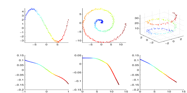
Fig. 1: sample data points with noise from various 1-D manifolds (top) and coordinates of computed $\tau_{i}$ via exact $\tau_{i}^{*}$ (bottom).

It is also important to better understand the failure modes of LTSA, and ultimately to identify conditions under which LTSA can truly uncover the hidden nonlinear structures of the data points. As we have shown in the error analysis in section 6, it will be difficult to align the local tangent information $\Theta_{i}$ if some of the $P_{i}$’s defined in (3.2) are close to be singular. One effect of this is that the computed coordinates $\tau_{i}$ and its neighbors may be compressed together. To clearly demonstrate this phenomenon, we consider the following function,

$$f(\tau)=[\cos^{3}(\tau),\,\,\sin^{3}(\tau)]^{T},\quad\tau\in[0,\,\pi].$$

The Jacobi matrix (now a single vector since $d=1$) given by

$$J_{f}(\tau)=1.5\sin(2\tau)[-\cos(\tau),\,\,\sin(\tau)]^{T}$$

is equal to zero at $\tau=\pi/2$. In that case the $\theta$-vector $\Theta_{i}$ defined in (4.5) will be computed poorly in the presence of noise. Usually the corresponding $\Theta_{i}$ will be small which also results in small $\tau_{i}$ and the neighbors of $\tau_{i}$ will also be small. In the first column of Fig 2, we plot the computed results for this 1-D curve. We see clearly near the singular point $\tau=\pi/2$ the computed $\tau_{i}$’s become very small, all compressed to a small interval around zero. In the second column of Fig 2, we examine another 1D curve defined by

$$f(\tau)=[10\cos(\tau),\,\,\sin(\tau)]^{T},\quad\tau\in[\pi/2,\,\,3\pi/2].$$

We notice that similar phenomenon also occurs near the point $\tau=\pi$ where the curvature of the curve is large, the computed $\tau_{i}$’s near the corresponding point also become very small, clustering around zero.

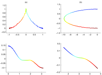
Fig. 2: 1-D manifolds with singular points (left) and corresponding coordinates $\tau_{i}$ via exact $\tau_{i}^{*}$ (right).

Next we look at the issues of the interaction of sampling density and noise levels. If there are large noises around $f(\tau_{i})$ relative to the sampling density near $f(\tau_{i})$, the resulting centered local data matrix $X_{i}(I-\frac{1}{k}ee^{T})$ will not be able to provide a good local tangent space, i.e., $X_{i}(I-\frac{1}{k}ee^{T})$ will have singular values $\sigma_{d}$ and $\sigma_{d+1}$ that are close to each other. This will result in a nearly singular matrix $P_{i}=Q_{i}^{T}J_{i}$, and when plotting $\tau_{i}^{*}$ against $\tau_{i}$, we will see the phenomenon of the computed coordinates $\tau_{i}$ getting compressed, similar to the case when the generating function $f(\tau)$ has singular and/or near-singular points. However, in this case, the result can usually be improved by increasing the number of neighbors used for producing the shifted matrix $X_{i}(I-\frac{1}{k}ee^{T})$. In Fig 3, we plot the computed results for the generating function

$$f(\tau)=3\tau^{3}+2\tau^{2}-2\tau,\quad\tau\in[-1.1,\,1].$$

The data set is generated by adding noise in a relative fashion,

$$x_{i}=f(\tau_{i})(1+\eta\epsilon_{i})$$

with normally distributed $\epsilon_{i}$. The first three columns in Fig 3 correspond to the noise levels $\eta=0.01$, $\eta=0.03$, and $\eta=0.05$, respectively. For the three data sets, We use the same number of neighbors, $k=10$. With the increasing noise level $\eta$, the computed $\tau_{i}$’s get expressed at points with relatively large noise. The quality of the computed $\tau_{i}$’s can be improved if we increase the number of neighbors as is shown on the column (d) in Fig 3. The improved result is for the same data set in column (c) with $k=20$ used.

Fig. 3: 1-D manifolds with different noise levels (top) and computed coordinates $\tau_{i}$ vs. exact $\tau_{i}^{*}$ (bottom).

As we have shown in Fig 3 (column (d)), different neighborhood size $k$ will produce different embedding results. In general, $k$ should be chosen to match the sampling density, noise level and the curvature at each data points so as to extract an accurate local tangent space. Too few neighbors used may result in a rank-deficient tangent space leading to over-fitting, while too large a neighborhood will introduce too much bias and the computed tangent space will not match the local geometry well. It is therefore worthy of considering variable number of neighbors that are adaptively chosen at each data point. Fortunately, our LTSA algorithm seems to be less sensitive to the choice of $k$ than LLE does as will be shown later.

We now apply LTSA to a $2$-D manifold embedded in a 100 dimensional space. The data points are generated as follows. First we generate $N=5000$ $3$D points,

$$x_{i}=(t_{i},\,s_{i},\,h(t_{i},s_{i}))^{T}+0.01\eta_{i}$$

with $t_{i}$ and $s_{i}$ uniformly distributed in the interval $[-1,\,\,1]$, the $\eta_{i}$’s are standard normal. The $h(t,s)$ is a peak function defined by

$$h(t,s)=0.3(1-t)^{2}e^{-t^{2}-(s+1)^{2}}-(0.2t-t^{3}-s^{5})e^{-t^{2}-s^{2}}-0.1e^{-(t+1)^{2}-s^{2}}.$$

This function is plotted in the left of Figure 4. We generate two kinds of data points $x_{i}^{Q}$ and $x_{i}^{H}$ in 100D space,

$$x_{i}^{Q}=Qx_{i},\quad x_{i}^{H}=Hx_{i},$$

where $Q$ is a random orthogonal matrix resulting in an orthogonal transformation and $H$ a matrix with its singular values uniformly distributed in $(0,\,1)$ resulting in an affine transformation. Figure 4 plots the coordinates for $x_{i}^{Q}$ (middle) and $x_{i}^{H}$ (right).

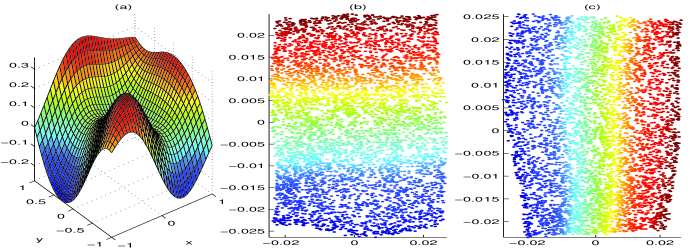
Fig. 4: 2-D manifold in a 100-D space generated by 3-D peak function: (a) 3-D peak curve, (b) coordinates for orthogonal transformed manifold, (c) coordinates for affine transformed manifold.

One advantage of LTSA over LLE is that using LTSA we can potentially detect the intrinsic dimension of the underlying manifold by analyzing the local tangent space structure. In particular, we can examine the distribution of the singular values of the local data matrix $X_{i}$ consisting of the data points in the neighborhood of each data point $x_{i}$. If the manifold is of dimension $d$, then $X_{i}$ will be close to a rank-$d$ matrix. We illustrate this point below. The data points are $x^{Q}_{i}$ of the $2$D peak manifold in the $100$D space. For each local data matrix $X_{i}$, let $\sigma_{j,i}$ be the $j$-the singular value of the centered matrix $X_{i}(I-\frac{1}{k}ee^{T})$. Define the ratios

$$\rho_{i}^{(j)}=\frac{\sigma_{j+1,i}}{\sigma_{j,i}}.$$

In Fig 5, we plot the rations $\rho_{i}^{(1)}$ and $\rho_{i}^{(2)}$. It clearly shows the feature space should be $2$-dimensional.

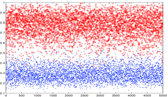
Fig. 5: Singular value ratios $\rho_{i}^{(1)}$ ($+$-dots) and $\rho_{i}^{(2)}$ ($\cdot$-dots).

Next, we discuss the issue of how to use the global coordinates $\tau_{i}$’s as a means for clustering the data points $x_{i}$’s. The situation is illustrated by Figure 6. The data set consists of three bivariate Gaussians with covariance matrices $0.2I_{2}$ and mean vectors located at $[1,1],[1,-1],[-1,0]$. There are $100$ sample points from each Gaussian. The thick curve on the right panel represents the principal curve computed by LTSA and the thin curve by LLE. It is seen that the thick curve goes through each of the Gaussians in turn, and the corresponding global coordinates (plotted in the middle panel) clearly separate the three Gaussians. LLE did not perform as well, mixing two of the Gaussians.

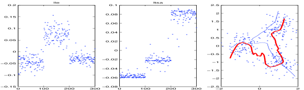
Fig. 6: (left) Global coordinates by LLE, (middle) global coordinates by LTSA, (right) Three Gaussian data with principal curves

Last we look at the results of applying LTSA algorithm to the face image data set [18]. The data set consists of a sequence $698$ $64$-by-$64$ pixel images of a face rendered under various pose and lighting conditions. Each image is converted to an $m=4096$ dimensional image vector. We apply LTSA with $k=12$ neighbors and $d=2$. The constructed coordinates are plotted in the middle of Figure 7. We also extracted four paths along the boundaries of of the set of the 2D coordinates, and display the corresponding images along each path. It can be seen that the computed 2D coordinates do capture very well the pose and lighting variations in a continuous way.

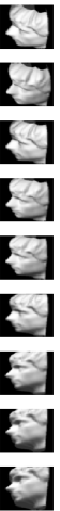
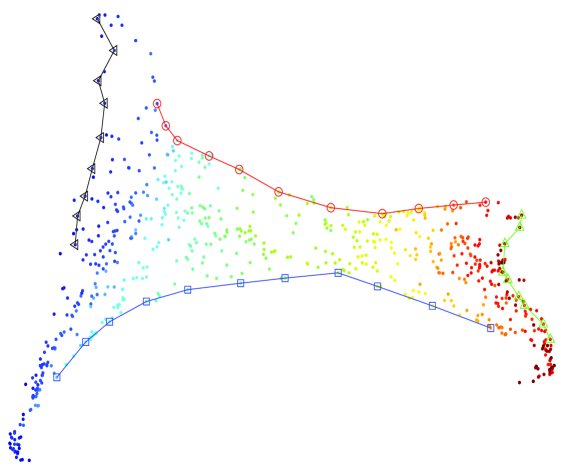
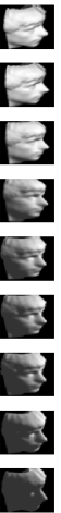
Fig. 7: Coordinates computed by Algorithm LTSA with $k=12$ neighbors (middle) and images corresponding to the points on the bound lines (top, bottom,left, and right) Left.

9 Conclusions and Feature Works

In this paper, we proposed a new algorithm (LTSA) for nonlinear manifold learning and nonlinear dimension reduction. The key techniques we used are construction of local tangent spaces to represent local geometry and the global alignment of the local tangent spaces to obtain the global coordinate system for the underlying manifold. We provide some careful error analysis to exhibit the interplay of approximation accuracy, sampling density, noise level and curvature structure of the manifold. In the following, we list several issues that deserve further investigation.

1. To make LTSA (similarly LLE) more robust against noise, we need to resolve the issue where several of the smallest eigenvalues of $B$ are about the same magnitude. This can be clearly seen when the manifold itself consists of several disjoint components. If this is the case, one needs to break the matrix $B$ into several diagonal blocks, and apply LTSA to each of the block. However, with noise, the situation becomes far more complicated, several eigenvectors corresponding to near-zero eigenvalues can mix together, the information of the global coordinates seems to be contained in the eigen-subspace, but how to unscramble the eigenvectors to extract the global coordinate information needs more careful analysis of the eigenvector matrix of $B$ and various models of the noise. Some preliminary results on this problem have been presented in [12].

2. The selection of the set of points to estimate the local tangent space is very crucial to the success of the algorithm. Ideally, we want this set of points to be close to the tangent space. However, with noise and/or at the points where the curvature of the manifold is large, this is not an easy task. One line of ideas is to do some preprocessing of the data points to construct some restricted local neighborhoods. For example, one can first compute the minimum Euclidean spanning tree for the data set, and restrict the neighbors of each point to those that are linked by the branches of the spanning tree. This idea has been applied in self-organizing map [10]. Another idea is to use iterative-refinement, combining the computed $\tau_{i}$’s with the $x_{i}$’s for neighborhood construction in another round of nonlinear projection. The rationale is that $\tau_{i}$’s as the computed global coordinates of the nonlinear manifold may give a better measure of the local geometry.

3. A discrete version of the manifold learning can be formulated by considering the data points as the vertices of an undirected graph [11]. A quantization of the global coordinates specifies the adjacency relation of those vertices, and manifold learning becomes discovering whether an edge should be created between a pair of vertices or not so that the resulting vertex neighbors resemble those of the manifold. We need to investigate a proper formulation of the problem and the related optimization methods.

4. From a statistical point of view, it is also of great interest to investigate more precise formulation of the error model and the associated consistency issues and convergence rate as the sample size goes to infinity. The learn-ability of the nonlinear manifold also depends on the sampling density of the data points. Some of the results in non-parametric regression and statistical learning theory will be helpful to pursue this line of research.

References

- [1] M. Belkin and P. Niyogi. Laplacian eigenmaps for dimension reduction and data representation. Technical Report, Dept. of Statistics, Univ. of Chicago, 2001.
- [2] D. Donoho and C. Grimes. When Does ISOMAP Recover the Natural Parametrization of Families of Articulated Images? Technical Report 2002-27, Department of Statistics, Stanford University, 2002.
- [3] D. Donoho and C. Grimes. Local ISOMAP perfectly recovers the underlying parametrization for families of occluded/lacunary images. To appear in IEEE Computer Vision & Pattern Recognition, 2003.
- [4] D. Freedman. Efficient simplicial reconstructions of manifolds from their samples. IEEE PAMI, to appear, 2002.
- [5] G. H. Golub and C. F. Van Loan. Matrix Computations. Johns Hopkins University Press, Baltimore, Maryland, 3nd edition, 1996.
- [6] T. Hastie and W. Stuetzle. Principal curves. J. Am. Statistical Assoc., 84: 502–516, 1988.
- [7] T. Hastie, R. Tibshirani and J. Friedman. The Elements of Statistical Learning. Springer, New York, 2001.
- [8] G. Hinton and S. Roweis. Stochastic Neighbor Embedding. To appear in Advances in Neural Information Processing Systems, 15, MIT Press (2003).
- [9] O. Jenkins and M. Mataric. Deriving action and behavior primitives from human motion data. Intl. Conf. on Robotics and Automation, 2002.
- [10] T. Kohonen. Self-organizing Maps. Springer-Verlag, 3rd Edition, 2000.
- [11] T. Martinetz and K. Schulten. Topology representing networks. Neural Networks, 7: 507–523, 1994.
- [12] M. Polito and P. Perona. Grouping and Dimensionality reduction by Locally Linear Embedding. Advances in Neural Information Processing Systems 14, eds. T. Dietterich, S. Becker, Z. Ghahramani, MIT Press (2002).
- [13] J.O. Ramsay and B.W. Silverman. Applied Functional Data Analysis. Springer, 2002.
- [14] S. Roweis and L. Saul. Nonlinear dimension reduction by locally linear embedding. Science, 290: 2323–2326, 2000.
- [15] S. Roweis and L. Saul and G. Hinton. Global coordination of local linear models Advances in Neural Information Processing Systems, 14:889–896, 2002.
- [16] L. Saul and S. Roweis. Think globally, fit locally: unsupervised learning of nonlinear manifolds. Technical Reports, MS CIS-02-18, Univ. Pennsylvania, 2002.
- [17] Y. Teh and S. Roweis. Automatic Alignment of Hidden Representations. To appear in Advances in Neural Information Processing Systems, 15, MIT Press (2003).
- [18] J. Tenenbaum, V. De Silva and J. Langford. A global geometric framework for nonlinear dimension reduction. Science, 290:2319–2323, 2000.
- [19] W.N. Venables and B.D. Ripley. Modern Applied Statistics with S-plus. Springer-verlag, 1999.