Survey propagation: an algorithm for satisfiability

Abstract

We study the satisfiability of randomly generated formulas formed by $M$ clauses of exactly $K$ literals over $N$ Boolean variables. For a given value of $N$ the problem is known to be most difficult when $\alpha=M/N$ is close to the experimental threshold $\alpha_{c}$ separating the region where almost all formulas are SAT from the region where all formulas are UNSAT. Recent results from a statistical physics analysis suggest that the difficulty is related to the existence of a clustering phenomenon of the solutions when $\alpha$ is close to (but smaller than) $\alpha_{c}$. We introduce a new type of message passing algorithm which allows to find efficiently a satisfiable assignment of the variables in this difficult region. This algorithm is iterative and composed of two main parts. The first is a message-passing procedure which generalizes the usual methods like Sum-Product or Belief Propagation: it passes messages that are surveys over clusters of the ordinary messages. The second part uses the detailed probabilistic information obtained from the surveys in order to fix variables and simplify the problem. Eventually, the simplified problem that remains is solved by a conventional heuristic.

I Introduction

The satisfiability problem is the archetype of combinatorial optimization problems which are well known to be intractable in the worst case. However, experimental studies show that many instances of satisfiability are surprisingly easy, even for naive heuristic algorithms. In an attempt to get a better understanding of which instances are easy or hard to solve, a lot of efforts have focused in recent years on the ’random K-sat’ problemCook_review . Instances of this problem are generated by considering $N$ variables and $M=\alpha N$ clauses, where each clause contains exactly $K$ distinct variables, and is picked up with uniform probability distribution from the set of $\left(\begin{array}[]{c}N\\ K\end{array}\right)2^{K}$ possible clauses. For a given value of $\alpha$, the probability $P_{N}(\alpha)$ that a randomly generated instance is SAT is a decreasing function, with $P_{N}(0)=1$ and $\lim_{\alpha\to\infty}P_{N}(\alpha=0)$, which has been shown to approach, as $N$ increases, a step function characteristic of a zero-one law friedgut , or a ‘phase transition’. It is convenient to identify a crossover regime between ’SAT’ and ’UNSAT’ regimes using the value $\alpha_{c}(N)$ of the number of constraints per variable where $P_{N}(\alpha_{c}(N))=1/2$. From numerical simulations, $\alpha_{c}(N)$ is supposed to converge, in the large $N$ limit, to a value around $\alpha_{c}\simeq 4.27$ TCS_issue ; KirkSel ; Crawford ; MZKST , but this convergence has not yet been established rigorously. Interestingly, the performance of algorithms is found to be much worse around this value of $\alpha=4.27$: randomly generated instances with $\alpha$ near to the phase transition are particularly difficult to solve.

Rigorous lower and upper bounds have been found for this conjectured satisfiability threshold: it has been established that $\lim_{N\to\infty}P_{N}(\alpha)=1$ for $\alpha<\alpha_{lb}$ and $\lim_{N\to\infty}P_{N}(\alpha)=0$ for $\alpha>\alpha_{ub}$. The present best bounds for the case of the random 3-SAT problem (with $K=3$) are $\alpha_{ub}=4.506$ (from dubois , using the first moment method) and $\alpha_{lb}=3.42$ (from Kirousis_lb , using algorithmic analysis). Note also the interesting algorithm-independent upper bound found in moore_achl ; achl_perez using the second moment method, which becomes better for larger values of $K$.

Recently, some elaborate statistical physics methods have been brought to bear on the random satisfiability problem. These non-rigorous analytical calculations have put forward some interesting conjectures about what happens in the solution space of the problem as this threshold is approachedMEPAZE ; MZ_pre (see also previous work in MonZec ; Biroli ). They suggest the following overall picture, which should hold for a generic sample of the random satisfiability problem, in the limit $N\to\infty$, with $\alpha$ fixed.

1. There exists a SAT-UNSAT phase transition at a critical value $\alpha_{c}$ which can be computed by solving some (complicated) integral equation; for $K=3$, one gets $\alpha_{c}\simeq 4.267$

2. There exists a second threshold $\alpha_{clust}$ separating two phases which are both ‘SAT’ (in each of them there exists a satisfiable assignment with probability 1), but with very different geometric structures:

3. For $\alpha<\alpha_{clust}$, a generic problem has many solutions, which tend to form one giant “cluster”; the set of all satisfying assignments forms a connected cluster in which it is possible to find a path between two solutions that requires short steps only (each pair of consecutive assignments in the path are close together in Hamming distance). In this regime, local search algorithms and other simple heuristics can relatively easily find a solution. This region is called the ’easy-SAT’ region

4. For $\alpha_{clust}<\alpha<\alpha_{c}$, there exists a ’hard SAT’ phase where the solution space breaks up into many smaller clusters. Solutions in separate clusters are generally far apart: it is not possible to transform a SAT assignment in one cluster into another one in a different cluster by changing only a finite number of variables. Because of this clustering effect, local search algorithms tend to have a very slow convergence when applied to large $N$ instances.

So far, the analytic method used in the most recent statistical physics analysis, named the cavity methodBethe_cav , is non rigorous, and turning this type of approach into a rigorous theory is an open subject of current researchtalag ; FraLeo . Note however that, in the simpler case of the random K-XOR-SAT, the validity of this statistical physics analysis can be confirmed by rigorous studies xorsat1 ; xorsat2 , and the above clustering conjecture has been fully confirmed.

Interestingly, the statistical physics analysis suggests a new efficient heuristic algorithm for finding SAT assignments in the hard SAT phase, which has been put forward by two of us in MZ_pre . The aim of this paper is to provide a detailed self-contained description of this algorithm, which does not rely on the statistical physics background. We shall limit the description to the regime where solutions exist, the so called SAT phase; some modification of the algorithm allows to address the optimization problem of minimizing the number of violated constraints in the UNSAT phase, but it will not be discussed here.

The basic building block of the algorithm, called survey propagation (SP), is a message passing procedure which resembles in some respect the iterative algorithm known as belief propagation (BP), but with some crucial differences which will be described. BP is a generic algorithm for computing marginal probability distributions in problems defined on factor graphs, which has been very useful in the context of error correcting codes Gallager and Bayesian networks pearl .

While in simple limits we are able to give some rigorous results together with an explicit comparison with the belief propagation procedures, in general there exists no rigorous proof of convergence of the algorithm. However, we provide clear numerical evidence of its performance over benchmarks problems which appear to be far larger than those which can be handled by present state-of-the-art algorithms.

The paper is organized as follows: Sect. II describes the satisfiability problem and its graphical representation in terms of a factor graph. Sect. III explains two message passing algorithms, namely warning propagation (WP) and belief propagation (BP). Both are exact for tree factor graphs. Even if they are typically unable to find a solution for random SAT in the “interesting” hard-SAT region, they are shown here because they are in some sense the basic building blocks of our survey propagation algorithm. Sect. IV explains the survey propagation algorithm itself, a decimation procedure based on it, the ‘survey inspired decimation’ (SID), and the numerical results. In Sect.V we give some heuristic arguments from statistical physics which may help the reader to understand where the SP algorithm comes from. Sect. VI contains a few general comments.

II The SAT problem and its factor graph representation

We consider a satisfiability problem consisting of $N$ Boolean variables $\{x_{i}\in\{0,1\}\}$ (where $\{0,1\}\equiv\{F,T\}$), with $i\in\{1,...,N\}$, with $M$ constraints. Each constraint is a clause, which is the logical OR of the variables or of their negations. A clause $a$ is characterized by the set of variables $i_{1},...,i_{K}$ which it contains, and the list of those which are negated, which can be characterized by a set of $K$ numbers $J^{a}_{i_{r}}\in\{\pm 1\}$ as follows. The clause is written as

$$\left(z_{i_{1}}\vee...\vee z_{i_{r}}\vee...\vee z_{i_{K}}\right)$$ (1)

where $z_{i_{r}}=x_{i_{r}}$ if $J^{a}_{i_{r}}=-1$ and $z_{i_{r}}=\bar{x}_{i_{r}}$ if $J^{a}_{i_{r}}=1$ (note that a positive literal is represented by a negative $J$). The problem is to find whether there exists an assignment of the $x_{i}\in\{0,1\}$ which is such that all the $M$ clauses are true. We define the total cost $C$ of a configuration ${\bf x}=(x_{1},...,x_{N})$ as the number of violated clauses.

In what follows we shall adopt the factor graph representation factor_graph of the SAT problem. This representation is convenient because it provides an easy graphical description to the message passing procedures which we shall develop. It also applies to a wide variety of different combinatorial problems, thereby providing a unified notation.

The SAT problem can be represented graphically as follows (see fig.1). Each of the $N$ variables is associated to a vertex in the graph, called a “variable node” (circles in the graphical representation), and each of the $M$ clauses is associated to another type of vertex in the graph, called a “function node” (squares in the graphical representation). A function node $a$ is connected to a variable node $i$ by an edge whenever the variable $x_{i}$ (or its negation) appears in the clause $a$. In the graphical representation, we use a full line between $a$ and $i$ whenever the variable appearing in the clause is $x_{i}$ (i.e. $J^{a}_{i}=-1$), a dashed line whenever the variable appearing in the clause is $\bar{x}_{i}$ (i.e. $J^{a}_{i}=1$). Variable nodes compose the set $X$ ($|X|=N$) and function nodes the set $A$ ($|A|=M$).

Figure 1: An example of a factor graph with $6$ variable nodes $i=1,..,6$ and $6$ function nodes $a,b,c,d,e,f$. The formula which is encoded is: $F=(x_{1}\vee\bar{x}_{3})\wedge(\bar{x}_{1}\vee x_{2}\vee x_{4})\wedge(\bar{x}_{3}\vee x_{5})\wedge(\bar{x}_{3}\vee\bar{x}_{4}\vee x_{5})\wedge(\bar{x}_{2}\vee x_{4}\vee x_{6})\wedge(x_{5})$

In summary, each SAT problem can be described by a bipartite graph, $G=\left(X\cup A;E=X\times A\right)$ where $E$ is the edge set, and by the set of “couplings” $\{J_{a}^{i}\}$ needed to define each function node. For the K-SAT problem where each clause contains $K$ variables, the degree of all the function nodes is $K$.

Throughout this paper, the variable nodes indices are taken in $i,j,k,...$, while the function nodes indices are taken in $a,b,c,...$. For every variable node $i$, we denote by $V(i)$ the set of function nodes $a$ to which it is connected by an edge, by $n_{i}=|V(i)|$ the degree of the node, by $V_{+}(i)$ the subset of $V(i)$ consisting of function nodes $a$ where the variable appears un-negated (the edge $(a,i)$ is a full line), and by $V_{-}(i)$ the complementary subset of $V(i)$ consisting of function nodes $a$ where the variable appears negated (the edge $(a,i)$ is a dashed line). $V(i)\setminus b$ denotes the set V(i) without a node $b$. Similarly, for each function node $a$, we denote by $V(a)=V_{+}(a)\cup V_{-}(a)$ the set of neighboring variable nodes, decomposed according to the type of edge connecting $a$ and $i$, and by $n_{a}$ the degree. Given a function node $a$ and a variable node $j$, connected by an edge, it is also convenient to define the two sets: $V^{u}_{a}(j)$ and $V^{s}_{a}(j)$, where the indices $s$ and $u$ respectively refer to the neighbors which tend to make variable $j$ satisfy or unsatisfy the clause $a$, defined as (see fig.2):

if $$J_{j}^{a}=1\;:\;\ V^{u}_{a}(j)=V_{+}(j)\ \ ;\ \ V^{s}_{a}(j)=V_{-}(j)\setminus a$$ (2)

if $$J_{j}^{a}=-1:\;\ V^{u}_{a}(j)=V_{-}(j)\ \ ;\ \ V^{s}_{a}(j)=V_{+}(j)\setminus a$$ (3)

Figure 2: A function node $a$ of the factor graph with the $V^{u}_{a}(j)$ and $V^{s}_{a}(j)$ sets relative to node $j$.

The same kind of factor graph representation can be used for other constraint satisfaction problems, where each function node $a$ defines an arbitrary function over the set $X_{a}\subset X$ of variable nodes to which is connected, and could also involve hidden variables.

III The message passing solution of SAT on a tree

In the special case in which the factor graph of a SAT problem is a tree (we shall call it a tree-problem), the satisfiability problem can be easily solved by many methods. Here we shall describe two message passing algorithms. The first one, called warning propagation (WP), determines whether a tree-problem is SAT or not; if it is SAT, WP finds one satisfiable assignment. The second algorithm, called belief propagation (BP), computes the number of satisfiable assignments, as well as the fraction of these assignments where a given variable is set to true. These algorithms are exact for tree-problems, but they can be used as heuristic in general problems, and we first give their general definition, which does not rely on the tree-like structure of the factor graph.

III.1 Warning propagation

The basic elementary message passed from one function node $a$ to a variable $i$ (connected by an edge) is a Boolean number $u_{a\to i}\in\{0,1\}$ called a ‘warning’.

The update rule is defined as follows. Given a function node $a$ and one of its variables nodes $i$, the warning $u_{a\to i}$ is determined from the warnings $u_{b\to j}$ arriving on all the variables $j\in V(a)\setminus i$ according to:

$$u_{a\to i}=\prod_{j\in V(a)\setminus i}\theta\left(-J^{a}_{j}\left(\sum_{b\in V(j)\setminus a}J^{b}_{j}u_{b\to j}\right)\right)\ ,$$ (4)

where $\theta(x)=0$ if $x\leq 0$ and $\theta(x)=1$ if $x>0$. This update rule is used sequentially, resulting in the following algorithm:

 
WP algorithm

INPUT: the factor graph of a Boolean formula in conjunctive normal form; a maximal number of iterations $t_{max}$

OUTPUT: UN-CONVERGED if WP has not converged after $t_{max}$ sweeps. If it has converged: the set of all warnings $u_{a\to i}^{*}$.

 

• At time $t=0$: For every edge $a\to i$ of the factor graph, randomly initialize the warnings $u_{a\to i}(t=0)\in\{0,1\}$, e.g. with probability $1/2$.

• For $t=1$ to $t=t_{max}$:

  • sweep the set of edges in a random order, and update sequentially the warnings on all the edges of the graph, generating the values $u_{a\to i}(t)$, using subroutine WP-UPDATE.

  • If $u_{a\to i}(t)=u_{a\to i}(t-1)$ on all the edges, the iteration has converged and generated $u_{a\to i}^{*}=u_{a\to i}(t)$: go to 2.

• If $t=t_{max}$ return UN-CONVERGED. If $t<t_{max}$ return the set of fixed point warnings $u_{a\to i}^{*}=u_{a\to i}(t)$

 

Subroutine WP-UPDATE$(u_{a\to i})$

INPUT: Set of all warnings arriving onto each variable node $j\in V(a)\setminus i$

OUTPUT: new value for the warning $u_{a\to i}$.

• For every $j\in V(a)\setminus i$, compute the cavity field $h_{j\to a}=\left(\sum_{b\in V_{+}(j)\setminus a}u_{b\to j}\right)-\left(\sum_{b\in V_{-}(j)\setminus a}u_{b\to j}\right)$ (If $V(j)\setminus a$ is empty, then $h_{j\to a}=0$).

• Using these cavity fields $h_{j\to a}$, compute the warning $u_{a\to i}=\prod_{j\in V(a)\setminus i}\theta\left(h_{j\to a}J^{a}_{j}\right)$ (If $V(a)\setminus i$ is empty, then $u_{a\to i}=1$).

 

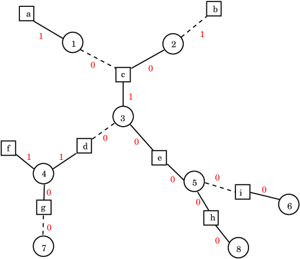
Figure 3: An example of result obtained by the WP algorithm on a tree-problem with $N=8$ variables and $M=9$ clauses. The number on each edge of the graph is the value of the corresponding warning $u^{*}$. The local fields on the variable are thus: $1,-1,1,2,0,0,0,0$. The satisfiable assignments are such that $x_{1}=1,x_{2}=0,x_{3}=1,x_{4}=1$, $x_{7}\in\{0,1\}$, $(x_{5},x_{6},x_{8})\in\{(1,1,1),(1,1,0),(0,1,1),(0,0,1)\}$. One can check that the variables with nonzero local field take the same value in all SAT assignments. In the WID algorithm, the variables $1,2,3,4$ are fixed to $x_{1}=1,x_{2}=0,x_{3}=1,x_{4}=1$; the remaining tree has only the clauses $h$ and $i$ remaining, and all the warnings are $u^{*}=0$. The variable $x_{7}$ will be fixed arbitrarily. If one chooses for instance $x_{5}=1$, the remaining graph leaves $x_{8}$ unconstrained but imposes $x_{6}=1$, as can be checked by applying to it the BP algorithm.

The interpretation of the messages and the message-passing procedure is the following. A warning $u_{a\to i}=1$ can be interpreted as a message sent from function node $a$, telling the variable $i$ that it should adopt the correct value in order to satisfy clause $a$. This is decided by $a$ according to the messages which it received from all the other variables $j$ to which it is connected: if $\left(\sum_{b\in V(j)\setminus a}J^{b}_{j}u_{b\to j}\right)J^{a}_{j}<0$, this means that the tendency for site $j$ (in the absence of $a$) would be to take a value which does not satisfy clause $a$. If all neighbors $j\in V(a)\setminus i$ are in this situation, then $a$ sends a warning to $i$. An example of the use of WP is shown in fig. 3.

The warning propagation algorithm can be applied to any SAT problem. When it converges, this dynamics defines a fixed point, which is a set of warnings $u_{a\to i}^{*}$. These can be used to compute, for each variable $i$, the “local field” $H_{i}$ and the “contradiction number” $c_{i}$ which are two integers defined as:

$$H_{i}=-\sum_{b\in V(i)}J^{b}_{i}u_{b\to i}^{*}$$ (5)

$$c_{i} = 1\ \ \ \ \mbox{if}\ \ \left(\sum_{b\in V_{+}(i)}u_{b\to i}^{*}\right)\left(\sum_{b\in V_{-}(i)}u_{b\to i}^{*}\right)>0$$ (6)

$$c_{i} = 0\ \ \ \ \mbox{otherwise.}$$ (7)

The local field $H_{i}$ is an indication of the preferred state of the variable $i$: $x_{i}=1$ if $H_{i}>0$, $x_{i}=0$ if $H_{i}<0$. The contradiction number indicates whether the variable i has received conflicting messages.

The interest in WP largely comes from the fact that it gives the exact solution for tree-problems. This is summarized in the following simple theorem:

THEOREM 1:

Consider an instance of the SAT problem for which the factor graph is a tree. Then the WP algorithm converges to a unique set of fixed point warnings $u_{a\to i}^{*}$, independently on the initial warnings. If at least one of the corresponding contradiction numbers $c_{i}$ is equal to $1$, the problem is UNSAT, otherwise it is SAT.

Corollary: In the case where the problem is SAT, the local fields $H_{i}$ can be used to find an assignment of the variables satisfying all the clauses, using the following algorithm called “Warning Inspired Decimation” or WID:  
WID algorithm INPUT: the factor graph of a Boolean formula in conjunctive normal form OUTPUT: UN-CONVERGED, or status of the formula (SAT or UNSAT); If the formula is SAT: one assignment which satisfies all clauses.   1. While the number of unfixed variables is $>0$, do: 1.1 Run WP 1.2 If WP does not converge, return UN-CONVERGED. Else compute the local fields $H_{i}$ and the contradiction numbers $c_{i}$, using eqs. (5,7). 1.3 If there is at least one contradiction number $c_{i}=1$, return UNSAT. Else: 1.3.1 If there is at least one local field $H_{i}\neq 0$: fix all variables with $H_{i}\neq 0$ ($H_{i}>0\Rightarrow x_{i}=1$ and $H_{i}<0\Rightarrow x_{i}=0$ ), and clean the graph, which means: $\{$ remove the clauses satisfied by this fixing, reduce the clauses that involve the fixed variable with opposite literal, update the number of unfixed variables$\}$. GOTO label 1. Else: 1.3.2 Choose one unfixed variable, fix it to an arbitrary value, clean the graph. GOTO label 1 2. return the set of assignments for all the variables.  

PROOF of theorem 1:

The convergence of message passing procedures on tree graphs is a well known result (see e.g.factor_graph ). We give here an elementary proof of convergence for the specific case of WP, and then show how the results on $H_{i}$ and $c_{i}$ follow.

Call ${\cal E}$ the set of nodes. Define the leaves of the tree, as the nodes of degree $1$. For any edge $(a,i)$ connecting a function node $a$ to a variable node $i$, define its level $r$ as follows: remove the edge $(a,i)$ and consider the remaining subgraph containing $a$. This subgraph ${\cal T}_{a-i}$ is a tree factor graph defining a new SAT problem. The level $r$ is the maximal distance between $a$ and all the leaves in the subgraph ${\cal T}_{(a,i)}$ (the distance between two nodes of the graph is the number of edges of the shortest path connecting them). If an edge $(a,i)$ has level $r=0$ (which means that $a$ is a leaf of the subgraph), $u_{a\to i}(t)=1$ for all $t\geq 1$. If $(a,i)$ has level $r=1$, then $u_{a\to i}(t)=0$ for all $t\geq 1$. From the iteration rule, a warning $u_{a\to i}$ at level $r$ is fully determined from the knowledge of all the warnings $u_{b\to j}$ at levels $\leq r-2$. Therefore the warning $u_{a\to i}(t)$ at a level $r$ is guaranteed to take a fixed value $u_{a\to i}^{*}$ for $t\geq 1+r/2$.

Let us now turn to the study of local fields and contradiction numbers.

We first prove the following lemma:

If a warning $u_{a\to i}^{*}=1$, the clause $a$ is violated in the reduced SAT problem defined by the subgraph ${\cal T}_{a\to i}$.

This is obviously true if the edge has level $r=0$ or $r=1$. Supposing that it holds for all levels $\leq r-2$, one considers an edge $a-i$ at level $r$, with $u_{a\to i}^{*}=1$. From (4), this means that for all variable nodes $j\in V(a)\setminus i$, the node $j$ receives at least one message from a neighboring factor node $b\in V(j)\setminus a$ with $u_{b\to j}=1$. The edge $b-j$ is at level $\leq r-2$, therefore the reduced problem on the graph ${\cal T}_{b-j}$ is UNSAT and therefore the clause $b$ imposes the value of the variable $j$ to be $1$ (True) if $J_{j}^{b}=-1$, or $0$ (False) if $J_{j}^{b}=1$: we shall say that clause $b$ fixes the value of variable $j$. This is true for all $j\in V(a)\setminus i$, which means that the reduced problem on ${\cal T}_{(a,i)}$ is UNSAT, or equivalently, the clause $a$ fixes the value of variable $i$.

Having shown that $u_{a\to i}^{*}=1$ implies that clause $a$ fixes the value of variable $i$, it is clear from (7) that a nonzero contradiction number $c_{i}$ implies that the formula is UNSAT.

If all the $c_{i}$ vanish, the formula is SAT. One can prove this for instance by showing that the WID algorithm generates a SAT assignment. The variables with $H_{i}\neq 0$ receive some nonzero $u_{a\to i}^{*}=1$ and are fixed. One then ’cleans’ the graph, which means: remove the clauses satisfied by this fixing, reduce the clauses that involve the fixed variable with opposite literal. By definition, this process has removed from the graph all the edges on which there was a nonzero warning. So on the new graph, all the edges have $u^{*}=0$. Following the step 2.2 of WID, one chooses randomly a variable $i$, one fixes it to an arbitrary value $x_{i}$, and cleans the graph. The clauses $a$ connected to $i$ which are satisfied by the choice $x_{i}$ are removed; the corresponding subgraphs are trees where all the edges have $u^{*}=0$. A clause $a$ connected to $i$ which are not satisfied by the choice $x_{i}$ may send some $u^{*}=1$ messages (this happens if such a clause had degree $2$ before fixing variable $i$). However, running WP on the corresponding subgraph ${\cal T}_{(a,i)}$, the set of warnings can not have a contradiction: A variable $j$ in this subgraph can receive at most one $u^{*}=1$ warning, coming from the unique path which connects $j$ to $a$. Therefore $c_{j}=0$: one iteration of WID has generated a strictly smaller graph with no contradiction. By induction, it thus finds a SAT assignment.$\square$

One should notice that the variables which are fixed at the first iteration of WID (those with non-zero $H_{i}$) are constrained to take the same value in all satisfiable assignments.

III.2 Belief propagation

While the WP algorithm is well adapted to finding a SAT assignment, the more complicated belief propagation (BP) algorithm is able to compute, for satisfiable problems with a tree factor graph, the total number of SAT assignments, and the fraction of SAT assignments where a given variable $x_{i}$ is true.

We consider a satisfiable instance, and the probability space built by all SAT assignments taken with equal probability. Calling $a$ one of the clauses in which $x_{i}$ appears, the basic ingredients of BP are the messages:

• $\mu_{a\to i}(x_{i})\in[0,1]$, interpreted as the probability that clause $a$ is satisfied, given the value of the variable $x_{i}\in\{0,1\}$.

• $\mu_{i\to a}(x_{i})\in[0,1]$, interpreted as the probability that the variable takes value $x_{i}$, when clause $a$ is absent (this is again a typical ’cavity’ definition). Notice that $\sum_{x_{i}\in\{0,1\}}\mu_{i\to a}(x_{i})=1$, while there is no such normalization for $\mu_{a\to i}(x_{i})$.

The BP equations are:

$$\mu_{i\to a}(x_{i})=C_{i\to a}\prod_{b\in V(i)\setminus a}\mu_{b\to i}(x_{i})\ ,$$ (8)

$$\mu_{a\to i}(x_{i})=\sum_{\{x_{j}(j\neq i)\}}f_{a}(X)\prod_{j\in V(a)\setminus i}\mu_{j\to a}(x_{j})\ ,$$ (9)

where $C_{i\to a}$ is a normalization constant ensuring that $\mu_{i\to a}$ is a probability, the sum over $\{x_{j}(j\neq i)\}$ means a sum over all values of the variables $x_{j}\in\{0,1\}$, for all $j$ different from $i$, and $f_{a}(X)$ is a characteristic function taking value $1$ if the configuration $X=\{x_{i}\}$ satisfies clause $a$, taking value $0$ otherwise.

It is convenient to parameterize $\mu_{i\to a}(x_{i})$ by introducing the number $\gamma_{i\to a}\in[0,1]$ which is the probability that the variable $x_{i}$ is in the state which violates clause $a$, in a problem where clause $a$ would be absent (writing for instance $\mu_{i\to a}(x_{i})=\gamma_{i\to a}\delta(x_{i},0)+(1-\gamma_{i\to a})\delta(x_{i},1)$ in the case where $J_{i}^{a}=-1$).

Let us denote by

$$\delta_{a\to i}\equiv\prod_{j\in V(a)\setminus i}\gamma_{j\to a}$$ (10)

the probability that all variables in clause $a$, except variable $i$, are in the state which violates the clause.

The BP algorithm amounts to an iterative update of the messages $\delta_{a\to i}$ according to the rule:

 
BP algorithm: INPUT: the factor graph of a Boolean formula in conjunctive normal form; a maximal number of iterations $t_{max}$; a requested precision $\epsilon$.

OUTPUT: UN-CONVERGED if BP has not converged after $t_{max}$ sweeps. If it has converged: the set of all messages $\delta_{a\to i}^{*}$.

 

• At time $t=0$: For every edge $a\to i$ of the factor graph, randomly initialize the messages $\delta_{a\to i}(t=0)\in[0,1]$

• For $t=1$ to $t=t_{max}$:

  • sweep the set of edges in a random order, and update sequentially the warnings on all the edges of the graph, generating the values $\delta_{a\to i}(t)$, using subroutine BP-UPDATE.

  • If $|\delta_{a\to i}(t)-\delta_{a\to i}(t-1)|<\epsilon$ on all the edges, the iteration has converged and generated $\delta_{a\to i}^{*}=\delta_{a\to i}(t)$: go to 2.

• If $t=t_{max}$ return UN-CONVERGED. If $t<t_{max}$ return the set of fixed point warnings $\delta{a\to i}^{*}=\delta_{a\to i}(t)$

 

 
Subroutine BP-UPDATE$(\delta_{a\to i})$

INPUT: Set of all messages arriving onto each variable node $j\in V(a)\setminus i$

OUTPUT: new value for the message $\delta_{a\to i}$.

 

• For every $j\in V(a)\setminus i$, compute the cavity field

  $$\gamma_{j\to a}=\frac{P^{u}_{j\to a}}{P^{u}_{j\to a}+P^{s}_{j\to a}}$$ (11)

  where

  $$P^{u}_{j\to a} = \prod_{b\in V_{a}^{s}(j)}(1-\delta_{b\to j})\ ,$$

  $$P^{s}_{j\to a} = \prod_{b\in V_{a}^{u}(j)}(1-\delta_{b\to j})\ .$$ (12)

  If an ensemble is empty, for instance $V_{a}^{s}(j)=\emptyset$, the corresponding $P^{u}_{j\to a}$ takes value $1$ by definition.

• Using these numbers $\gamma_{j\to a}$, compute the new message: $\delta_{a\to i}\equiv\prod_{j\in V(a)\setminus i}\gamma_{j\to a}$. If a factor node $a$ is a leaf (unit clause) with a single neighbor $i$, the corresponding $\delta_{a\to i}$ takes value $1$ by definition.

 

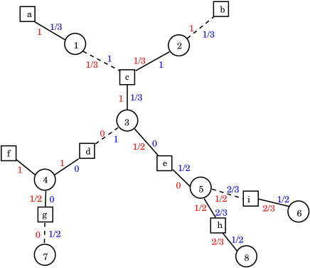
Figure 4: An example of result obtained by the BP algorithm on the tree-problem with $N=8$ variables and $M=9$ clauses studied in fig.3. On each edge of the graph connecting a function node like $c$ to a variable node like $2$, appears the value of $\gamma_{2\to c}$ (in blue, on the right hand side of the edge) and of $\delta_{c\to 2}$ (in red, on the left hand side of the edge). Comparing to the WP result of fig.3, one sees that all the messages $\delta_{a\to i}=1$, corresponding to strict warnings, are the same, while the messages $\delta_{a\to i}<1$ are interpreted in WP as “no warning” (i.e. a null message). Using (13), the probability $\mu_{i}$ that each variable $x_{i}=1$ are found equal to: $1,0,1,1,1/2,3/4,3/4,1/2$. These are the exact results as can be checked by considering all satisfiable assignments as in fig.3.

As WP, the BP algorithm is exact on trees (see for instance factor_graph ). In fact it gives a more accurate results than WP since it allows to compute the exact probabilities $\mu_{i}$ (while WP identifies the variables which are fully constrained, and gives a zero local field on the other variables). A working example of BP is shown in fig.4. In this example and more in general for trees, BP also provides the exact number ${\cal N}$ of SAT assignments, as given by the following theorem:

THEOREM 2: Consider an instance of the SAT problem for which the factor graph is a tree, and there exist some SAT assignments. Then:

a) The BP algorithm converges to a unique set of fixed point messages $\delta^{*}_{a\to i}$.

b)The probability $\mu_{i}$ that the variable $x_{i}=1$ is given by:

$$\mu_{i}=\frac{\prod_{a\in V_{-}(i)}(1-\delta^{*}_{a\to i})}{\prod_{a\in V_{-}(i)}(1-\delta^{*}_{a\to i})+\prod_{a\in V_{+}(i)}(1-\delta^{*}_{a\to i})}\ .$$ (13)

c) The number of SAT assignments is ${\cal N}=\exp(S)$, where the entropy $S$ is given by:

$$S = \sum_{a\in A}\ln\left[\prod_{i\in V(a)}\left(\prod_{b\in V_{a}^{s}(i)}(1-\delta_{b\to i}^{*})+\prod_{b\in V_{a}^{u}(i)}(1-\delta_{b\to i}^{*})\right)-\prod_{i\in V(a)}\left(\prod_{b\in V_{a}^{u}(i)}(1-\delta_{b\to i}^{*})\right)\right]$$ (14)

$$+\sum_{i\in X}(1-n_{i})\ln\left[\prod_{b\in V_{+}(i)}(1-\delta_{b\to i}^{*})+\prod_{b\in V_{-}(i)}(1-\delta_{b\to i}^{*})\right]$$

PROOF:

The proof of convergence is simple, using the same strategy as the proof in sect.III: messages at level 0 and 1 are fixed automatically, and a message at level $r$ is fixed by the values of messages at lower levels.

The probability $\mu_{i}$ is computed from the same procedure as the one giving the BP equations (8,9), with the difference that one takes into account all neighbors of the site $i$.

The slightly more involved result is the one concerning the entropy. We use the probability measure $P(X)$ on the space of all assignments which has uniform probability for all SAT assignments and zero probability for all the assignments which violate at least one clause:

$$P(X)=\frac{1}{\cal N}\prod_{a\in A}f_{a}(X)\ .$$ (15)

From $P$ one can define the following marginals:

• the ’site marginal’ $p_{i}(x_{i})$ is the probability that variable $i$ takes value $x_{i}\in\{0,1\}$

• the ’clause marginal’ $p_{a}(X_{a})$ is the probability that the set of variables $x_{i},i\in V(a)$, takes a given value, denoted by $X_{a}$ (among the $2^{n_{a}}$ possible values).

For a tree factor graph, one easily shows by induction on the size of the graph that the full probability can be expressed in terms of the site and clause marginals as:

$$P(X)=\prod_{a\in A}p_{a}(X_{a})\prod_{i\in X}p_{i}(x_{i})^{1-n_{i}}\ .$$ (16)

The entropy $S=\ln({\cal N})$ is then obtained as

$$S=-\sum_{X}P(X)\ln P(X)=-\sum_{a}\sum_{X_{a}}p_{a}(X_{a})\ln[p_{a}(X_{a})]-\sum_{i}(1-n_{i})\sum_{x_{i}}p_{i}(x_{i})\ln[p_{i}(x_{i})]$$ (17)

Let us now derive the expression of this quantity in terms of the messages used in BP. One has:

$$p_{i}(x_{i})=c_{i}\prod_{b\in V(i)}\mu_{b\to i}(x_{i})$$ (18)

and

$$p_{a}(X_{a})=c_{a}f_{a}(X_{a})\prod_{i\in V(a)}\mu_{i\to a}(x_{i})\ ,$$ (19)

where $c_{i}$ and $c_{a}$ are two normalization constants. From (18) one gets after some reshuffling:

$$\sum_{i}(n_{i}-1)\sum_{x_{i}}p_{i}(x_{i})\ln p_{i}(x_{i})=\sum_{i}(n_{i}-1)\ln c_{i}+\sum_{a}\sum_{i\in V(a)}\sum_{X_{a}}p_{a}(X_{a})\ln\left[\prod_{b\in V(i)\setminus a}\mu_{b\to i}(x_{i})\right]\ ;$$ (20)

Using the BP equation (8), this gives:

$$\sum_{i}(n_{i}-1)\sum_{x_{i}}p_{i}(x_{i})\ln p_{i}(x_{i})=\sum_{i}(n_{i}-1)\ln c_{i}+\sum_{a}\sum_{X_{a}}p_{a}(X_{a})\ln\left[\prod_{i\in V(a)}\mu_{i\to a}(x_{i})f_{a}(X_{a})\right]-\sum_{a}\sum_{i\in V(a)}\ln C_{i\to a}\ ,$$ (21)

where the term $f_{a}(X_{a})$ inside the logarithm has been added, taking into account the fact that, as $f_{a}(X_{a})\in\{0,1\}$, one always has $p_{a}(X_{a})\ln f_{a}(X_{a})=0$. Therefore:

$$S=-\sum_{a}\ln c_{a}+\sum_{i}(n_{i}-1)\ln c_{i}-\sum_{a}\sum_{i\in V(a)}\ln C_{i\to a}$$ (22)

In the notations of (12), one has

$$c_{a}=\frac{1}{1-\prod_{i\in V(a)}\gamma_{i\to a}}=\frac{1}{1-\prod_{i\in V(a)}P^{u}_{i\to a}/(P^{u}_{i\to a}+P^{s}_{i\to a})}\ ,$$ (23)

$$C_{i\to a}=\frac{1}{P^{u}_{i\to a}+P^{s}_{i\to a}}\ ,$$ (24)

and

$$c_{i}=\frac{1}{\prod_{b\in V_{+}(i)}(1-\delta_{b\to i})+\prod_{b\in V_{-}(i)}(1-\delta_{b\to i})}\ .$$ (25)

Substitution into (22) gives the expression (14) for the entropy. $\square$

IV Survey Propagation

IV.1 The algorithm

The WP and BP algorithms have been shown to work for satisfiability problems where the factor graph is a tree. In more general cases where the factor graph has loops, they can be tried as heuristics, but there is no guarantee of convergence. In this section we present a new message passing algorithm, survey propagation (SP), which is also a heuristic, without any guarantee of convergence. It reduces to WP for tree-problems, but it turns out to be more efficient than WP or BP in experimental studies of random satisfiability problems. SP has been discovered using concepts developed in statistical physics under the name of ’cavity method’. Here we shall first present SP, then give some experimental results, and in the end expose the qualitative physical reasoning behind it.

A message of SP, called a survey, passed from one function node $a$ to a variable $i$ (connected by an edge) is a real number $\eta_{a\to i}\in[0,1]$. The SP algorithm uses exactly the same main procedure as BP (see III.2), but instead of calling the BP-UPDATE, it uses a different update rule, SP-UPDATE, defined as:

 
Subroutine SP-UPDATE$(\eta_{a\to i})$

INPUT: Set of all messages arriving onto each variable node $j\in V(a)\setminus i$

OUTPUT: new value for the message $\eta_{a\to i}$.

 

• For every $j\in V(a)\setminus i$, compute the three numbers:

  $$\Pi^{u}_{j\to a} = \left[1-\prod_{b\in V^{u}_{a}(j)}\left(1-\eta_{b\to j}\right)\right]\prod_{b\in V^{s}_{a}(j)}\left(1-\eta_{b\to j}\right)$$

  $$\Pi^{s}_{j\to a} = \left[1-\prod_{b\in V^{s}_{a}(j)}\left(1-\eta_{b\to j}\right)\right]\prod_{b\in V^{u}_{a}(j)}\left(1-\eta_{b\to j}\right)$$

  $$\Pi^{0}_{j\to a} = \prod_{b\in V(j)\setminus a}\left(1-\eta_{b\to j}\right)$$ (26)

  if a set like $V^{s}_{a}(j)$ is empty, the corresponding product takes value $1$ by definition.

• Using these numbers , compute and return the new survey:

  $$\eta_{a\to i}=\prod_{j\in V(a)\setminus i}\left[\frac{\Pi^{u}_{j\to a}}{\Pi^{u}_{j\to a}+\Pi^{s}_{j\to a}+\Pi^{0}_{j\to a}}\right]\ .$$ (27)

  If $V(a)\setminus i$ is empty, then $\eta_{a\to i}=1$.

 

Qualitatively, the statistical physics interpretation of the survey $\eta_{a\to i}$ is a probability that a warning is sent from $a$ to $i$ (see section V for details). Therefore, whenever the SP algorithm converges to a fixed-point set of messages $\eta_{a\to i}^{*}$, one can use it in a decimation procedure in order to find a satisfiable assignment, if such an assignment exists. This procedure, called the survey inspired decimation (SID), is a generalization of the WID algorithm III.1, defined by:

 

SID algorithm

INPUT: The factor graph of a Boolean formula in conjunctive normal form. A maximal number of iterations $t_{max}$ and a precision $\epsilon$ used in SP

OUTPUT: One assignment which satisfies all clauses, or ’SP UNCONVERGED’, or ’probably UNSAT’  

• Random initial condition for the surveys

• Run SP. If SP does not converge, return ’SP UNCONVERGED’ and stop (or restart, i.e.go to 0.). If SP converges, use the fixed-point surveys $\eta^{*}_{a\to i}$ in order to:

• Decimate:

  • If non-trivial surveys ($\{\eta\neq 0\}$) are found, then:

    • Evaluate, for each variable node $i$, the three ’biases’ $\{W_{i}^{(+)},W_{i}^{(-)},W_{i}^{(0)}\}$defined by:

      $$W_{i}^{(+)} = \frac{\hat{\Pi}_{i}^{+}}{\hat{\Pi}^{+}_{i}+\hat{\Pi}^{-}_{i}+\hat{\Pi}^{0}_{i}}$$ (28)

      $$W_{i}^{(-)} = \frac{\hat{\Pi}_{i}^{-}}{\hat{\Pi}^{+}_{i}+\hat{\Pi}^{-}_{i}+\hat{\Pi}^{0}_{i}}$$ (29)

      $$W_{i}^{(0)} = 1-W_{i}^{(+)}-W_{i}^{(-)}$$ (30)

      where $\hat{\Pi}_{i}^{+},\hat{\Pi}_{i}^{-},\hat{\Pi}_{i}^{0}$ are defined by

      $$\hat{\Pi}^{+}_{i} = \left[1-\prod_{a\in V_{+}(i)}\left(1-\eta^{*}_{a\to i}\right)\right]\prod_{a\in V_{-}(i)}\left(1-\eta^{*}_{a\to i}\right)$$

      $$\hat{\Pi}^{-}_{i} = \left[1-\prod_{a\in V_{-}(i)}\left(1-\eta^{*}_{a\to i}\right)\right]\prod_{a\in V_{+}(i)}\left(1-\eta^{*}_{a\to i}\right)$$

      $$\hat{\Pi}^{0}_{i} = \prod_{a\in V(i)}\left(1-\eta^{*}_{a\to i}\right)$$ (31)

    • fix the variable with the largest $|W_{i}^{(+)}-W_{i}^{(-)}|$ to the value $x_{i}=1$ if $W_{i}^{(+)}>W_{i}^{(-)}$, to the value $x_{i}=0$ if $W_{i}^{(+)}<W_{i}^{(-)}$. Clean the graph, which means: $\{$ remove the clauses satisfied by this fixing, reduce the clauses that involve the fixed variable with opposite literal, update the number of unfixed variables$\}$.

  • If all surveys are trivial ($\{\eta=0\}$) , then output the simplified sub-formula and run on it a local search process (e.g. walksat).

• If the problem is solved completely by unit clause propagation, then output “SAT” and stop. If no contradiction is found then continue the decimation process on the smaller problem (go to 1.) else (if a contradiction is reached) stop.

 

There exist several variants of this algorithm. In the code which is available at web , for performance reasons we update simultaneously all $\eta$ belonging to the same clause. The clauses to be updated are chosen in a random permutation order at each iteration step. The algorithm can also be randomized by fixing, instead of the most biased variables, one variable randomly chosen in the set of the x percent variables with the largest bias. This strategy allows to use some restart in the case where the algorithm has not found a solution. A fastest decimation can also be obtained by fixing in the step 2.1(b), instead of one variable, a fraction $f$ of the $N_{t}$ variables which have not yet been fixed (going back to $1$ variable when $fN_{t}<1$).

IV.2 Experimental study of the SP algorithm

In order to get some concrete information on the behaviour of SP for large but finite $N$, we have experimented SP and SID on single instances of the random 3-SAT problem with many variables, up to $N\sim 10^{7}$. In this section we summarize these (single machine) experiments and their results.

Instances of the 3-SAT problem were generated with the pseudo random number generator "Algorithm B" on p.32 of Knuth Knuth . However we found that results are stable with respect to changes in the random number generators. Formulas are generated by choosing k-tuples of variable indices at random (with no repetitions) and by negating variables with probability $0.5$.

We first discuss the behaviour of the SP algorithm itself. We have used a precision parameter $\epsilon=10^{-3}$ (smaller values don’t seem to increase performance significantly). Depending on the range of $\alpha$, we have found the following behaviours, for large enough $N$:

• For $\alpha<\alpha_{d}\sim 3.9$, SP converges towards the set of trivial messages $\eta_{a\to i}=0$, for all $a-i$ edges. All variables are under-constrained.

• For $3.9<\alpha<4.3$, SP converges to a unique fixed-point set of non-trivial messages, independently from the initial conditions, where a large fraction of the messages $\eta_{a\to i}$ are in $]0,1[$.

Notice that, for ‘small’ values of $N$, around $N=1000$, one often finds some instances in which SP does not converge. But the probability of convergence, at a given $\alpha<4.3$, increases with $N$. This is exemplified by the following quantitative measure of the performance of the SID algorithm (which uses SP). We have solved several instances of the random 3-SAT problem, for various values of $\alpha$ and $N$, using the SID algorithm in which we fix at each step the fraction $fN_{t}$ of variables with largest $\left|W_{i}^{(+)}-W_{i}^{(-)}\right|$. Table 5 gives in each case the fraction of samples which are solved by SID, in a single run of decimation (without any restart). The algorithm fails when, either SP does not converge, or the simplified sub-formula found by SID is not solved by walksat. The performance of SID improves when $N$ increases and when $f$ decreases. Notice that for $N=10^{5}$ we solve all the $50$ randomly generated instances at $\alpha=4.24$. For larger values of $\alpha$ the algorithm often fails. Notice that in such cases it does not give any information on whether the instance is UNSAT. Some failures may be due to UNSAT instances, others are just real failures of the SID for SAT instances. Few experiments on even larger instances ($N=10^{6},10^{7}$) have also been succesfully run (the limiting factor being the available computer memory needed to store formulas).

$N=$	$2.5\cdot 10^{4}$				$5.0\cdot 10^{4}$				$1.0\cdot 10^{5}$
$f$ \ $\alpha$	4.21	4.22	4.23	4.24	4.21	4.22	4.23	4.24	4.21	4.22	4.23	4.24
4%	86%	66%	28%	8%	98%	84%	52%	22%	100%	100%	72%	22%
2%	100%	86%	50%	22%	100%	98%	86%	48%			100%	68%
1%		94%	78%	32%		100%	94%	64%				88%
0.5%		98%	88%	50%			98%	66%				92%
0.25%		100%	90%	60%			100%	78%				92%
0.125%			94%	60%				84%				100%
$<t>$	1369	2428	4635	7843	1238	1751	3411	8607	1204	1557	2573	7461

Figure 5: Results obtained by solving with a single decimation run of the SID algorithm 50 random instances of 3-SAT with $N=25000,50000,100000$ and $\alpha=4.21,4.22,4.23,4.24$. SID was used by fixing variables in blocks $fN_{t}$, where $N_{t}$ is the number of unfixed variables at time $t$, and various runs used different values of $f$ taken in the geometric progression $f=4\%,2\%,1\%,.5\%,.25\%,.125\%$, stopping if the formula was solved. For each value of $(N,\alpha,f)$, we give the fraction of the 50 instances which were solved (i.e. for which the algorithm found a SAT assignement). The maximal number of iteration was taken equal to $10^{3}$ and the precision for convergence was taken equal to $10^{-3}$. The last row shows the number of complete iterations of SP averaged over the successful runs.

As shown by the data on the average total number of SP iterations along the successful solution process in table 5, the convergence time of the SP algorithm basically does not grow with $N$ (a growth like $\log N$, which could be expected from the geometrical properties of the factor graph, is not excluded). Therefore the process of computing all the SP messages $\eta^{*}_{a\to i}$ takes $\Theta(N)$, or maybe $\Theta(N\ln N)$, operations. If SID fixes at each step only one variable, it will thus converge in $\Theta(N^{2}\log N)$ operations (the time taken by walksat to solve the simplified sub-formula seems to grow more slowly). When we fix a fraction of variables at a time, we get a further reduction of the cost to $O(N(\ln N)^{2})$ (the second $\ln$ comes from sorting the biases).

A very basic yet complete version of the code which is intended to serve only for the study on random 3-SAT instances is available at the web site web . Generalization of the algorithm to other problems require some changes which are not implemented in the distributed code.

V Heuristic arguments

Survey propagation has been invented using powerful concepts and methods developed in the statistical physics of disordered systems, notably the cavity method for diluted problems Bethe_cav . In this section we want to give some short background on these methods, in order to help the reader understand where SP comes from, and maybe develop similar algorithms in other contexts. Unfortunately so far there is no rigorous derivation of the cavity method, so this whole section only contains heuristic arguments.

V.1 The physical picture underlying the SP construction: clustering of configurations

Let us start with a discussion of the validity of BP. As we saw in sect.III, BP aims at computing the marginal probability distribution of a variable $x_{i}$, within the probability space built by all SAT assignments, each being given equal probability. The message $\mu_{a\to i}(x_{i})$ used in BP can be computed exactly if one knows the joint probability distribution $P^{(a)}(X)$ of the variables in $X=\{x_{j},\;j\in V(a)\setminus i\}$, in the graph where clause $a$ is absent. Using the same notations as in (9), one has:

$$\mu_{a\to i}(x_{i})=\sum_{\{x_{j}(j\neq i)\}}f_{a}(X)P^{(a)}(X)$$ (32)

Comparing this eq. (32) to the eqs. (8,9) of BP, one sees that BP uses an approximation, namely the fact that the joint probability $P^{(a)}(X)$ factorizes: $P^{(a)}(X)\simeq\prod_{j\in V(a)\setminus i}\mu_{j\to a}(x_{j})$. This amounts to assuming that the variables $x_{j}$, for $j\in V(a)\setminus i$, are uncorrelated in the absence of clause $a$. This assumption is obviously correct when the factor graph is a tree, which confirms the validity of BP in that case. In a general problem, for such an assumption to hold, we need two conditions to be fulfilled:

• the variables $x_{j},j\in V(a)\setminus i$ should be far from each other, in the factor graph where clause $a$ is absent.

• there should be a single phase in the problem, or the probability measure should be reduced to one single pure phase.

The first condition is easily understood, and one can see that it is generically fulfilled when one considers a random satisfiability problem. In random K-sat with $M=\alpha N$ clauses, the factor graph is a random bipartite graph, where function nodes have degree $K$ and variable nodes have fluctuating degrees, with a distribution which becomes, in the large $N$ limit, a Poisson law of mean $K\alpha$. Locally such a graph is tree like. Taking a clause $a$ at random, the minimal distance between two of the variables $x_{j},j\in V(a)\setminus i$ is generically of order $\log N$.

The second condition is more subtle. In general a pure phase is defined in statistical physics as an extremal Gibbs measure georgii ; however the standard construction of Gibbs measures deals with infinite systems. Here we need to work with $N$ variables where $N\gg 1$ but is finite, and the corresponding construction has not been worked out yet. For the random satisfiability problem, a heuristic description of a pure phase is a cluster of SAT assignments, defined as follows. Consider all SAT assignments. Define the distance between two assignments $\{x_{i}\}$ and $\{y_{i}\}$ as $\sum_{i}(x_{i}-y_{i})^{2}$. If the distance between two SAT assignment is smaller than a number $q$, they are said to belong to the same $q$-cluster. This allows to partition the set of SAT assignments into $q$-clusters. One is interested in the ’clusters’ obtained in large $N$ – large $q$ limit of the $q$-clusters, where the large $N$ limit is taken first. Heuristic statistical physics arguments indicate that, in the random K-satisfiability problem, for $\alpha<\alpha_{clust}(K)$, there should exist one single such cluster of SAT assignments: this means that one can move inside the space of SAT assignment, from any assignment to another one, by a succession of moves involving each a number of flips of variables which is $<<N$. In such a case the BP factorization approximation is expected to be correct. On the other hand, for $\alpha>\alpha_{clust}(K)$ the space of SAT assignment separates into many distant clusters, and the BP factorization does not hold globally, but it would hold if one could restrict the probability space to one given cluster $\alpha$. Within such a restricted space, BP would converge to a set of messages $\mu_{a\to i}^{\alpha}(x_{i})$ which depends on the cluster $\alpha$.

In this situation, the cavity method uses a statistical approach. It considers all the clusters of SAT assignments, and attributes to each cluster a probability proportional to the number of configuration that it contains. Then one introduces, on each edge $a-i$, a survey which gives the probability, when a cluster $\alpha$ is chosen randomly with this probability, that the message $\mu_{a\to i}^{\alpha}(x)$ is equal to a certain function $P(x)$.

This object is a probability of a probability and it is thus difficult to use in practical algorithms. For this reason, SP departs from the usual cavity method and uses a simpler object which is a survey of warnings, interpreted as follows: Consider one cluster $\alpha$ and an edge $a-i$ of the factor graph. If, in every SAT assignments of the cluster $\alpha$, all the variables $x_{j},j\in V(a)\setminus i$ don’t satisfy clause $a$, then a warning $u_{a\to i}^{\alpha}=1$ is passed along the edge from $a$ to $i$. The SP message along this edge is the survey of these warnings, when one picks up a cluster $\alpha$ at random: $\eta_{a\to i}=\sum_{\alpha}u_{a\to i}^{\alpha}/(\sum_{\alpha}1)$. So basically the SP message gives the probability that there is a warning sent from $a$ to $i$ in a randomly chosen cluster. With respect to the full-fledged cavity method, this is a much simplified object, which focuses onto the variables which are constrained.

The experimental results on random 3-satisfiability discussed in sect. IV.2 confirm the theoretical analysis of MEPAZE ; MZ_pre which indicate that all $\eta_{a\to i}$ vanish for $\alpha<\alpha_{d}\simeq 3.91$. This can be interpreted as the fact that, in this range of $\alpha$, there are no ’constrained clusters’ (meaning clusters in which some of the variables are constrained). For $\alpha_{d}<\alpha<\alpha_{c}=4.267$ the theory predicts the existence of non-trivial messages, meaning that there exist constrained clusters. This is the region where SP and SID are able to outperform existing algorithms. One should notice that the SID does not seem to converge up to the conjectured threshold $\alpha_{c}=4.267$: although it is very small, there remains a region in the ’Hard SAT’ phase, close to $\alpha_{c}$ where the simple version of SP/SID does not give the result. Recent work shows that this gap can be reduced by using some backtracking strategy in SIDParisi_backtrack . Whether it will be possible to close the gap with generalized versions of SP/SID, while keeping a typically polynomial running time, is an interesting open issue.

V.2 The “don’t-care” state

In a given cluster $\alpha$, a variable $x_{i}$ can be thought of being in three possible states: either it is constrained equal to $0$ (this means that $x_{i}=0$ in all SAT assignments of the cluster $\alpha$), or it is constrained equal to $1$, or it is not constrained. In this last situation we attribute it the value $*$. Therefore we can describe a cluster by the values of the $N$ generalized variables $x_{i}^{\alpha}\in\{0,1,*\}$, where $*$ will be denoted as the don’t-care state. Such a description associates to each cluster a single point in $\{0,1,*\}^{N}$. It discards a lot of information: $x_{i}^{\alpha}=*$ has lost all the information on the fraction of assignments in the cluster $\alpha$ where $x_{i}=0$. But it gives a simplified description of the cluster and it focuses onto the constrained variables.

It is interesting to notice that the SP equations can be interpreted as BP equations in the presence of this extra don’t-care state. This can be seen as follows. Borrowing the notations of the BP equations (8, 9) we denote by $\gamma_{i\to a}\in[0,1]$ the probability that the variable $x_{i}$ is in the state which violates clause $a$, in a problem where clause $a$ would be absent, and by

$$\delta_{a\to i}=\prod_{j\in V(a)\setminus i}\gamma_{j\to a}$$ (33)

the probability that all variables in clause $a$, except variable $i$, are in the state which violates the clause.

Let us compute $\mu_{i\to a}(x_{i})$. This depends on the messages sent from the nodes $b\in\{V(i)\setminus a\}$ to variable $i$. The various possibilities for these messages are:

• No warning arriving from $b\in V_{a}^{s}(i)$, and no warning arriving from $b\in V_{a}^{u}(i)$. This happens with a probability

  $$\Pi^{0}_{i\to a}=\prod_{b\in V(i)\setminus a}\left(1-\delta_{b\to i}\right)$$ (34)

• No warning arriving from $b\in V_{a}^{s}(i)$, and at least one warning arriving from $b\in V_{a}^{u}(i)$. This happens with a probability

  $$\Pi^{u}_{i\to a}=\left[1-\prod_{b\in V^{u}_{a}(i)}\left(1-\delta_{b\to i}\right)\right]\prod_{b\in V^{s}_{a}(i)}\left(1-\delta_{b\to i}\right)$$ (35)

• No warning arriving from $b\in V_{a}^{u}(i)$, and at least one warning arriving from $b\in V_{a}^{s}(i)$. This happens with a probability

  $$\Pi^{s}_{i\to a}=\left[1-\prod_{b\in V^{s}_{a}(i)}\left(1-\delta_{b\to i}\right)\right]\prod_{b\in V^{u}_{a}(i)}\left(1-\delta_{b\to i}\right)$$ (36)

• At least one warning arriving from $b\in V_{a}^{u}(i)$, and at least one warning arriving from $b\in V_{a}^{s}(i)$. This happens with a probability

  $$\Pi^{c}_{i\to a}=\left[1-\prod_{b\in V^{s}_{a}(i)}\left(1-\delta_{b\to i}\right)\right]\left[1-\prod_{b\in V^{u}_{a}(i)}\left(1-\delta_{b\to i}\right)\right]$$ (37)

As we work only with SAT configurations, the contradictory messages must be excluded. Therefore, the probability $\gamma_{i\to a}\in[0,1]$ that the variable $x_{i}$ is in the state which violates clause $a$, given that there is no contradiction, is:

$$\gamma_{i\to a}=\Pi^{u}_{i\to a}/(\Pi^{u}_{i\to a}+\Pi^{s}_{i\to a}+\Pi^{0}_{i\to a})$$ (38)

The above equations in the enlarged space including the null message, given in (33-38) are identical to the SP equations(27,26), with the identification $\eta_{a\to i}=\delta_{a\to i}$.

V.3 Complexity

The above interpretation of SP using the don’t-care state suggest a method to estimate the complexity, defined as the normalized logarithm of the number of constrained clusters of SAT assignments. As each constrained cluster of SAT assignments is associated with a point in $\{0,1,*\}^{N}$, the complexity should be given by the corresponding entropy, which can be estimated with the usual BP formula (14) in the presence of the don’t-care state (see ref. BZ_jstat for a rigorous derivation). The result, originally derived in MZ_pre from a direct statistical physics analysis without the use of the don’t-care state, is as follows.

The total complexity $\Sigma$ can be decomposed into contributions associated with every function node and with every variable, and reads:

$$\Sigma=\sum_{a=1}^{M}\Sigma_{a}-\sum_{i=1}^{N}(n_{i}-1)\Sigma_{i}$$ (39)

where

$$\Sigma_{a}=+\log\left[\prod_{j\in V(a)}\left(\Pi^{u}_{j\to a}+\Pi^{s}_{j\to a}+\Pi^{0}_{j\to a}\right)-\prod_{j\in V(a)}\Pi^{u}_{j\to a}\right]$$ (40)

$$\Sigma_{i}=+\log\left[\hat{\Pi}^{+}_{i}+\hat{\Pi}^{-}_{i}+\hat{\Pi}^{0}_{i}\right]$$ (41)

In Fig. 6 we report the data for the complexity of random 3-SAT formulae of size $N=10^{6}$ and $\alpha$ in the clustering range. This has been obtained with the following procedure. One generates first a ’random’ 3-SAT formula with $N=10^{6}$ and $M=4.27\ 10^{6}$, using a pseudo-random number generator. The SP algorithm is run on this formula, and the complexity is evaluated from (39). Then a new formula is generated from the previous one by eliminating $10^{4}$ (pseudo-)randomly chosen clauses, and the algorithm is run again, etc… It turns out that, for $N=10^{6}$, the resulting curve is very ‘reproducible’, in the sense that the fluctuations of the curve from one random instance to the next are small (typically below $1\%$).

Figure 6: Complexity per variable ($\Sigma/N$) of the satisfying clusters for a given sample of size $N=10^{6}$. The complexity vanishes at $\alpha_{c}$ which is expected to be the critical threshold for the specific formula under study.

V.4 Interpretation of the SID algorithm: categories of variables

Once SP has reached convergence, we can compute the total biases $\{W_{i}^{(\pm)},W_{i}^{(0)}\}$. According to the previous discussion, these numbers should be interpreted as giving the fraction of constrained clusters where the variable $x_{i}$ is respectively (frozen positive)/ (frozen negative)/ unconstrained. Having computed these weights, we may distinguish three reference types of variable nodes (of course all the intermediate cases will also be present): the under-constrained ones with $W_{i}^{(0)}\sim 1$, the biased ones with either $W_{i}^{(+)}\sim 1$ or $W_{i}^{(-)}\sim 1$, and the balanced ones with $W_{i}^{(+)}\simeq W_{i}^{(-)}$ and $W_{i}^{(0)}$ small.

Fixing a variable of each of these types produces different effects, consistently with the interpretation of the surveys. The following behaviours can be easily checked in numerical experiments:

Fixing a biased variable does not alter the structure of the clusters and the complexity changes smoothly (few constrained clusters are eliminated). This is the strategy used by the SID procedure.

Fixing an under-constrained variable has no effect on the complexity.

As expected, fixing a balanced variable produces a decrease very close to $\ln 2$ in the complexity.

V.5 A summary of the main conjectures

The whole interpretation relies on the existence, in certain ‘hard SAT’ regions of parameters (here in a window of $\alpha$ below $\alpha_{c}$), of clusters of SAT assignments, which are very far apart (one cannot reach a cluster from another one unless one flips a finite fraction of the $N$ variables). It would be very interesting to prove this statement.

When there exist such clusters, some of them may be ‘constrained clusters’, in which some variables are constrained to take the same value for all the assignments of the cluster. The introduction of the don’t-care state is an attempt at identifying all these clusters (in which each cluster is characterized by a single point in the enlarged assignment space including the don’t-care state). SP, interpreted as BP in this enlarged assignment space, is an attempt at obtaining a statistical description of these constrained clusters.

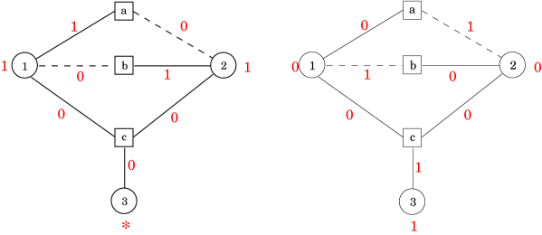
Figure 7: A simple SAT problem with three variables, two 2-clauses, one 3-clause, and loops. Each figure gives one of the two possible solutions of warning propagation. The number on each edge $(a,i)$ is the warning $u_{a\to i}$, the number next to each variable node is the corresponding generalized state of the variable in each of the two ’clusters’. The SP equations for this graph have an infinite number of solutions, with $\eta_{a\to 1}=\eta_{b\to 2}=x$, $\eta_{a\to 2}=\eta_{b\to 1}=y$, $\eta_{c\to 1}=\eta_{c\to 2}=0$, and $\eta_{c\to 3}=(1-x)^{2}y^{2}/(1-xy)^{2}$

Two conjectures arise naturally from the heuristic statistical physics approach and the numerical experiments on SP. They should hold for the random satisfiability problem, in the large $N$ limit, in some hard SAT window of $\alpha$ just below $\alpha_{c}$ :

• 1) With probability one (on the set of initial messages), SP converges to a unique set of fixed point messages.

• 2) These fixed point messages contain the correct information about the constrained clusters, and in particular the number of constrained clusters can be computed as in (39).

Note that for finite $N$, there are obvious counterexamples to these conjectures, as shown in fig. 7.

VI Comments and perspectives

When the solutions of a SAT (or more generally of a constrained satisfaction problem) tend to cluster into well separated regions of the assignment space, it often becomes difficult to find a global solution because (at least in all local methods), different parts of the problem tend to adopt locally optimal configurations corresponding to different clusters, and these cannot be merged to find a global solution. In SP we proceed in two steps. First we define some elementary messages which are warnings, characteristic of each cluster, then we use as the main message the surveys of these warnings. The warning that we used is a rather simplified object: it states which variables are constrained and which are not constrained. Because of this simplification the surveys can be handled easily, which makes the algorithm rather fast. As we saw in sect.V, one might also aim at a finer description of each cluster, where the elementary messages would give the probability that a variable is in a given state ($\in\{0,1\}$), when considering the set of all SAT configurations inside this given cluster. In this case the survey will give the probability distribution of this probability distribution, when one chooses a cluster randomly. This is more cumbersome algorithmically, but there is no difficulty of principle in developing this extension. One could also think of generalizing further the messages (to probability distributions of probability distributions of probability distributions), if some problems have a structure of clusters within other clusters (this is known to happen for instance in spin glasses MPV ), but the cost in terms of computer resources necessary to implement it might become prohibitive.

We have presented here a description of a new algorithmic strategy to handle the SAT problem. This is a rather general strategy which can also be applied in principle, to all Constraint Satisfaction Problems coloring ; MZ_pre . At the moment the approach is very heuristic, although it is based on a rather detailed conjecture concerning the phase structure of random 3-SAT. The validity of a similar conjecture has been checked exactly in the random XOR-SAT problem. It would be interesting to study this algorithmic strategy in its own, independently from the random 3-SAT problem and the statistical physics study. One can expect progress on SP to be made in the future in various directions, among which: Rigorous results on convergence, different ways of using the information contained in the surveys, generalization of the algorithm to deal with complex graphs which are not typical random graphs, use of the generalized SP with penalty to provide UNSAT certificates. The generalization of SP to generic Constraint Satisfaction Problems is discussed in a separate publication BMWZ .

References

- (1) S.A. Cook, D.G. Mitchell, Finding Hard Instances of the Satisfiability Problem: A Survey, In: Satisfiability Problem: Theory and Applications. Du, Gu and Pardalos (Eds). DIMACS Series in Discrete Mathematics and Theoretical Computer Science, Volume 35, (1997)
- (2) E. Friedgut, J. Amer. Math.Soc. 12, 1017 (1999)
- (3) O. Dubois, Y. Boufkhad, J. Mandler, Typical random 3-SAT formulae and the satisfiability threshold, Proceedings of the eleventh annual ACM-SIAM symposium on Discrete algorithms, p.126-127, January 09-11, 2000, San Francisco, California (US)
- (4) A.C. Kaporis, L. M. Kirousis, E.G. Lalas, The probabilistic analysis of a greedy satisfiability algorithm, Proceedings of the 10th Annual European Symposium on Algorithms, Lect. Notes in Computer Science,Sringer-Verlag (London, UK), 574-585 (2002)
- (5) C. Moore, D. Achlioptas, Random k-SAT: Two Moments Suffice to Cross a Sharp Threshold, preprint, extended abstract in FOCS’02, 779-788 (2002)
- (6) D. Achlioptas, Y. Perez, The Threshold for Random k-SAT is to appear in JAMS, Extended Abstract in STOC’03, 223-231 (2003)
- (7) R. Monasson, R. Zecchina, Phys. Rev. E 56, 1357 (1997); R. Monasson, R. Zecchina, Phys. Rev. Lett. 76, 3881 (1996)
- (8) G. Biroli, R. Monasson, M. Weigt, Europ. Phys. J. B 14, 6118 (2000)
- (9) O. Dubois, R. Monasson, B. Selman R. Zecchina (Eds.), Phase Transitions in Combinatorial Problems, Theoret. Comp. Sci. 265 (2001).
- (10) S. Kirkpatrick, B. Selman, Critical Behaviour in the satisfiability of random Boolean expressions, Science 264, 1297 (1994)
- (11) J.A. Crawford L.D. Auton, Experimental results on the cross-over point in random 3-SAT, Artif. Intell. 81, 31-57 (1996).
- (12) R. Monasson, R. Zecchina, S. Kirkpatrick, B. Selman and L. Troyansky, Nature (London) 400, 133 (1999).
- (13) M. Mézard, G. Parisi and R. Zecchina, Science 297, 812 (2002) (Sciencexpress published on-line 27-June-2002; 10.1126/science.1073287)
- (14) M. Mézard and R. Zecchina, Random 3-SAT: from an analytic solution to a new efficient algorithm, Phys. Rev. E 66 (2002) 056126.
- (15) J. Pearl, Probabilistic Reasoning in Intelligent Systems, 2nd ed. (San Francisco, MorganKaufmann,1988)
- (16) M. Mézard, G. Parisi,The Bethe lattice spin glass revisited Eur.Phys. J. B 20, 217–233 (2001), M. Mézard, G. Parisi,The cavity method at zero temperature, J. Stat. Phys. 111, 1 (2003)
- (17) H.O. Georgii, Gibbs Measures and Phase Transitions, De Gruyter Studies in Mathematics Vol. 9. Berlin: de Gruyter 1988. Russian edition: Mir 1992
- (18) M. Talagrand, Rigorous low temperature results for the p-spin mean field spin glass model, Prob. Theory and Related Fields 117, 303–360 (2000).
- (19) S. Franz and M. Leone, Replica bounds for optimization problems and diluted spin systems, J. Stat. Phys. 111, 535 (2003)
- (20) M. Mézard, F. Ricci-Tersenghi, R. Zecchina, Alternative solutions to diluted p-spin models and XOR-SAT problems, J.Stat. Phys. 111, 505-533 (2003)
- (21) S. Cocco, O. Dubois, J. Mandler, R. Monasson, Rigorous decimation-based construction of ground pure states for spin glass models on random lattices, Phys. Rev. Lett. 90, 047205 (2003)
- (22) A. Braunstein, M. Leone, F. Ricci-Tersenghi, R. Zecchina. Complexity transitions in global algorithms for sparse linear systems over finite fields, J. Phys. A 35, 7559 (2002)
- (23) F.R. Kschischang, B.J. Frey, H.-A. Loeliger, Factor Graphs and the Sum-Product Algorithm, IEEE Trans. Infor. Theory 47, 498 (2002).
- (24) R. Mulet, A. Pagnani, M. Weigt, R. Zecchina, Coloring Random Graphs, Phys. Rev. Lett. 89, 268701 (2002)
- (25) R. G. Gallager, Low-Density Parity-Check Codes Cambridge, MA: MIT Pres,1963.
- (26) B. Selman, H. Kautz, B. Cohen, Local search strategies for satisfiability testing, in: Proceedings of DIMACS, p. 661 (1993).
- (27) Satisfiability Library: www.satlib.org/
- (28) D. E. Knuth, The art of computer programming, vol. I: fundamental algorithms, (Addison-Wesley, New-York, 1968)
- (29) www.ictp.trieste.it/zecchina/SP
- (30) J.S. Yedidia, W.T. Freeman and Y. Weiss, Generalized Belief Propagation, in: Advances in Neural Information Processing Systems 13, T.K. Leen, T.G. Dietterich, and V. Tresp (Eds.), MIT Press 2001, pp. 689-695.
- (31) Mézard, M., Parisi, G., Virasoro, M.A., Spin Glass Theory and Beyond, World Scientific, Singapore (1987).
- (32) A. Montanari, G. Parisi, F. Ricci-Tersenghi, J. Phys. A 37, 2073 (2004)
- (33) S. Mertens, M. Mezard, R. Zecchina, Threshold values for random K-SAT from the cavity method, preprint http://arXiv.org/cs.CC/0309020 (2003)
- (34) G. Parisi, A backtrack survey propagation algorithm for K-satisfiability‘, preprint http://arXiv.org/cond-mat/0308510 (2003)
- (35) A. Braunstein, R. Zecchina, J. Stat. Mech: Theory and Experiment (JSTAT), p06007 (2004)
- (36) A. Braunstein, M. Mezard, M. Weigt, R. Zecchina, Survey propagation for general Constraint Satisfaction Problems, Volume on Computational Complexity and Statistical Physics, Oxford University Press,Santa Fe Institute Studies in the Sciences of Complexity (2003), ArXiv: lanl/arXiv.org/cond-mat/0212451
- (37) G. Parisi, On the survey-propagation equations for the random K-satisfiability problem, preprint, attp://arXiv.org/cs.CC/0212009 (2002)