Algorithmic scalability in globally constrained conservative parallel discrete event simulations of asynchronous systems

Abstract

We consider parallel simulations for asynchronous systems employing $L$ processing elements that are arranged on a ring. Processors communicate only among the nearest neighbors and advance their local simulated time only if it is guaranteed that this does not violate causality. In simulations with no constraints, in the infinite $L$-limit the utilization scales (Korniss et al, PRL 84, 2000); but, the width of the virtual time horizon diverges (i.e., the measurement phase of the algorithm does not scale). In this work, we introduce a moving $\Delta$-window global constraint, which modifies the algorithm so that the measurement phase scales as well. We present results of systematic studies in which the system size (i.e., $L$ and the volume load per processor) as well as the constraint are varied. The $\Delta$-constraint eliminates the extreme fluctuations in the virtual time horizon, provides a bound on its width, and controls the average progress rate. The width of the $\Delta$-window can serve as a tuning parameter that, for a given volume load per processor, could be adjusted to optimize the utilization so as to maximize the efficiency. This result may find numerous applications in modeling the evolution of general spatially extended short-range interacting systems with asynchronous dynamics, including dynamic Monte Carlo studies.

I INTRODUCTION

Parallel Discrete Event Simulations (PDES) of asynchronous systems is a computer science term that stands for parallel simulations of complex systems with asynchronous dynamics. Such spatially extended complex interacting systems appear across a wide range of fields in natural sciences, and their examples include interacting spin systems in material physics, activated processes in chemistry, contact processes in stochastic epidemic models, stochastic market models in finance, scheduling call arrivals in communication networks, and routing problems in internet traffic, to mention just a few applications of PDES. Despite active research in this area Fuji90 ; NF94 very few of the PDES techniques have filtered through to the physics community. Even the simplest random-site update Monte Carlo schemes BH97 , where updates correspond to Poisson-random discrete events, were long believed to be inherently serial (at least in the physics community). Simulation studies of parallel computations for asynchronous distributed systems date back more than two decades ago CM79 ; CM81 . However, it was Lubachevsky’s work Lub87 ; Lub88 on parallel simulations of dynamic Ising spin systems which shed a new light on this old problem and showed how to efficiently perform conservative simulations on a parallel computer. The design of efficient algorithms that would allow modeling of asynchronous systems in a parallel processing environment is even more important nowadays, when parallel architectures have become generally available. The architectures of today may consist of several thousands of processing elements, but the size of future systems may be of the order of hundred thousands blue02 . Such architectures pose new questions of algorithm efficiency and scalability in large scale massively parallel processing. We address these questions for conservative PDES, using the tools of modern statistical physics, in particular, those of non-equilibrium surface growth BS95 .

The difficulties of parallelizing spatially extended asynchronous cellular automata arise because in asynchronous systems the discrete events are not synchronized by a global clock. For example, in the basic dynamic Ising model for ferromagnets discrete spins with two states each are placed on a lattice. The discrete events are attempted spin flips, where the spin-flip probability at some site depends on the energy states of the neighboring sites. The lattice can be partitioned into a number of sub-lattices, and each sub-lattice may be assigned to a different processor. Processing elements (PE) attempt a number of randomly chosen spin-flips, and communicate with each other in some update attempts (a discrete event). Each PE carries its own local virtual time which is advanced by every update attempt. The local virtual time on a PE is the simulated time at the spins on its sub-lattice. In the conservative PDES implementation it is ensured that causality is not violated before each PE makes an update attempt. Alternatively, in an optimistic PDES implementation, PEs make updates without communicating with the neighbors, thus sometimes causing causality errors. The optimistic scheme provides a recovery mechanism by undoing the effects of all events that have been precessed prematurely. Optimistic PDES have been an object of theoretical and simulation studies FK91 ; Nico91 ; Stei93 ; Stei94 ; Stei96 . The development of spatio-temporal correlations and self-organized criticality have been recently studied in the optimistic simulations of the dynamics of Ising spin systems SOS01 ; OSS01 . The conservative scheme has been used recently to model magnetization switching KNR99 , ballistic particle deposition LP96 , and a dynamic phase transition in highly anisotropic thin-film ferromagnets KWRM01 ; KRN02 . These recent applications suggest that the conservative scheme should be particularly efficient when applied to large systems with short-range interactions.

Early efficiency studies of the conservative scheme Lub89 ; Nico93 do not identify the mechanism which would ensure the scalability of the PDES for an arbitrary system size. Recently, Korniss et al KTNR00 introduced a new approach that exploits an analogy between the virtual time horizon and a fluctuating surface that grows in a deposition process. In this picture, the fraction of non-idling PEs (the utilization) exactly corresponds to the density of local minima in a virtual time surface. They showed that, in the case of one spin site per PE, the steady state virtual time surface is governed by the Edwards-Wilkinson Hamiltonian, implying that the utilization does not vanish for an infinitely large system of PEs. Ignoring communication delays and assuming that the utilization is equivalent to the efficiency, they concluded that the computation phase of short-ranged conservative PDES is asymptotically scalable. In general, the utilization should not be taken as a sole measure of efficiency in the modeling of asynchronous systems. The same analysis of a virtual time surface KTNR00 ; KNKG02 ; KNTR01 ; KNRGT02 demonstrated that, in the case of one site per PE, the virtual time horizon infinitely roughens in the infinite PE-limit. The statistical spread of the virtual time surface severely limits an averaging or measurement phase of PDES, and divergence leads to severe difficulties with data management. Therefore, while the simulation phase (as determined by the utilization studies) is asymptotically scalable, the measurement phase is not. To ensure the efficiency of the algorithm, solutions need to be sought in which both phases of the computation are scalable.

In studies of asynchronous updates in large parallel systems, Greenberg et al GSS96 proposed a $K$-random connection model, where at each time step each PE randomly connects with $K$ other PEs in the system. The virtual time horizon for this model is short-range correlated and has a finite width in the infinite PE-limit. Encouraged by this result, we considered the two alternative modifications to the conservative scheme: a random connection model KNGTR and the moving window constraint KNKG02 . The purpose of these modifications is to ensure that the measurement phase of the conservative PDES is scalable.

This paper presents the results of systematic simulation studies of conservative asynchronous PDES with the moving window constraint (i.e., simulation studies of the simulations). In Section II we define terminology and we outline both the basic conservative update scheme and the constraint update rule that we use in modeling of asynchronous PDES. The scheme that we consider is such that the evolution of the time horizon is decoupled from the underlying systems. The only one assumption that we make about underlying complex systems is that they are characterized by short-range interactions. Therefore, our analysis is generally valid for a wide spectrum of physics applications. Section III contains the analysis of scalability issues, which is based on analogies between PDES and kinetic roughening in non-equilibrium surface growth. In the PDES analysis the focus is placed on two major issues: the scaling of the simulation phase and the scaling of the measurement phase. In Section IV we present and analyze numerical data that were obtained in large scale simulations of an asynchronous conservative PDES scheme with a moving window constraint. In our time evolution studies, we simultaneously varied the width of the moving window and the system size (i.e., the number of processing elements in the system as well as the number of volume elements per processing element) in search for regularities that would allow general conclusions. In Section V, we discuss connections between the scalability of a constrained conservative scheme and the design of highly efficient algorithms for asynchronous systems.

II CONSERVATIVE PDES FOR SPATIALLY DECOMPOSABLE CELLULAR AUTOMATA

We consider an ideal system consisting of $L$ identical PEs, arranged on a ring. Each PE has $N_{V}$ lattice sites (or operation volumes) and the algorithm randomly picks one of the $N_{V}$ sites. If the site that is picked is an end site communication with a neighboring PE is required, while no communication between PEs is required if an interior site is picked. For this system a discrete event means an update attempt that takes place instantaneously. The state of the system does not change between update attempts. Processing elements perform operations concurrently, however, update attempts are not synchronized by a global clock. Such a system can represent, for example, concurrent operations of random spin flipping in a large spatially extended ensemble that can be arranged on a regular lattice. In this picture, the ensemble is spatially decomposed into $L$ subsystems, each of which carries $N_{V}$ sites. Each subsystem is carried by one PE and the required communication is the exchange of information about states of the border spins. In the simplest case there is one site per PE, $N_{V}=1$, the system is a closed spin chain, and a spin-flip attempt at the $k$-th PE depends on the two nearest-neighbor spins located on the $(k-1)$-th and the $(k+1)$-th PEs. The $k$-th PE may not perform an update until it receives information from these neighboring PEs.

In this conservative PDES scheme, to simulate asynchronous dynamics employing $L$ processors, each $k$-th PE generates its own local simulated time $\tau_{k}$ for the next update attempt. Update attempts are simulated as independent Poisson-random processes, in which the $k$-th local time increment (i.e., the random time interval between two successive attempts ) is exponentially distributed with unit mean. A processor is allowed to update its local time if it is guaranteed not to violate causality. Otherwise, it remains idle. The time step $t$ is the index of the simultaneously performed update attempt. It corresponds to an integer wall-clock time with each processor attempting an update at each value of $t$.

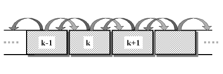
Figure 1: Short range connections in PDES for a linear chain.

The simplest choice for a communication rule between processors, which is faithful to the original dynamics of the underlying system, is a short-range connection model (Fig. 1), where, at any time step $(t+1)$, the $k$-th PE is allowed to update if its local simulated time ${\tau_{k}}(t)$ is not greater than the local simulated times of its two nearest neighbors:

$$\tau_{k}(t)\leq\min\left\{\tau_{k-1}(t),\tau_{k+1}(t)\right\}.$$ (1)

The periodicity condition requires communication between the first and the last PEs. In effect, this update rule introduces a nearest neighbor interaction and corresponding correlations between PEs, which is analogous with non-equilibrium surface growth. It was shown KTNR00 that in the case of $N_{V}=1$ the evolution of the virtual time horizon on coarse-grain length scales is governed by the Kardar-Parisi-Zhang (KPZ) equation KPZ86 :

$$\partial_{t}\tau=\partial_{xx}\tau-\lambda\left(\partial_{x}\tau\right)^{2}+\eta(x,t),$$ (2)

where $x$ is a spatial variable in a continuum limit, the constant $\lambda$ is related to the coarse-graining procedure, and $\eta(x,t)$ accounts for random fluctuations.

In PDES with a moving window constraint, the communication pattern between processing elements remains the short-range connection type but the new update rule requires that additionally at each $(t+1)$-step the local simulated time of the $k$-th processor fits within a window of width $\Delta$ that is defined relative to the slowest PE (i.e., the one with the smallest $\tau$) at time $t$. Explicitly, the $k$-th PE is allowed the update if $\tau_{k}(t)$ simultaneously satisfies the short-range connection condition (1) and the following window condition:

$$\tau_{k}(t)\leq\Delta+\min\left\{\tau_{k}(t):k=1,\dots,L\right\}.$$ (3)

In the computer science community the minimum in Eq.(3) is called the global virtual time FK91 ; Nico91 ; Stei93 ; Stei94 . From this definition it follows that the short-range connection model can be viewed as a particular case of the original update scheme when the width of the window is set to infinity, in which case condition (3) is trivially satisfied for all times. Thus an infinite window is equivalent to the absence of the constraint.

In typical simulations, when the number of volume elements $N_{V}$ is larger than the minimum $N_{V}=1$, a causality condition (1) is enforced only for the border volumes on each PE. If, at any $t$-step, a randomly chosen volume element happens to be from the interior, i.e., when all of its immediate neighbors reside on one PE, then the PE always executes the update and its local time is incremented for the consecutive update attempt: $\tau_{k}(t+1)=\tau_{k}(t)+\eta_{k}(t)$, where $\eta_{k}$ is the $k$-th random time increment that is exponentially distributed, randomly chosen independently on each PE and at each parallel step $t$. In the constrained simulations, condition (3) is enforced for any randomly chosen volume element.

In the conservative update scheme a causality requirement is the main mechanism that generates correlations among processing elements. In the absence of a causality requirement local simulated times would be incremented independently of each other in the fashion of random deposition (RD) BS95 . However, even with this RD update rule, imposing the windowing condition (3) alone will give rise to correlations among processors. Note that the RD update rule does not belong to a class of conservative update schemes i.e., it cannot faithfully simulate the underlying system dynamics. For $\Delta$-constrained RD simulations, the speed with which the correlations spread among all PEs is determined by the width of the $\Delta$-window.

For a set of $L$ processing elements, a simulated time horizon (STH) is defined as a set of $L$ local simulated times at a time step $t$. To study the roughening of the STH surface, we monitor the surface width $\langle w(t)\rangle$, which is defined in standard fashion BS95 via the variance of the STH:

$$\langle w^{2}(t)\rangle=\left\langle\frac{1}{L}\sum_{k=1}^{L}\left(\tau_{k}(t)-\bar{\tau}(t)\right)^{2}\right\rangle,$$ (4)

where the angle bracket denotes an ensemble average and $\bar{\tau}$ denotes the mean virtual time, $\bar{\tau}(t)=\frac{1}{L}\sum_{k=1}^{L}\tau_{k}(t)$. Alternatively, the surface width can also be defined as the absolute standard deviation $\langle w_{a}(t)\rangle$ from the mean virtual local time:

$$\langle w_{a}(t)\rangle=\left\langle\frac{1}{L}\sum_{k=1}^{L}\left|\tau_{k}(t)-\bar{\tau}(t)\right|\right\rangle.$$ (5)

We use both definitions (4-5) in our analysis. To study the efficiency of an update process in the system of $L$ processors, we define the utilization $\langle u_{L}(t)\rangle$ as a fraction of processors that performed an update at parallel time-step $t$. Throughout the paper we consistently use the following notation: the surface width $\langle w(t)\rangle$ is an ensemble average of $w(t)=\sqrt{w^{2}(t)}$ computed at $t$, while $\langle w\rangle$ denotes the corresponding steady-state value at $t\to\infty$. The subscript “a” denotes the width computed in accordance to (5), while subscripts “$L$” or “$N_{V}$” (e.g., $\langle w_{L,N_{V}}\rangle$) indicate the parameter dependance of the width computed in accordance to (4).

III SCALABILITY MODELING

There are two important aspects of scalability, which should be dealt with in studies of algorithm efficiency. Both of them regard the time in the system and connect with data management issues. The first is the question of whether or not the utilization reaches a constant non-zero value in the limit of large system size (when $L$ and $N_{V}$ may arbitrarily vary). In particular, one needs to know if the “worst case scenario” of one volume element per PE can produce a non-zero utilization in the infinite $L$-limit. A zero value of utilization in the infinite system size limit would suggest that an algorithm would likely be useless for computationally intensive tasks on future generations of massively parallel computers, i.e., on systems that contain hundreds of thousands of processing elements blue02 . The second question is the behavior of the evolution of the STH, whether or not the statistical spread of the STH saturates in time or scales with the system size. A negative answer to the latter question would suggest that an algorithm would probably prove impractical in actual applications, because the divergence of the STH width implies that, for most computationally intensive jobs, the data collection and averaging would impose a memory requirement per PE in excess of hardware capacities.

In our scalability studies we exploit existing analogies between the time evolution of the STH and kinetic roughening in non-equilibrium surface growth; and we use selected results of non-equilibrium surface studies BS95 ; HZ95 ; Krug97 in analyzing the stochastic behavior of the system under consideration. The conservative short-range communication scheme between the system components can be regarded as an effective short-range interaction among PEs and treated in a similar manner to an interaction among sites of any non-equilibrium surface, growing on a regular lattice. For these surfaces, the lateral correlation length $\xi$ between sites follows the power law $\xi\sim t^{1/z}$, where $z$ is the dynamic exponent. For a finite system, $\xi$ cannot grow beyond the system size $L$ and it is observed that for times much smaller than a cross-over time $t_{\times}$, $t_{\times}\sim L^{z}$, the surface width increases in accordance to $t^{\beta}$, where $\beta$ is the growth exponent. For times much larger than the cross-over time, the surface width saturates and scales as $L^{\alpha}$, where $\alpha$ is the roughness exponent. The exponents satisfy the scaling relation: $z\beta=\alpha$. The values of the exponents are independent of the details of the system and of the nature of the interactions between sites. Their values can be determined from the corresponding stochastic growth equation, which defines the universality class. We observed that the simulated time horizon shows kinetic roughening and the typical scaling behavior KNKG02 :

$$\langle w_{L}^{2}(t)\rangle \sim t^{2\beta}\quad\text{for $t\ll t_{\times}$,}$$ (6)

$$\langle w_{L}^{2}(t)\rangle \sim L^{2\alpha}\quad\text{for $t\gg t_{\times}$.}$$ (7)

It was demonstrated in KTNR00 that in the case of one site per PE (i.e., $N_{V}=1$) the time evolution of the STH in the short-range connection model (1) follows the KPZ equation (2) and direct simulations confirmed that the scaling exponents in Eqs. (6-7) have values consistent with the KPZ universality class ($\alpha=1/2$ and $\beta=1/3$).

III.1 Steady-state scaling for utilization

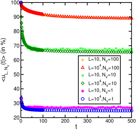
Figure 2: Unconstrained PDES: Time evolution of the mean utilization $\langle u(t)\rangle$ (averaged over $N=1024$ independent random trials) for various system sizes: $L=10$ and $10^{4}$ and $N_{V}=1,10$ and $100$.

As the time index advances the utilization falls from its initial maximal value at $t=0$. Figure 2 presents the time evolution of the utilization for various system sizes in the basic PDES with short-range connections with the infinite $\Delta$-window. For each of the system size, the utilization attains a steady-state, characterized by a non-zero value in the infinite $t$-limit. This qualitative result is also true for the simulations in two and three dimensions, when an individual PE is allowed to connect with four and six immediate neighbors, respectively KNTR01 . Such a non-zero steady-state value is characteristic for the KPZ universality class and can be expressed by the Krug and Meakin KM90 relation for generic KPZ-like processes:

$$\lim_{t\to\infty}\langle u_{L}(t)\rangle\approx\langle u_{\infty}\rangle+\frac{const.}{L^{2(1-\alpha)}},$$ (8)

where $\langle u_{\infty}\rangle$ denotes the utilization in the infinite $L$-limit. Toroczkai et al TKDZ00 showed that the basic conservative PDES with one site per PE satisfies relation (8), and they used it to extrapolate their utilization data to large $L$. Their value for the utilization in the infinite PE-limit is $\langle u_{\infty}\rangle=24.6461(7)\%$ KTNR00 ; KNKG02 . This finding demonstrates that the simulation part of the algorithm is scalable in the case of the 1-d conservative PDES with the minimal number of volume elements per PE. Explicitly, this means that even in the worst case scenario, it is possible to run simulations arbitrarily long with a non-zero average rate of progress. In the case of 2-d and 3-d PDES, the roughness exponents are $\alpha=0.2-0.4$ (in 2-d) and $\alpha=0.08-0.3$ (in 3-d) KNTR01 , and the $N_{V}=1$ steady-state utilization can be estimated as $\langle u_{\infty}\rangle\cong 12\%$ and $\langle u_{\infty}\rangle\cong 7.5\%$, respectively KNTR01 .

III.2 The evolution of the simulated time horizon

The unconstrained PDES are characterized by an infinite roughening of the STH surface in the limit of infinite system size. Figure 3 presents a typical time evolution of a surface generated by this basic update scheme for $N_{V}=1$ and $L=100$. As the time index advances, the surface grows and the statistical spread of its interface increases in accordance with Eqs. (6-7). Figure 4 shows the time evolution of the surface width for a few selected system sizes. For a fixed system size the width follows relations (6-7): after the initial growth phase, the surface saturates and its width reaches the plateau value. By comparing the widths for $N_{V}=1$ (Fig. 4a) to those for $N_{V}=10$ (Fig. 4b), one can see that for a fixed $L$-number of PEs, increasing the number of sites per PE shifts the cross-over time $t_{\times}$ to later values and increases the value of the width at the plateau. This is expected since a larger value of $N_{V}$ yields a larger cumulative value for the local time increment between two successive communications with neighboring PEs. In the case of $N_{V}=1$, the width of the STH approaches a finite constant for a finite $L$-number of PEs; however this constant diverges in the infinite $L$-limit in the power law fashion:

$$\langle w^{2}\rangle\sim L^{2\alpha},$$ (9)

which gives the linear divergence of the surface variance for the KPZ universality class. The same holds for the extreme fluctuations above and below the mean simulated time KTNR00 . This finding is also valid in the case when each PE carries a block of sites. The above scaling behavior creates difficulties when intermittent data on each PE have to be stored until all PEs reach the simulated time instant at which statistics collection is performed (e.g., a simple averaging over the full physical application). The diverging spread of the time horizon implies a diverging storage need for this purpose on every PE. Thus, the diverging width of the STH means that the memory requirement per processing element, for temporary data storage, diverges as the number of processing elements gets arbitrarily large. Therefore, the measurement phase of an algorithm that follows the basic conservative update scheme is asymptotically not scalable. In actual applications, the programmer must seek some means of constraining the infinite roughening of the STH or must impose some global synchronization on the system of PEs.

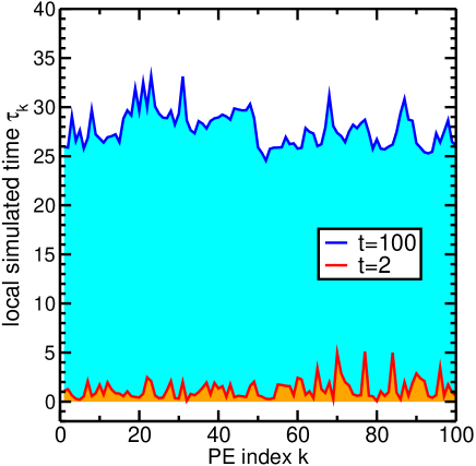
Figure 3: Unconstrained PDES: Time evolution of the time horizon for $L=100$ PEs and $N_{V}=1$ sites per PE. The lower surface is a snapshot at $t=2$, the upper surface is a snapshot at $t=100$. For $L=100$ the crossover time is $t_{\times}\approx 3700$.

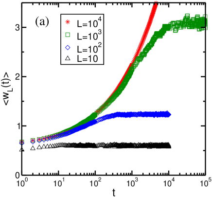
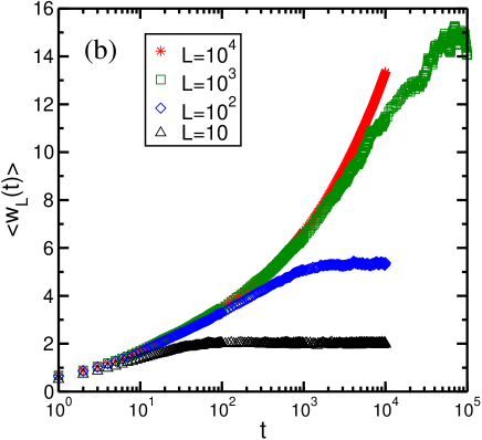
Figure 4: Unconstrained PDES: Time evolution of the mean surface width $\langle w(t)\rangle$ of the STH (averaged over $N=1024$ independent random trials) for various number $L$ of PEs, in simulations with: (a) $N_{V}=1$ site per PE; (b) $N_{V}=10$ sites per PE. Since the plateau has been reached for $L=10$ and $L=100$, the times $t$ larger than $10^{4}$ are not shown. For $L=10^{4}$, the plateau is reached for $t$ larger than $10^{6}$.

Our and Lubachevsky’s earlier studies show that to make the conservative scheme efficient, one must use a large number of volume elements $N_{V}$. It is expected that an increase in $N_{V}$ will modify the growth phase of the STH. In the case of large $N_{V}$, the initial growth phase (for $0<t<t_{1}$) should be characterized by $\beta=1/2$, typical for the RD universality class. Then, after the first cross-over time $t_{1}$ (for $t_{1}<t<t_{2}$, where $t_{2}$ is the saturation time) the growth should be characterized by $\beta=1/3$, typical for the KPZ universality class. In this way, making the simulation phase more efficient (by increasing $N_{V}$) will speed up the initial growth. Thus, the state savings, which are traditionally associated with optimistic schemes, are disadvantageous in conservative schemes.

IV CONSERVATIVE PDES WITH THE MOVING WINDOW CONSTRAINT

A standard way of controlling the growth of the STH is to impose a constraint on its width in the spirit of parallel simulations of asynchronous cellular automata that was proposed by Lubachevsky Lub87 ; Lub88 . A straightforward application of this idea is the $\Delta$-constrained update scheme which demands that at each update attempt a PE can perform an update only if its value of $\tau_{k}$ is within the window. The effect of condition (3) is that fast PEs are forced to postpone their updates until slower PEs catch up. In the simplified version studied here, the assigned distance apart is measured in terms of the processor local time that is compared to the global minimum virtual time. Since at each $t$ the global minimum of the STH changes its location, so does the window for the update. In this sense a moving window constraint can be considered as an implicit rule that induces global synchronization, in which each PE connects with the slowest PE. From the implementation point of view, the most important questions are the scalability issues for realistic systems, where each PE may carry an arbitrary number of sites, because mainly these issues will determine the efficiency of the algorithm in actual applications.

IV.1 Simulation phase

In the $\Delta$-constrained PDES, simulations reach a steady state for an arbitrary system size in a similar fashion as in the basic short-range connection model, illustrated in Fig. 2. In general, for any $\Delta$-value, when $L$ is fixed the steady state value of the utilization gets larger as $N_{V}$ gets larger; and, when $N_{V}$ is fixed it gets smaller as $L$ is increased. This behavior reflects the strength of the correlations between PEs which arise due to the update rule (1). Namely, for fixed $L$, the frequency of an update per PE increases as $N_{V}$ increases because condition (1) does not need to be verified for the internal sites and the probability of randomly choosing a border site is $1/N_{V}$. Therefore, in this case, correlations that arise due to the short-range connections between PEs weaken when $N_{V}$ is increasing. In the infinite $N_{V}$-limit these correlations become negligible and the process of incrementing local simulated times resembles random deposition on the 1-d lattice of size $L$. Thus, the RD-limit is equivalent to the infinite $N_{V}$-limit of PDES.

The mean steady state utilization $\langle u_{L,N_{V}}\rangle$ as a function of the system size is presented in Fig. 5. When the number $N_{V}$ of sites per PE is increased the curves converge towards the RD limit. With a narrow $\Delta$-window (Fig. 5a) the RD limit is approached fairly quickly (with $N_{V}=100$ for $\Delta=10$), while with a wide $\Delta$-window (Fig. 5b) the RD limit is approached more slowly. For an infinite $\Delta$-window the RD limit is $\langle u_{L,\infty}\rangle=100\%$, which is the effect of no-correlations in the system in this limiting case. Obviously, $\langle u_{L}\rangle=1/L\times 100\%$ when $\Delta=0$, because in this case only one PE is allowed to make an update. The RD curves in Fig. 5 display the steady state utilization for simulations that are governed only by the update rule (3) alone, i.e., in the absence of other communications between processing elements. The fall off in the RD utilization values with an increase in the number of PEs, indicates the strength of correlations between PEs, which exclusively results from imposing the $\Delta$-window constraint. When all three parameters, $\Delta$, $L$ and $N_{V}$, are allowed to vary in conservative PDES, the value of the utilization is mostly determined by the width of the moving window. The choice of a very narrow $\Delta$-window severely suppresses the average progress rate.

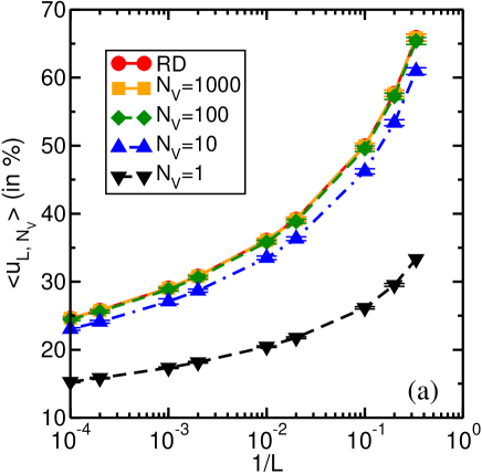
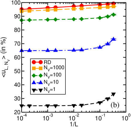
Figure 5: Mean steady state utilization $\langle u\rangle$ in constrained PDES as a function of the system size for the $\Delta$-window size: (a) $\Delta=10$; (b) $\Delta=100$. $L$ is the number of PEs. When the number $N_{V}$ of sites per PE is increased the curves converge towards the RD limit.

To determine a scaling relation for the steady state utilization in the infinite PE-limit, we analyzed the mean steady state utilization $\langle u_{L}\rangle$ as a function of $1/L$ for several values of $\Delta$ and $N_{V}$, in each case performing a standard rational function interpolation PTVF92 of the simulation data:

$$\langle u_{L}\rangle = \frac{a_{0}+\sum_{k=1}^{K_{n}}a_{k}\left(\frac{1}{L}\right)^{k}}{1+\sum_{k=1}^{K_{d}}b_{k}\left(\frac{1}{L}\right)^{k}}$$

$$= \frac{a_{0}}{1+\sum_{k=1}^{K_{d}}b_{k}\left(\frac{1}{L}\right)^{k}}+\frac{a_{1}}{L}\frac{1+\sum_{k=1}^{K_{n}-1}\frac{a_{k+1}}{a_{1}}\left(\frac{1}{L}\right)^{k}}{1+\sum_{k=1}^{K_{d}}b_{k}\left(\frac{1}{L}\right)^{k}},$$

where the polynomial degrees $K_{n}$ and $K_{d}$ were varied to determine the best set of the interpolation coefficients. Then, knowing the leading coefficients $a_{0}$ and $a_{1}$, we extrapolated the utilization values to $L=\infty$. In the infinite $L$-limit the leading term in Eq. (IV.1) is $\langle u_{\infty}\rangle\equiv a_{0}$ and we obtain the following scaling relation:

$$\lim_{L\to\infty}\langle u_{L}\rangle=\langle u_{\infty}\rangle+\frac{const.}{L}.$$ (11)

The mean utilization $\langle u_{\infty}\rangle$ in the infinite $L$-limit, as a function of $N_{V}$ and the $\Delta$-window size, is presented in Fig. 6. Data points for $N_{V}=10^{8}$ represent extrapolated values for the $\Delta$-constrained RD simulations. It can be observed that in the infinite $L$-limit, as well as at each update attempt and in the saturation limit, the utilization is strongly affected by the value of $\Delta$. A narrow $\Delta$-window can significantly slow down the system because a significant number of PEs (that otherwise would perform an update) may be constrained to wait for the slowest ones to catch up. This effect is particularly noticeable when the number $N_{V}$ of sites per PE becomes large. For example, for $N_{V}=100$, when the $\Delta$-window is narrowed to $\Delta=1$, the utilization may drop by as much as $65\%$ from its value at $\Delta=100$. When $\Delta=0$, $\langle u_{\infty}\rangle=0$ for any $N_{V}\geq 1$.

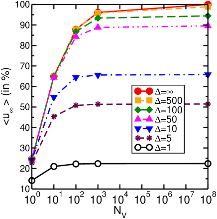
Figure 6: Mean utilization $\langle u_{\infty}\rangle$ in the limit of $L\to\infty$ as a function of the number of volume elements $N_{V}$ and the $\Delta$-window size. Data points for $N_{V}=10^{8}$ present the constrained RD simulations. Symbols represent the simulation data. The lines are guides for the eyes.

The standard $\%$-error in our simulation data for the utilization at each $t$-step does not exceed $1\%$ when configurational averages are extracted from $N=1024$ independent random trials, except for the data obtained with the infinite window, which are within a $2\%$ error bar (due to a smaller $N$). We estimate that our values for the steady state utilization in the infinite $L$-limit are well within a $2\%$ relative uncertainty. The utilization data that are presented in Fig. 6 can be fitted to the approximate formula:

$$u(N_{V},\Delta)=u_{RD}(\Delta)\times u_{KPZ}({N_{V}})^{p(\Delta,N_{V})},$$ (12)

where the first factor approximates the utilization curve in the RD limit, $u_{RD}(\Delta)=\lim_{N_{V}\to\infty}u(N_{V},\Delta)$. The base in the second factor approximates the utilization curve in the infinite $\Delta$-limit, $u_{KPZ}(N_{V})=\lim_{\Delta\to\infty}u(N_{V},\Delta)$. Justification and the details of the fit (12) are outlined in the Appendix. Here, $u(N_{V},\Delta)$ denotes an approximate value of $\langle u_{N_{V},\Delta}\rangle$.

A mean-field type argument can also be used to derive an approximate formula for $u_{KPZ}(N_{V})$:

$$\frac{1}{u_{KPZ}(N_{V})}-1=\left(\delta-\frac{2}{N_{V}}\right)p_{w},$$ (13)

where $\delta$ depends on $N_{V}$ and is the average number of steps a PE waits given that it has to inquire about the virtual time on its neighboring PEs, when the simulations reach the steady state in the system of the infinite number of PEs. Equation (13) is valid for $N_{V}\geq 3$, where the mean-field approximation of replacing the average of a function with the function of the averages has been used. In justification for Eq. (13) we assume that a neighboring PE has a virtual time which lags behind that of the checking PE, hence requiring the checking PE to wait. Let the total number of times on average a PE advances be $n_{tot}=n_{OK}+n_{w}$, where $n_{OK}$ is the number of times it does not have to wait and $n_{w}$ is the number of times it has to wait for its neighboring PE. Then, in a mean-field spirit: $u_{KPZ}(N_{V})=n_{tot}/(n_{OK}+\delta n_{w})=1/(p_{OK}+\delta p_{w})$, where $p_{OK}=n_{OK}/n_{tot}$ and $p_{w}=n_{w}/n_{tot}$. Probability $p_{OK}$ is the probability of not having to wait when either an interior site or a border site is chosen: $p_{OK}=(N_{V}-2)/N_{V}+(1-p_{w})\left(2/N_{V}\right)$, where $p_{w}$ is the probability of waiting when either of the border sites is chosen. Combining $u_{KPZ}$ and $p_{OK}$ gives Eq. (13).

Similar arguments can be used to derive an approximate formula in the limit of large $\Delta$:

$$\frac{1}{u(\Delta,N_{V})}-1=\left(\delta-\frac{2}{N_{V}}\right)p_{w}+\left(\kappa-1+\frac{2}{N_{V}}p_{w}\right)p_{\Delta},$$ (14)

where $\kappa$ depends on both $N_{V}$ and $\Delta$, and is the average number of steps a PE waits given that it does not have to wait for a neighboring PE but has to wait because of the $\Delta$-window constraint. The meaning of $\delta$ and $p_{w}$ is as in Eq. (13). Let $n_{w}$ be the number of times the PE waits given that a border site has been chosen, and $n_{\Delta}$ be the number of times a PE waits because the $\Delta$-condition has been not satisfied either at the border or at the interior site. The corresponding probability $p_{\Delta}$ is the probability of waiting because the $\Delta$-condition is not satisfied. In justification for Eq. (14) we assume that in the limit of large $\Delta$, the events of violating the window condition at the border are almost disjoint from the events of violating the nearest-neighbor update condition. With this assumption, no matter which is done, one cycle will be used to update the configuration, so the total number of updates is $n_{tot}=n_{OK}+n_{w}+n_{\Delta}$, while the number of cycles taken on average is $n_{OK}+\delta n_{w}+\kappa n_{\Delta}$. Defining the probabilities as above, yields the approximate relation (14). Additional approximations can be made by assuming uniformly distributed waiting times. Note that for fixed $N_{V}$ and $\Delta$, both $\delta$ and $\kappa$ can be measured independently of the utilization, thereby testing the mean-field spirit of the calculation.

IV.2 Measurement phase

Direct simulations show that the $\Delta$-constrained width of the STH is bounded: its absolute spread remains within the $\Delta$-value for an arbitrary system size. This result should be expected since the update rule (3) implies that independently of the system size, at each update attempt, the absolute deviation from the minimum cannot take on values much larger than $\Delta$ (if it does, the update does not happen). Thus, $w_{a}$ as well as $w$ may not exceed $\Delta$. The surface of the STH is effectively smoothed at each update attempt. Figure 7 shows the difference in roughening for two surfaces after $t=1000$ steps: the upper surface is obtained in simulations without the $\Delta$-constraint, while the lower surface is obtained with $\Delta=5$.

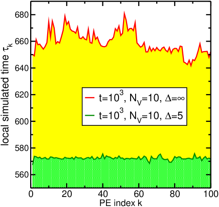
Figure 7: The roughening of the STH. For $\Delta=\infty$ (the upper surface), the crossover time is $t_{\times}\approx 4000$, and for $\Delta=5$ (the lower surface) the width begins to saturate at $t_{p}\approx 40$.

The $\Delta$-constrained time surfaces exhibit the initial growth and the saturation at later times, similar to Fig. 4. However, a detailed analysis of the time evolution of the surface width suggests that, in general, they do not belong to the KPZ universality class unlike surfaces generated with $\Delta=\infty$. Figure 8 presents a typical behavior of the width for $\Delta=10$. In general, the transition to the saturated state takes place over a time interval (a “bump” in Fig. 8), whose length and position depends mainly on the $\Delta$-value and cannot be characterized by a single crossover time. In the initial growth phase for $t\ll t_{p}$ ($t_{p}$ marks the beginning of the plateau, Fig. 8), the surface width scales as $t^{\beta}$, i.e., for a fixed $\Delta$ and $N_{V}$, the growth is characterized by one value of exponent $\beta$ for any $L$. In general, surfaces generated with various values of parameters $\Delta$ and $N_{V}$ are characterized by various effective values of the growth exponent $\beta$. When $\Delta=\infty$, $\beta$ values are between the KPZ value of $1/3$ (for $N_{V}=1$) and the RD value of $1/2$ (for $N_{V}=\infty$) for small and intermediate $N_{V}$ and $L$. In the saturated phase, $t_{p}\ll t$, for a fixed value of $\Delta$, the surface width $\langle w_{L,N_{V}}(t)\rangle$ decreases with the system size, as can be observed from Fig. 8. The saturated surface width as a function of the system size is plotted for $\Delta=100,10,5,1$ in Fig. 9. It can be seen that increasing the number of PEs and the number of sites per PE does not result in infinite roughening of the STH.

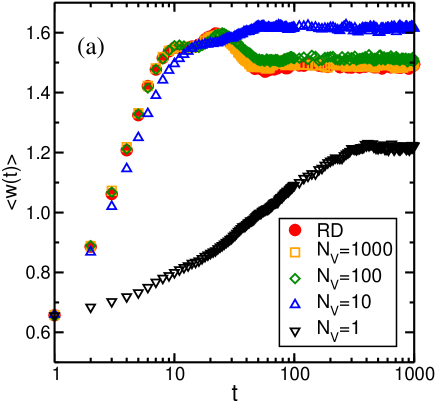
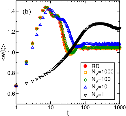
Figure 8: The time evolution of the mean STH surface width $\langle w(t)\rangle$ (averaged over $N=1024$ independent random trials) in PDES with $\Delta=10$, for: (a) $L=100$; (b) $L=1000$. The curves are plotted for several $N_{V}$. Plots of $\langle w_{a}(t)\rangle$ look exactly the same.

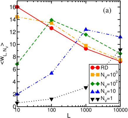
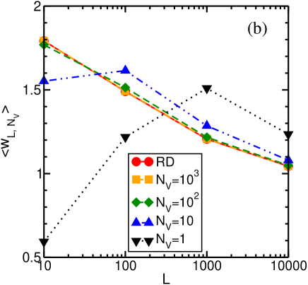
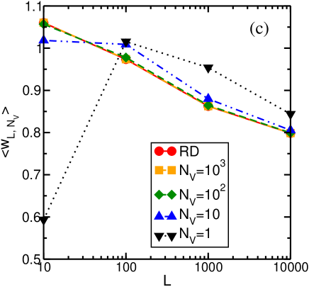
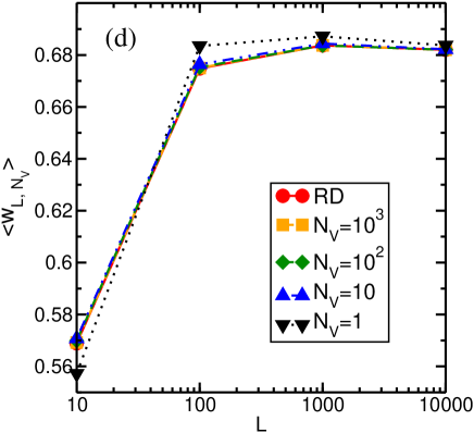
Figure 9: PDES with the $\Delta$-window constraint: The steady state surface width $\langle w\rangle$ of the STH as a function of the system size. (a) $\Delta=100$; (b) $\Delta=10$; (c) $\Delta=5$; and, (d) $\Delta=1$. The curves are plotted for several values of volume elements $N_{V}$. The lines are guides for the eyes.

The STH produced in the RD simulations with the infinite $\Delta$-window (in other words, in PDES with no communication between PEs) is characterized by a surface that is not self-affine BS95 . Nonetheless, the presence of a finite $\Delta$-window constraint in the RD simulations forces the STH surface to saturate (Fig. 8). Therefore, this type of PDES no longer belongs to the RD universality class, characterized by $\beta=0.5$ and $\alpha=\infty$. In the $\Delta$-constrained PDES, the $\Delta$-constrained RD surface is the limiting case when the number of sites per PE grows to infinity.

An interesting feature in the surface width evolution graphs (Fig. 8 and Fig. 10) is the presence of a maximum that marks the end of the growth phase. Its double peak structure can be explained, both quantitatively and qualitatively, in terms of simplex geometry Alfs71 . In the set of $L$ processing elements we distinguish between slow PEs (group (S)) and fast PEs (group (F)). At the $t$-th update attempt, the $k$-th processor belongs to group (S) if its local time ${\tau_{k}}(t)$ is less then or equal to the mean local time over all processors at the $t$-step. Otherwise, it belongs to group (F). One can define the variance $w^{2}$ and the width $w_{a}$ for each group as follows:

$$w_{(X)}^{2}(t)=\frac{1}{{L_{(X)}}(t)}\sum_{k=1}^{L_{(X)}(t)}\left({\tau_{k(X)}}(t)-\bar{\tau}(t)\right)^{2},$$ (15)

$$w_{a(X)}(t)=\frac{1}{{L_{(X)}}(t)}\sum_{k=1}^{L_{(X)}(t)}\left|{\tau_{k(X)}}(t)-\bar{\tau}(t)\right|,$$ (16)

where “X” stands for either “S” or “F”, and $L=L_{(S)}(t)+L_{(F)}(t)$. The variance $w^{2}$ and width $w_{a}$ of the STH can be expressed as the convex linear combinations:

$$w^{2}(t)=f_{(S)}(t)w_{(S)}^{2}(t)+f_{(F)}(t)w_{(F)}^{2}(t),$$ (17)

$$w_{a}(t)=f_{(S)}(t)w_{a(S)}(t)+f_{(F)}(t)w_{a(F)}(t),$$ (18)

where $1=f_{(S)}(t)+f_{(F)}(t)$, $0\leq f_{(S)},f_{(F)}\leq 1$. Explicitly, $w^{2}$ and $w_{a}$ form a 1-d simplex with vertices at S and F. The coefficients $f_{(S)}$ and $f_{(F)}$ are the fractions of slow and fast processors, respectively, in the system at each update attempt $t$. Figure 10 shows the time evolution of the surface widths $w_{a(S)}$, $w_{a(F)}$ and $w_{a}$ (Fig. 10a) and the corresponding fractional contributions $f_{(S)}$ and $f_{(F)}$ (Fig. 10b) for the first $500$ simulation steps. Quantitatively, the double peak in ${w_{a}}(t)$ (at about $t=10$) presents the weighted sum of $w_{a(S)}$ and $w_{a(F)}$ in accordance with Eq. (18), which is evident by matching the width contributions (Fig. 10a) with the corresponding fractional contributions (Fig. 10b) at each $t$-step. Qualitatively, the decrease in surface widths for $t>10$ is the effect of the constraint condition (3). In the particular case of simulations with $\Delta=10$ and $N_{V}=1000$, illustrated in Fig. 10, initially the majority of PEs belongs to the slow group (about $63\%$ at $t=1$, Fig. 10b), but as $t$ advances the STH roughens and the population of the slow group falls while the population in the fast group grows. As the population of the fast group gets larger, the fraction $u$ of PEs that are allowed to update falls because some of the fast PEs violate condition (3). While the fast PEs are waiting (i.e., no local time increments at the fast sites), the slow PEs are incrementing their local times, hence, the mean simulated time increases and therefore the deviation from the mean in Eq. (16) (and Eq.  (15)) decreases for the fast PEs. This is the main mechanism in the formation of the maximum in the $w_{a(F)}$ curve. Similarly, the first maximum in the $w_{a(S)}$ curve is formed mainly due to the depopulation of the slow group. As the slow PEs are “catching up” with the fast PEs within the $\Delta$-window for the update, the utilization $u$ increases ($20<t<50$, Fig. 10b) and so do the widths. This secondary maximum is less pronounced because the populations of the two groups are close apart. Eventually, after several cycles, the widths as well as the utilization reach steady values.

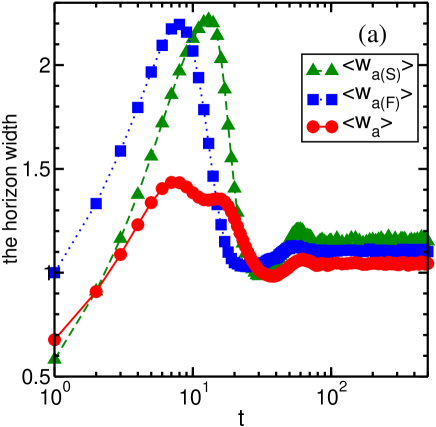
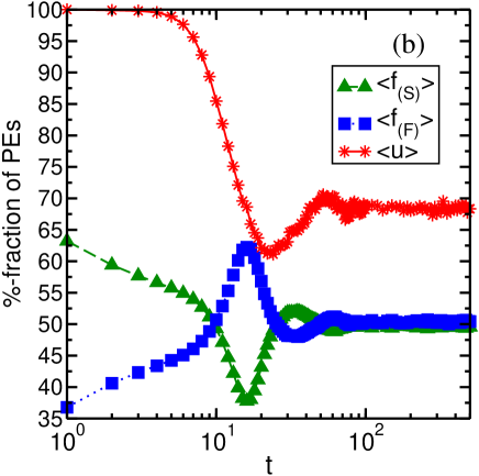
Figure 10: PDES with $\Delta=10$, $N_{V}=10^{3}$ and $L=10^{4}$: (a) Time evolution of the surface widths; (b) Time evolution of $\%$-fractional contributions to the surface widths. Subscripts (S) and (F) denote a fraction of processors in the slow and in the fast group, respectively; and $u$ is the utilization. Configurational averages were taken over $N=1024$ independent random trials. The lines are guides for the eyes.

In other words, the way in which the system undergoes the transition from the initial state to the steady state, observed in the above example, is a direct consequence of the window constrained update scheme (3) and the particular initial condition, in which all PEs enter simulation with their local times equal. If this initial condition of the full synchronization is changed, for example, by assuming that at $t=0$ the local times are randomly distributed about some mean local time, the transition to the steady state will change its character. On the other hand, if at some later update attempt $t_{s}$ the system is synchronized (which is equivalent to setting all local simulated times to one value at $t_{s}$) then the recurrent time evolution will be repeated after $t_{s}$ until the steady state is attained.

The above arguments can be restated in terms of the STH variance $w^{2}$ (taking Eq. (17) as the key to the analysis) for any system size. In the conservative PDES with a moving window constraint the system evolution towards a steady state follows essentially one path, along the above outline, for any value of the simulation parameters $\Delta$, $N_{V}$ and $L$. In our example we chose tentatively a very narrow $\Delta$-window and a large $N_{V}$ so the effect of the update scheme (3) is clearly pronounced in the evolution curves. In such a system,the correlations that arise due to the short-range connection update scheme (1) are small relative to the correlations that arise due to the window constraint (3). Accordingly, in this case one can clearly deduce that a sharp fall in the utilization curve is the effect of a sharp population rise in the group of fast PEs. For example, one can read from Fig. 10b that at $t=10$ about $25\%$ of the PEs that did not make an update were mostly in the group of fast PEs, so approximately about one half of the fast PEs updated at this update attempt. A similar conclusion is certainly false when each PE in the system carries a small number of sites (e.g., $N_{V}=10$) since in this case the correlations that originate due to the short-range connections between PEs may not be neglected and the utilization curve begins the fall at $t=0$ because the fast PEs and the slow PEs fail to satisfy condition (1) with approximately equal frequency. Opening the $\Delta$-window wide (e.g., $\Delta=100$) effects the evolution curves in two ways. First, it slows down the build-up of the correlations that arise due to constraint (3). This makes the growth phase longer so that a transition to the steady state takes place at later times and over extended time intervals. Secondly, it softens the correlations that arise due to constraint (3), which smooths a transition to the steady state and the ripple-like features in the utilization and the width curves (that are clear in Fig. 10) are only weakly present or vanish into statistical uncertainties. For example, in the worst case scenario of $N_{V}=1$ and $\Delta=100$, the time evolution towards the steady state follows the pattern typical for the KPZ universality class ($\Delta=\infty$), which suggests that the main correlation mechanism results from the update scheme (1) in this case. Nonetheless, unlike the KPZ surfaces, the presence of the $\Delta$-window prohibits the steady-state surface width to grow infinitely as the system gets larger.

V DISCUSSION

Our statistical analysis of the growing virtual time interface in conservative asynchronous PDES with a moving window constraint, shows that in the steady state the average utilization remains finite (and non zero) and scales with the system size. Similarly, the statistical spread of the STH remains finite and scales with the system size. This was demonstrated for a range of volume elements from $N_{V}=1$ to the RD-limit at $N_{V}=\infty$. The convergence of the utilization to a finite value and the convergence of the time interface width to a finite value as the number of processing elements infinitely increases, reflects positively on the ability to efficiently implement this type of PDES in applications. In other words, with this global $\Delta$-window constraint the simulation part as well as the measurement part of the algorithm are simultaneously scalable.

The practical questions that should be addressed involve suitable implementations of the algorithm, possible modifications and generalizations that would facilitate applications by optimizing performance and thus maximizing efficiency. Such questions would likely be non-universal, and hence depend on the explicit problem being simulated.

It follows from our analysis that the utilization as defined by a fraction of working processors, is not a sole measure of the efficiency. However, it is an important component of the efficiency. The case of PDES with the basic conservative scheme, when the measurement phase is not scalable, suggests other important factors that should be considered in efficiency studies. The second important component is the statistical spread of the virtual time surface as it is measured by its variance or by its mean absolute deviation. The third important element is the frequency and the effect of extreme fluctuations in the virtual time interface. The forth important factor is the average progress rate, which could be measured by the growth rate of the global minimum of the virtual time interface. An efficient algorithm should be characterized by the highest values of the utilization and the progress rate, while having small statistical spread in waiting times and should lack severe effects of the extreme time fluctuations.

Applying the above recipe to conservative asynchronous PDES with a $\Delta$-window constraint, the results of our studies indicate that this kind of simulation presents a promise of becoming a good departure point towards the design of an efficient class of algorithms for asynchronous systems. The $\Delta$-window constraint not only eliminates the extreme fluctuations in the virtual time horizon but also controls the statistical spread of the STH and controls the average progress rate. The width of the $\Delta$-window can serve as a tuning parameter that, for a given volume load per processor, could be adjusted to optimize the utilization so as to maximize the efficiency.

In the conservative asynchronous PDES studied in this work, there is no condition imposed that would explicitly synchronize a system in the course of the simulations. The system is fully synchronized only initially and undergoes desynchronization over time (i.e., over many parallel steps). The degree of this desynchronization is strictly related to the roughening of the STH. As the simulations evolve, correlations between system components build up, which is reflected by changes in the morphology of the STH. There are two sources of correlations in the STH. The first is the nearest-neighbor communication rule that, if acted alone, would eventually lead to the steady state, where the entire system is correlated. In the case of one volume element per PE, the time to the global correlation is on the order of $L^{3/2}$. However, the presence of this global correlation does not cause an implicit synchronization nor does it lead to a state of near-synchronization. On the contrary, despite this correlation there are no global bounds on the roughening of the virtual time horizon: the larger the system, the more desynchronized it becomes over time. The nearest-neighbor communication rule is the essence of the conservative scheme because it ensures that causality is not violated in any update. The second source of correlations is the constraint in the form of the moving window condition. The moving window condition, if acted alone, would lead to the steady state, where the entire system is not only correlated but, also, is synchronized to some extent. The extent to which the system may become synchronized depends on the width of the moving window — the roughening of the virtual time horizon is constrained to the $\Delta$-window width. Notice, the moving window condition is not necessary for the conservative scheme. Its role is to ensure that infinitely large desynchronization will not happen. In this sense the constraint condition can be seen as an implicit synchronization protocol. In the constrained conservative PDES, the above two correlation mechanisms act together: the nearest neighbor connection rule explicitly guarantees causality and the constraint rule implicitly guarantees a near-synchronization in an arbitrarily long sequence of update attempts.

VI SUMMARY AND OUTLOOK

We considered the conservative parallel discrete event simulations with the moving window constraint and studied the time evolution of the utilization as well as the time evolution of the stochastic time horizon by varying the system size (i.e., the number $L$ of processing elements and the number $N_{V}$ of sites per processing element) and by varying the width of the moving window. The results of our simulations indicate that this particular class of algorithms with the conservative update scheme generally scales with the system size. The utilization reaches a steady state value after a finite number of simultaneously performed parallel steps and approaches a finite non-zero value in the limit of infinite system size. This demonstrates that the simulation part of the algorithm is scalable. The statistical spread of the stochastic time horizon is bounded by the size of the moving window constraint in the limit of the infinite system size, which shows that the measurement part of the algorithm is scalable. In particular, in the limit of a large number of sites per processing element the results of the simulations approach the constrained random deposition model, which is characterized by a high value of utilization while permitting effective data management. The simultaneous scalability of both phases of the algorithm is an important finding because it establishes a solid ground for the design of new class of efficient algorithms for parallel processing to model the evolution of spatially extended interacting systems with asynchronous dynamics. Further studies are required in the search for possible optimal implementations. For example, explicitly taking into account the time required to find the global minimum of the STH at each step.

Aside from practical aspects of the constrained parallel conservative discrete event simulations that are oriented to direct applications such as the scalability issues, there are several interesting physics questions that arise in connection with the stochastic time surface growth. These include the development of the lateral correlations and transient relaxation processes. We leave these questions open to possible future investigations.

*

Appendix A The utilization data

In the infinite $L$-limit the utilization is a two parameter family of curves (Fig. 6). The two limiting curves, $u_{RD}(\Delta)$ and $u_{KPZ}(N_{V})$, approach $u=1$ in the infinite limit of their arguments. One can consider either $u_{RD}$ or $u_{KPZ}$ as an independent variable $x$ and express the utilization as $y=y(x)$. We chose parameterization by $N_{V}$, where $x=x(N_{V})=u_{KPZ}(N_{V})$ and $y_{\Delta}(x)=y_{\Delta}\left(x(N_{V})\right)$. Figure 11 illustrates the idea by plotting the utilization $y_{\Delta}(x)$ for several values of $\Delta$. The curves in Fig. 11 are a family of roots that, in first approximation, could be expressed by $y_{\Delta}(x)=a(\Delta)x^{p(\Delta)}$, where $a(\Delta)$ and $p(\Delta)$ have fractional values. To find $a(\Delta)$ and $p(\Delta)$ each curve is fitted to “the best” two-point formula. Then, sequences $a(\Delta)$ and $p(\Delta)$ are expressed by fit functions.

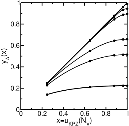
Figure 11: Family of utilization curves $y_{\Delta}(x)$ vs $x=u_{KPZ}(N_{V})$, illustrating the underlying idea of the fit. For $\Delta_{1}<\Delta_{2}<\dots<\Delta=\infty$, $y_{\Delta_{1}}<y_{\Delta_{2}}<\dots<y_{\infty}=x$. For $\Delta=0$, $y_{\Delta}(x)=0$ (not shown). Symbols mark the simulation data. The cubic spline curves are guides for the eyes.

A fit to $a(\Delta)$ is chosen in such a way that $a(0)=0$ and $a(\infty)=1$. In Fig. 11, $a(0)=0$ corresponds to $y(x)=0$ because $\Delta=0$ yields $u\equiv 0$ for $L=\infty$. Condition $a(\infty)=1$ corresponds to $y(x)=x$ because $\Delta=\infty$ means $y=u_{KPZ}$. Considering the limit behavior of $y_{\Delta}(x)$, when $x(N_{V}=\infty)=1$ the coefficient $a(\Delta)$ must be interpreted as $u_{RD}(\Delta)$. This is also consistent with the alternative parameterization, where $x=u_{RD}(\Delta)$. Therefore, we directly identify $a(\Delta)$ with the approximate expression for $u_{RD}(\Delta)$. A four-point fit can be found as:

$$u_{RD}(\Delta)\approx a(\Delta)\cong\frac{1}{\displaystyle 1+\frac{c_{3}}{\Delta^{e_{3}}}-\frac{c_{4}}{\Delta^{e_{4}}}}.$$ (19)

When $c_{3}=15.8$, $e_{3}=1.07$, $c_{4}=12.3$ and $e_{4}=1.18$, fit (19) is good within $\pm 2\%$ relative error in the range $0\leq\Delta<\infty$. A simple two-point fit with $c_{3}=3.47$, $e_{3}=0.84$ and $c_{4}=e_{4}=0$ approximates our simulated data within $\pm 2.5\%$ relative difference (Fig. 6, utilization values for $N_{V}=10^{8}$).

Considering the limits $u_{KPZ}(N_{V}=1)\approx 1/4$ and $u_{KPZ}(N_{V}=\infty)=1$, a four-point fit to $x(N_{V})$ is:

$$u_{KPZ}(N_{V})=x(N_{V})\cong\frac{1}{\displaystyle 1+\frac{c_{1}}{N_{V}^{e_{1}}}+\frac{c_{2}}{N_{V}^{e_{2}}}}.$$ (20)

When $c_{1}=2.3$, $e_{1}=0.96$, $c_{2}=0.74$ and $e_{2}=0.4$, fit (20) is good to within $\pm 2\%$ relative error in the range $1\leq N_{V}<\infty$. A simple two-point fit with $c_{1}=3.0$, $e_{1}=0.715$ and $c_{2}=e_{2}=0$ approximates our simulated data within $\pm 2.5\%$ relative difference (Fig. 6, utilization values for $\Delta=\infty$).

In fitting the power $p(\Delta)$, the limits are $p(\Delta=\infty)=1$ and $p(0)=0$. In Fig. 11, condition $p(\Delta=\infty)=1$ means $y(x)=x$. Condition $p(0)=0$ expresses the fact that for small $\Delta$ the utilization depends mainly on $\Delta$ (not $N_{V}$) and, therefore, the exponent $p(\Delta)$ should be almost zero for small $\Delta$. A simple two-point formula gives $p(\Delta)=1/(1+2/{\Delta^{3/4}})$. With this $p(\Delta)$, a simple fit to $u(N_{V},\Delta)\approx a(\Delta)x(N_{V})^{p(\Delta)}$ has a $\pm 10\%$ relative error when $a(\Delta)$ and $x(N_{V})$ are given by simple two-point fits. The actual power $p$ depends weakly also on $N_{V}$, $p=p(\Delta,N_{V})$. A four-point formula that accommodates the $N_{V}$ dependance can be expressed as:

$$p(\Delta,N_{V})\approx\frac{1}{\displaystyle 1+\frac{c_{5}(N_{V})}{\Delta^{e_{5}(N_{V})}}-\frac{c_{6}(N_{V})}{\Delta^{e_{6}(N_{V})}}}.$$ (21)

The fit (12) is good to within $\pm 5\%$ relative uncertainty for all $\Delta$- and $N_{V}$-values when $u_{RD}$ and $u_{KPZ}$ are expressed by four-point fits (19) and (20), respectively, and when $p$ is given by (21) with the following fit parameters: for $N_{V}\geq 100$: $c_{5}=528.4$, $e_{5}=1.487$, $c_{6}=515.1$, $e_{6}=1.609$; for $N_{V}<10$: $c_{5}=17.43$, $e_{5}=1.406$, $c_{6}=15.3$, $e_{6}=1.687$; otherwise: $c_{5}=5.345$, $e_{5}=0.627$, $c_{6}=0.095$, $e_{6}=0.045$.

References

- (1) R. Fujimoto, Commun. of the ACM 33, 30 (1990).
- (2) D.M. Nicol and R.M. Fujimoto, Annals of Operations Research 53, 249 (1994).
- (3) K. Binder and D.W. Heermann, Monte Carlo Simulation in Statistical Physics. An Introduction, 3rd ed. (Springer, Berlin 1997).
- (4) K.M. Chandy and J. Misra, IEEE Trans. on Softw. Eng. SE-5, 440 (1979).
- (5) K.M. Chandy and J. Misra, Commun. ACM 24, 198 (1981).
- (6) B.D. Lubachevsky, Complex Systems 1, 1099 (1987).
- (7) B.D. Lubachevsky, J. Comp. Phys. 75, 103 (1988).
- (8) Blue Gene/L project, partnership between IBM and DoE, announced Nov.9, 2001; expected scale 200 teraflops, a step towards a petaflop scale; expected completion 2005; IBM Research Report, RC22570 (W0209-033) September 10, 2002.
- (9) A.-L. Barabasi and H.E. Stanley, Fractal Concepts in Surface Growth (Cambridge University Press, Cambridge, 1995).
- (10) R.E. Feldman and Kleinrock, ACM Trans. Model. Comput. Simul. 1, 386 (1991).
- (11) D.M. Nicol, ACM Trans. Model. Comput. Simul. 1, 24 (1991).
- (12) J.S. Steiman, in Proceedings of the 7th Workshop on Parallel and Distributed Simulation (PAD’93), Vol. 23, No.1, edited by R. Bagrodia and D. Jefferson (Soc. Comput. Simul., San Diego, CA, 1993).
- (13) J.S. Steiman, in Proceedings of the 8th Workshop on Parallel and Distributed Simulation (PAD’94), edited by D.K Arvind, R. Bagrodia and J. Y.-B. Lin (Soc. Comput. Simul., San Diego, CA, 1994).
- (14) J.S. Steiman, in Proceedings of the 9th Workshop on Parallel and Distributed Simulation (PAD’96), (IEEE Comput. Soc. Press, Los Alamitos, CA, 1996).
- (15) P.M.A. Sloot, B.J. Overeiner, and A. Schoneveld, Comp. Phys. Commun. 142, 76 (2001).
- (16) B.J. Overeiner, A. Schoneveld, and P.M.A. Sloot, in Proceedings of the 15th Workshop on Parallel and Distributed Simulation (PAD’96), (IEEE Comput. Soc. Press, Los Alamitos, CA, 2001).
- (17) G. Korniss, M.A. Novotny, and P.A. Rikvold, Comp. Phys. 153, 488 (1999).
- (18) B.D. Lubachevsky, V.Privman, and S.C. Roy, J. Comp. Phys. 126, 152 (1996).
- (19) G. Korniss, C.J. White, P.A. Rikvold, and M.A. Novotny, Phys. Rev. bf E63, 016120 (2001).
- (20) G. Korniss, P. A. Rikvold, and M. A. Novotny, to appear in Phys. Rev. E (Nov.1, 2002); e-print cond-mat/0207275 (2002).
- (21) B.D. Lubachevsky, in Distributed Simulation 1989, SCS simulation series, Vol.21 (Society of Computer Simulation, San Diego, CA, 1989).
- (22) D.M. Nicol, J. ACM 40, 304 (1993).
- (23) G. Korniss, Z. Toroczkai, M.A. Novotny, and P.A. Rikvold, Phys. Rev. Lett. 84, 1351 (2000).
- (24) G. Korniss, M.A. Novotny, A.K. Kolakowska, and H.Guclu, in Proceedings of the 2002 ACM Symposium on Applied Computing, p.132 (2002).
- (25) G. Korniss, M.A. Novotny, Z. Toroczkai, and P.A. Rikvold, in Computer Simulation Studies in Condensed Matter Physics XIII, edited by D.P. Landau, S.P. Lewis, and H.-B. Shuttler, Springer Proceedings in Physics, Vol.86 (Springer-Verlag, Heidelberg, 2001) p.183.
- (26) G. Korniss, M. A. Novotny, P. A. Rikvold, H. Guclu, and Z. Toroczkai, in Materials Research Society Symposium Proceedings Series, Combinatorial and Artificial Intelligence Methods in Materials Science, Vol. 700, p. 297 (2002).
- (27) A. Greenberg, S. Shenker, and A.L. Stolyar, Proc. ACM SIGMETRICS, Performance Eval. Rev. 24, 91 (1996).
- (28) G. Korniss, M. A. Novotny, H.Guclu, Z. Toroczkai, and P. A. Rikvold, unpublished.
- (29) M. Kardar, G. Parisi, and Y.-C. Zhang, Phys. Rev. Lett. 56, 889 (1986).
- (30) T. Halpin-Healy and Y.-C. Zhang, Phys. Rep. 254, 215 (1995).
- (31) J. Krug, Adv. Phys. 46, 139 (1997).
- (32) J. Krug and P. Meakin, J. Phys. A23, L987 (1990).
- (33) Z. Toroczkai, G. Korniss, S. Das Sarma, and R.K.P. Zia, Phys. Rev. E62, 276 (2000).
- (34) W. H. Press, S. A. Teukolsky, W. T. Vetterling, and B. P. Flannery, Numerical Recipes in Fortran 77 (Cambridge University Press, Cambridge, 1992).
- (35) E. M. Alfsen, Compact Convex Sets and Boundary Integrals (Springer-Verlag, New York, 1971).