Improved Phylogeny Comparisons: Non-Shared Edges, Nearest Neighbor Interchanges, and Subtree Transfers

Abstract

The number of the non-shared edges of two phylogenies is a basic measure of the dissimilarity between the phylogenies. The non-shared edges are also the building block for approximating a more sophisticated metric called the nearest neighbor interchange (NNI) distance. In this paper, we give the first subquadratic-time algorithm for finding the non-shared edges, which are then used to speed up the existing approximating algorithm for the NNI distance from $O(n^{2})$ time to $O(n\log n)$ time. Another popular distance metric for phylogenies is the subtree transfer (STT) distance. Previous work on computing the STT distance considered degree-$3$ trees only. We give an approximation algorithm for the STT distance for degree-$d$ trees with arbitrary $d$ and with generalized STT operations.

1 Introduction

Phylogenies are trees whose leaves are labeled with distinct species. Different theories about the evolutionary relationship of the same species often result in different phylogenies. This paper is concerned with three well-known metrics for measuring the dissimilarity between two phylogenies, namely, the non-shared edge distance [1, 14, 11], the nearest neighbor interchange(NNI) distance [13, 12] and the subtree transfer(STT) distance [7, 8]. The first metric counts the number of edges that differentiate the phylogenies; the other two metrics measure the minimum total cost of some kind of tree operations required to transform one phylogeny to the other. For the NNI distance, an operation swaps two subtrees over an internal edge; for the STT distance, an operation detaches a subtree from a node and re-attaches it to another part of the tree.

In this paper we consider phylogenies of degrees $d$ whose edges may carry weights. Given two weighted degree-$d$ phylogenies $T$ and $T^{\prime}$, an edge $e$ in $T$ is shared if for some edge $e^{\prime}$ in $T^{\prime}$, the removals of $e$ and $e^{\prime}$ from $T$ and $T^{\prime}$, respectively induce the same partition of leaf labels, internal node degrees, and edge weights; otherwise, $e$ is non-shared. Previously, non-shared edges could be found using a brute-force approach in $O(n^{2})$ time, where $n$ is the number of leaves. If we restrict our attention to the partition of leaf labels only, Day [4] reduced the time to $O(n)$. We give an $O(n\log n)$-time algorithm for finding the general non-shared edges.

Finding non-shared edges is a key step, as well as the most time consuming step, for approximating the NNI distance. In particular, for degree-3 phylogenies with weights or degree-$d$ phylogenies with or without weights, existing approximation algorithms take $O(n^{2})$ time [3, 10]. With our new non-shared edge algorithm, the time complexity of these approximation algorithms can all be improved to $O(n\log n)$. Note that for unweighted degree-3 trees, an $O(n\log n)$-time algorithm has already been obtained [11], which uses Day’s linear-time algorithm [4] to identify the non-shared edges.

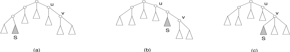
Figure 1: Examples of restricted-STT and STT operations. Tree (a) is transformed to tree (b) by a restricted-STT operation, while tree(a) is transformed to tree (c) by an STT operation.

Previous work on STT distance focuses on degree-3 trees only [9, 2]. In particular, in the course of transforming a degree-3 tree to another degree-3 tree, all intermediate trees are required to be of degree 3. In other words, the STT operation is restricted in the sense that the subtree detached can only be re-attached to the middle of an edge, producing a new internal node with degree 3. See Figure 1 for an example. In this paper we study the STT distance for degree-$d$ phylogenies for any $d\geq 3$ while also allowing an STT operation to re-attach the subtree to either an internal node or the middle of an edge.

An STT operation is charged by how far a subtree is transferred. More specifically, depending on whether the trees are unweighted or weighted, we count respectively the number of the edges or the total weight of the edges between the nodes where detachment and re-attachment take place. We formally define the STT (respectively, restricted-STT) distance between two phylogenies as the minimum cost of transforming one to the other using STT (respectively, restricted-STT) operations. Unlike many other graph or tree problems, the unweighted version of the STT distance problem is not a special case of the weighted version. In particular, Figure 2 shows two phylogenies whose unweighted STT distance is $\Omega(n)$, yet if we assign a unit weight to every edge of these phylogenies, their weighted STT distance is only $O(1)$. On the other hand, the unweighted STT distance is not necessarily bigger than the weighted one; Figure 3 shows two phylogenies whose unweighted STT distance is indeed smaller than the weighted one.

Figure 2: The unweighted STT distance between $T$ and $T^{\prime}$ is $\Omega(n)$. Consider $T$ and $T^{\prime}$ as weighted trees such that every internal edge has a unit weight (i.e., the highlighted edges in the figure). The weighted STT distance between $T$ and $T^{\prime}$ is 1. In particular, the cost of transforming $T$ to $R$, then to $R^{\prime}$, and finally to $T^{\prime}$ is $0+1+0=1$.

Figure 3: $T$ and $T^{\prime}$ are degree-3 phylogenies. The unweighted STT distance between $T$ and $T^{\prime}$ (which is 3) is smaller than the weighted STT distance (which is 4).

Consider degree-3 phylogenies. In the weighted case, we can prove that the STT distance is the same as the restricted-STT distance, and DasGupta et al. have shown that the latter can be approximated within a factor of 2 [2]. In the unweighted case, deriving a tight approximation algorithm is more difficult; the restricted-STT distance can be approximated within only a factor of $O(\log n)$ [2]. This result implies an approximation algorithm for the STT distance with the same performance. However, there are examples in which the STT distance is much smaller than the restricted-STT distance. It is natural to ask whether the STT distance can be approximated within a better factor.

Consider degree-$d$ phylogenies. First of all, it is worth mentioning that the restricted-STT distance is $\infty$ as a restricted-STT operation can only produce an internal node of degree 3. In the weighted case, the STT distance can be approximated by adapting the algorithm by DasGupta et al for degree-3 trees [2], achieving the approximation factor of 2. In the unweighted case, we give an algorithm to approximate the STT distance within a factor of $2d-4$. This result implies that for unweighted degree-3 trees, the approximation factor can be improved from $O(\log n)$ to $2$ if the intermediate trees may not be necessarily degree-$3$ trees. Table 1 summarizes the approximation factors for the variants of the STT distance.

Table 1: The approximation factors for the different variants of the STT distance.

	restricted-STT	STT
	(degree-3 trees)	(degree-$d$ trees)
weighted	2 [2]	2
unweighted	$O(\log n)$ [2]	$2d-4$

The following summarizes the contributions of the paper.

1. We give the first subquadratic (i.e., $O(n\log n)$) time algorithm for finding the non-shared edges between two weighted phylogenies, thus improving the time complexity of the algorithms in [3, 10] for approximating the NNI distance from $O(n^{2})$ to $O(n\log n)$.

2. We show that the problem of finding the STT distance between two weighted degree-$d$ phylogenies is equivalent to the problem of finding the restricted-STT distance between two weighted degree-3 phylogenies. This result implies the following.

   1. The STT distance between two weighted degree-$d$ phylogenies can be approximated within a factor of 2.

   2. If the leaf labels of the trees are not distinct, it is NP-hard to compute the STT distance between two trees.

3. We give an approximation algorithm with approximation ratio of $2d-4$ for finding the STT distance between two unweighted degree-$d$ phylogenies.

4. We prove that it is NP-hard to compute the STT distance between two unweighted trees with leaves labeled by possibly non-distinct labels.

The rest of this paper is organized as follows. Section 2 gives the $O(n\log n)$-time algorithm for finding the non-shared edges between two weighted trees. Section 3 presents the results on computing subtree transfer distance for both weighted and unweighted cases. Finally, Section 4 shows that computing STT distance between two unweighted phylogenies with possibly non-distinct labels is NP-hard.

2 Finding non-shared edges between weighted trees

In this section, we show how to find all non-shared edges between two weighted phylogenies in $O(n\log n)$ time. Basically, we tranform the problem to a partition labeling problem which can be solved in $O(n\log n)$ time. In Section 2.1, we define the partition labeling problem on two rooted trees and solve the problem in $O(n\log n)$ time. In Section 2.2, we define the non-shared edge problem and give an $O(n\log n)$-time reduction from the non-shared edge problem to the partition labeling problem.

The following multi-set notations are used in this section. Let $M=\{a,a,\dots,b,b,\dots\}$ be a multi-set of symbols. Let $\delta(M)$ be the set of distinct symbols in $M$. For each $a\in\delta(M)$, let $\#a$ be the number of occurrences of $a$ in $M$. Let $|M|=\sum_{a\in\delta(M)}{\#a}$. Furthermore, the set operations for any two multi-sets $M$ and $N$ are defined as follows: (i) $M\subseteq N$ if for each $a\in\delta(M)$, $\#a$ in $M\leq\#a$ in $N$. (ii) $M=N$ if $M\subseteq N$ and $N\subseteq M$. (iii) $M\cup N$ is defined to be a multi-set containing $\max\{\#a\mbox{~{}in~{}}M,\#a\mbox{~{}in~{}}N\}$ copies of $a$ for each $a$ in $\delta(M)\cup\delta(N)$.

2.1 The partition labeling problem for rooted trees

In this section we define the partition labeling problem for two rooted trees with leaves labeled by the same multi-set of labels and solve the problem in $O(n\log n)$ time, where $n$ is the number of leaves in either tree. In the following, let $R$ and $R^{\prime}$ be two rooted trees with leaves labeled by the same multi-set $S$ of labels, and let $A$ be any subset of $\delta(S)$.

For each internal node $u$ in $R$, we define the following.

• Let $L_{R}(u)$ be the multi-set of leaf labels in the subtree of $R$ rooted at $u$.

• Let $L_{R}(u)|A$ be the multi-set of leaf labels constructed from $L_{R}(u)$ by deleting all labels which are not in $A$.

Given $R$ and $R^{\prime}$, let $V$ be the union of the sets of internal nodes in $R$ and $R^{\prime}$. A mapping $\rho:V\rightarrow[1..t]$ (where $t=|V|$) is called a partition labeling for $R$ and $R^{\prime}$ if for any $u$ in $R$ and $v$ in $R^{\prime}$, $\rho(u)=\rho(v)$ if and only if $L_{R}(u)=L_{R^{\prime}}(v)$.

The partition labeling problem is to find a partition labeling for $R$ and $R^{\prime}$. Note that this partition labeling always exists. A straightforward approach is to compute all multi-sets of $L_{R}(u)$ (and $L_{R^{\prime}}(v)$) first and then assign a unique integer to each distinct multi-set. However, each multi-set can be as large as $O(n)$, so this straightforward approach takes $O(n^{2})$ time.

To reduce the time complexity, we compute the multi-sets in an incremental manner, and start comparing them earlier based on the partial result. In particular, we assign a temporary label to represent each multi-set, such that two multi-sets are assigned the same label if they are equal. This helps in saving not only the space for storing the multi-sets, but also the time for comparing two multi-sets afterwards. The labels will further be updated by a relabeling process, as long as more information about the multi-sets are computed. In the end, each distinct multi-set of $L_{R}(u)$ (and $L_{R^{\prime}}(u)$) obtains a distinct label.

The algorithm is presented in Figure 4, where $R_{A}$ is defined as the subtree of $R$ induced by $A$. Precisely, $R_{A}$ is a tree constructed by contracting $R$ to retain only those leaves with labels in $A$ and their least common ancestors.

The algorithm is analysed below, and we begin with two supporting lemmas.

Phase 1. For each label $i$ in $\delta(S)$, find a parition labeling for $R_{\{i\}}$ and $R^{\prime}_{\{i\}}$ according to Lemma 2.3. Phase 2. Repeat the following procedure for $\log|\delta(S)|$ rounds:
Let $A_{1},A_{2},\ldots$ be the sets of labels considered in the last step. 1. Pair up $A_{i}$’s such that $A_{2j-1}=A_{2j-1}\cup A_{2j}$. 2. Delete all $A_{2j}$’s and rename $A_{2j-1}$ as $A_{j}$. 3. For each $A_{j}$, compute a partition labeling for $R_{A_{j}}$ and $R^{\prime}_{A_{j}}$ based on the result of the last step and Lemma 2.4.

Figure 4: Partition labeling for $R$ and $R^{\prime}$.

Lemma 2.1

The induced subtree $R_{A}$ can be constructed in $O(t)$ time where $t$ is the number of leaves in $R$ with labels in $A$.

Proof.

Using the algorithm in [6], with linear time preprocessing, we can answer a least common ancestor query in constant time. To construct $R_{A}$, we only need to answer $O(t)$ least common ancestor queries where $t$ is the number of leaves in $R$ with labels in $A$, so the lemma follows. ∎

Lemma 2.2

Let $A$ and $B$ be two disjoint subsets of $\delta(S)$. Let $u$ be an internal node in $R_{A\cup B}$. Then $L_{R_{A\cup B}}(u)|A=\emptyset$ or $L_{R_{A}}(v)$ for some $v$ in $R_{A}$. (Similarily, $L_{R_{A\cup B}}(u)|B=\emptyset$ or $L_{R_{B}}(v)$ for some $v$ in $R_{B}$.)

Proof.

If $u$ is in $R_{A}$, $L_{R_{A\cup B}}(u)|A=L_{R_{A}}(u)$. It remains to consider $u$ not in $R_{A}$. Suppose on the contrary that $L_{R_{A\cup B}}(u)|A\neq\emptyset$ and $L_{R_{A\cup B}}(u)|A\neq L_{R_{A}}(v)$ for any internal node $v$ in $R_{A}$. Let this $u$ be the first one of this kind visited by a postorder traversal of $R_{A\cup B}$.

By the construction of $R_{A}$, since $u$ is not in $R_{A}$, $u$ has at most one child $s$ whose subtree contains leaf labels in $A$. If such an $s$ exists, then $L_{R_{A\cup B}}(u)|A=L_{R_{A\cup B}}(s)|A$. This contradicts the choice of $u$. If $u$ has no such a child, $L_{R_{A\cup B}}(u)|A=\emptyset$. Thus such a $u$ does not exist. A similar argument can be applied to the case of $L_{R_{A\cup B}}|B$. ∎

The next lemma implies that Phase 1 can be computed in $O(n)$ time.

Lemma 2.3

Let $a\in\delta(S)$. A partition labeling for $R_{\{a\}}$ and $R^{\prime}_{\{a\}}$ can be found in $O(t)$ time where $t$ is the number of leaves in $R$ with label $a$.

Proof.

Perform a postorder traversal in $R_{\{a\}}$. Since $L_{R_{\{a\}}}(u)$ only contains multiple copies of $a$, we only need to keep track $|L_{R_{\{a\}}}(u)|$ during the traversal and assign this number to the internal node $u$. Apply the same procedure to $R^{\prime}_{\{a\}}$. ∎

After Phase 1, we get the partition labeling for $R_{\{i\}}$ for every label $i\in\delta(S)$. Phase 2 tries to merge the $R_{\{i\}}$’s incrementally until we get the partition labeling for $R_{\delta(S)}$. Below we describe the merging process. Let $A$ and $B$ be two disjoint subsets of $\delta(S)$. Let $\rho_{1}$ and $\rho_{2}$ be partition labelings for $(R_{A},R_{A}^{\prime})$ and $(R_{B},R_{B}^{\prime})$, respectively. Now, we perform the following relabeling process on the internal nodes of $R_{A\cup B}$ and $R^{\prime}_{A\cup B}$.

Relabeling Process: Consider $R_{A\cup B}$ (similar for $R^{\prime}_{A\cup B}$).

Step 1.

Perform a postorder traversal. For each internal node $u$ in $R_{A\cup B}$ visited, assign a 2-tuple of integers $(a,b)$ to $u$ in the following manner:
According to Lemma 2.2, if $L_{R_{A\cup B}}|A=\emptyset$, set $a$ to 0; Otherwise, there exists a $v$ such that $L_{R_{A\cup B}}|A=L_{R_{A}}(v)$, then set $a$ to $\rho_{1}(v)$. Set $b$ similarily by considering $L_{R_{A\cup B}}|B$.

Step 2.

Sort all 2-tuples of internal nodes by radix sort. Traverse the sorted list of these 2-tuples, assign a new integer (starting from 1) to every distinct 2-tuple encountered. Assign this integer as a label to the corresponding internal node.

In fact, the labels assigned to the nodes in the relabeling process form a valid partition labeling. We have the following lemma.

Lemma 2.4

Given the partition labelings for $(R_{A},R_{A}^{\prime})$ and $(R_{B},R_{B}^{\prime})$, we can compute a partition labeling for $R_{A\cup B}$ and $R^{\prime}_{A\cup B}$ in $O(t)$ time where $t$ is the number of leaves in $R_{A\cup B}$.

Proof.

Perform the relabeling process on $R_{A\cup B}$. Since $L_{R_{A\cup B}}(u)=L_{R_{A\cup B}}(u)|A\cup L_{R_{A\cup B}}(u)|B$, $L_{R_{A\cup B}}(p)=L_{R^{\prime}_{A\cup B}}(q)$ if and only if the corresponding 2-tuples assigned to $p$ and $q$ are identical. So, the labels assigned to the nodes in Step 2 form a valid parition labeling.

Regarding the time complexity, in Step 1, during the postorder traversal, for each internal node $u$, if $u$ is in $R_{A}$, then $v=u$. Otherwise, if there exists a child $s$ of $u$ in $R_{A\cup B}$ with $L_{R_{A\cup B}}(s)|A=L_{R_{A}}(t)$, then $v=t$. If no such $s$ exists, $L_{R_{A\cup B}}(u)|A=\emptyset$. So, this Step can be completed in linear time. Obviously, Step 2 can also be completed in linear time, so the lemma follows. ∎

Lemma 2.4 implies that each round of Phase 2 takes $O(n)$ time. This gives the following lemma.

Lemma 2.5

Given $R$ and $R^{\prime}$, a partition labeling for $R$ and $R^{\prime}$ can be computed in $O(n\log n)$ time where $n$ is the number of leaves in $R$.

Proof.

By Lemma 2.3, Phase 1 takes $O(n)$ time. By Lemma 2.4, each round in Phase 2 takes $O(n)$ time, so the overall complexity is $O(n\log|\delta(S)|)=O(n\log n)$ time. Thus, the lemma follows. ∎

2.2 An $O(n\log n)$-time algorithm for finding non-shared edges

In this section we show that the non-shared edge problem for weighted phylogenies can be solved by an $O(n\log n)$-time reduction to the partition labeling problem on two rooted trees.

Let $T$ and $T^{\prime}$ be two weighted phylogenies with the same set of distinct leaf labels and the same multi-set of edge weights and internal node degrees. Recall that a shared edge is defined as follows.

An edge $e$ in $T$ is said to be shared (with respect to $T^{\prime}$) if there exists an edge $e^{\prime}$ in $T^{\prime}$ such that $e$ and $e^{\prime}$ induce the same partition of leaf labels, internal node degrees, and edge weights in $T$ and $T^{\prime}$, respectively; otherwise, $e$ is non-shared.

The non-shared edge problem is to find all non-shared edges in $T$ (with respect to $T^{\prime}$) and all non-shared edges in $T^{\prime}$ (with respect to $T$). Figure 5 gives the details of the reduction from the non-shared edge problem to the partition labeling problem. Basically, edge weights and node degrees in $T$ and $T^{\prime}$ will be represented by new labeled leaves in the two constructed trees $R$ and $R^{\prime}$, respectively.

1. Set $R=T$ and $R^{\prime}=T^{\prime}$. 2. Fix an arbitrary leaf with label $a$. Root $R$ and $R^{\prime}$ at the internal nodes which attach to leaves with label $a$. 3. Attach a new leaf to every internal node of $R$ and $R^{\prime}$ such that the labels of such new leaves are the same if the corresponding internal nodes have the same degree. 4. Attach a new leaf in the middle of every internal edge in both $R$ and $R^{\prime}$ such that the labels of such new leaves are the same if the original edges have the same weight.

Figure 5: Construction of $R$ and $R^{\prime}$ from $T$ and $T^{\prime}$.

Note that $R$ and $R^{\prime}$ have the same multi-set of leaf labels since $T$ and $T^{\prime}$ have the same multi-set of leaf labels, edge weights, and node degrees. And the number of leaves in $R$ and $R^{\prime}$ is of $O(n)$ where $n$ is the number of leaves in $T$.

Lemma 2.6

The construction of $R$ and $R^{\prime}$ takes $O(n\log n)$ time.

Proof.

The lemma follows since Step 4 takes at most $O(n\log n)$ time, Step 3 takes $O(n)$ time, and Steps 1 and 2 take $O(1)$ time. ∎

The following lemma relates the non-shared edges problem and the partition labeling problem.

Lemma 2.7

Given a partition labeling $\rho$ for $R$ and $R^{\prime}$, let $(u,v)$ be an edge in $T$ and $s$ be the unique internal node between $u$ and $v$ in $R$. Then, the edge $(u,v)$ is a non-shared edge in $T$ (w.r.t. $T^{\prime}$) if and only if the label $\rho(s)$ is unique in $\rho$.

Proof.

Suppose that $(u,v)$ is a non-shared edge in $T$. By the construction of $R$ and $R^{\prime}$, $L_{R}(s)$ must be unique. So, $\rho(s)$ is unique in $\rho$.

On the other hand, if $(u,v)$ is a shared-edge in $T$, then there is another edge $(u^{\prime},v^{\prime})$ in $T^{\prime}$ such that $(u,v)$ and $(u^{\prime},v^{\prime})$ induce the same partition of leaf labels, node degrees, and edge weights in $T$ and $T^{\prime}$, respectively. Without loss of generality, let $u$ and $u^{\prime}$ be the portion containing the leaf with label $a$. Then, $u$ and $u^{\prime}$ are the ancestors of $v$ and $v^{\prime}$ in $R$ and $R^{\prime}$ respectively. Let $s^{\prime}$ be the unique internal node between $u^{\prime}$ and $v^{\prime}$. By the construction of $R$ and $R^{\prime}$, $L_{R}(s)=L_{R^{\prime}}(s^{\prime})$. ∎

In conclusion, we have the following theorem.

Theorem 2.8

The non-shared edges of $T$ and $T^{\prime}$ can be identified in $O(n\log n)$ time.

Proof.

By Lemma 2.7, if a partition labeling for $R$ and $R^{\prime}$ is given, we can identify all non-shared edges in $T$ and $T^{\prime}$ in $O(n)$ time. Since the parition labeling problem can be solved in $O(n\log n)$ time, the theorem follows. ∎

3 The STT distance between degree-$d$ phylogenies

This section studies the problem of computing the STT distance between two degree-$d$ phylogenies in both weighted and unweighted cases. For the weighted case, we show that the problem of computing the STT distance between two weighted degree-$d$ phylogenies (the weighted STT-d problem) is equivalent to the problem of computing the restricted-STT distance between two weighted degree-$3$ phylogenies (the weighted rSTT-3 problem). Since DasGupta et al [2] have shown that the weighted rSTT-3 problem is NP-hard and can be approximated within a factor of 2, the same results apply to the weighted STT-$d$ problem. For the unweighted case, we give a new approximation algorithm with an approximation factor of $2d-4$ for finding the STT distance between two degree-$d$ phylogenies (the unweighted STT-d problem). We also prove that the problem of computing the STT distance between two unweighted phylogenies with possibly non-distinct labels is NP-hard.

Section 3.1 gives notations and defintions used in this section. Section 3.2 gives the result for the weighted case. Section 3.3 gives an approximation algorithm for computing the STT distance between two unweighted phylogenies. Section 4 shows that it is NP-pard to compute STT distance between two unweighted phylogenies with possibly non-distinct labels.

3.1 Preliminaries

Recall that STT operation, restricted-STT operation, STT distance and restricted-STT distance are defined as follows. Given a tree $T$ (rooted or unrooted), a subtree transfer (STT) operation is defined as follows. We select a subtree $S$ from $T$. Suppose $S$ is attached to a node $u$ by an edge $e$. Pick another edge $e^{\prime}=(v,w)$ (or an internal node $t$) not in $S$. Detach $e$ and $S$ and re-attach them to a newly created node $x$ in $e^{\prime}$ (or $t$). If $u$ becomes degree 2 after removing $S$, merge the two edges connected to $u$ into one. In the weighted version, let $w(e)$ denote the weight of an edge $e$; we require that if a new node $x$ is created, then $w((v,x))+w((x,w))=w(e^{\prime})$; furthermore, if $u$ is removed, the weight of the merged edge is the total weight of the two merging edges.

An STT operation is called restricted if $S$ is always re-attached to a new node inside an edge. An STT operation is charged by how far the subtree is transferred. Precisely, the cost of an STT operation is defined as the number of edges or the total weight of edges, for unweighted and weighted version, respectively, on the shortest path from $u$ to $x$ (or $t$).

The STT distance between two trees $T_{1}$ and $T_{2}$, denoted by ${\tt STTdist}(T_{1},T_{2})$, is defined as the minimum cost of transforming $T_{1}$ to a tree which is leaf-label preserved isomorphic to $T_{2}$ using STT operations. The restricted-STT distance, denoted by ${\tt rSTTdist}(T_{1},T_{2})$, is defined similarily by allowing only restricted-STT operations.

Note that ${\tt STTdist}(T_{1},T_{2})={\tt STTdist}(T_{2},T_{1})$. However, the corresponding equality may not hold for restricted-STT distance. For example, consider the case that $T_{1}$ is a degree-4 tree while $T_{2}$ is a degree-3 tree. It is possible to transform $T_{1}$ to $T_{2}$ using restricted-STT only operations, but not possible vice versa.

3.2 Weighted degree-$d$ phylogenies

This section shows that the problem of finding the STT distance between two weighted degree-$d$ phylogenies (the weighted STT-d problem) is equivalent to the problem of finding the restricted-STT distance between two weighted degree-$3$ phylogenies (the weighted rSTT-3 problem). We first show that the weighted STT-d problem can be reduced to the weighted rSTT-3 problem. Given a weighted degree-$d$ phylogeny $X$, we construct a degree-$3$ phylogeny $T$ from $X$ as follows.

Transformation from a degree-$k$ phylogeny to a degree-$3$ phylogeny: For each node $u$ of $X$ with degree $k>3$, let the edges that are attached to $u$ be $e_{0},e_{1},\ldots,e_{k-1}$. Pick one of the edges, say $e_{0}=(u,v)$. Create $k-3$ new nodes $y_{1},y_{2},\ldots,y_{k-3}$ on $e_{0}$ such that $y_{1}$ is adjacent to $u$, $y_{i}$ is adjacent to $y_{i-1}$ for $2\leq i\leq k-3$ and $w((y_{1},u))=0$, $w((y_{i},y_{i-1}))=0$ for $2\leq i\leq k-3$, $w((v,y_{k-3}))=w(e_{0})$. Detach $e_{i}$ and the corresponding subtree, and reattach them to node $y_{i}$ for $1\leq i\leq k-3$. See figure 6 for an example.

\psfrag{e0}{{$e_{0}$}}\psfrag{e1}{{$e_{1}$}}\psfrag{y1}{{$y_{1}$}}\psfrag{e2}{{$e_{2}$}}\psfrag{y2}{{$y_{2}$}}\psfrag{ek-1}{{$e_{k-1}$}}\psfrag{ek-2}{{$e_{k-2}$}}\psfrag{ek-3}{{$e_{k-3}$}}\psfrag{yk-3}{{$y_{k-3}$}}\psfrag{u}{{$u$}}\psfrag{v}{{$v$}}\psfrag{=>}{{\Large$\Rightarrow$}}\includegraphics{degdtodeg3.eps}

Figure 6: Degree-$d$ node to Degree-$3$ node.

Let $T$ be the resulting tree after the transformation. Note that $T$ is a degree-$3$ phylogeny and the transformation only uses restricted-STT operations of zero cost. We call $T$ or any tree which can be generated by the transformation a degree-3 representation of $X$. Based on the above construction, we have the following facts.

Fact 3.1

Let $X$ be a weighted degree-$d$ phylogeny. Let $T$ and $T^{\prime}$ be two degree-3 representaions of $X$. Then,

• ${\tt rSTTdist}(X,T)=0$ and ${\tt STTdist}(T,X)=0$, and

• ${\tt rSTTdist}(T,T^{\prime})=0$.

Also, STT operations on $X$ can be “simulated” by a sequence of restricted-STT operations on its degree-3 representation $T$ with the same cost. More precisely, we have the following lemma.

Lemma 3.2

Let $X$ be a weighted degree-$d$ phylogeny and $X^{\prime}$ be the phylogeny constructed from $X$ by one STT operation with cost $c$. Let $T$ and $T^{\prime}$ be the degree-$3$ representation of $X$ and $X^{\prime}$, respectively. Then, $T$ can be transformed to $T^{\prime}$ using a number of restricted-STT operations with the total cost $c$.

Proof.

For each edge $e$ in $X$, there is a corresponding edge $e^{\prime}$ in $T$ such that they induce the same bipartition of leaf labels. And if the nodes of $X$ are given unique labels, then, for each node $u$ in $X$, there is a corresponding node $u^{\prime}$ in $T$ with the same label as $u$. Now, we simulate an STT operation on $X$ in $T$ as follows.

If an STT operation moves a subtree $S$ (in $X$) which is attached to $u$ by an edge $e_{1}$ from $u$ to an edge $e_{2}$, we simulate the operation in $T$ by moving the edge $e_{1}^{\prime}$ and its attached subtree to the edge $e_{2}^{\prime}$. On the other hand, if an STT operation moves the subtree $S$ and $e_{1}$ from $u$ to an internal node $v$, there are two cases. If $v$ is of degree 3, then let $e$ be any edge attached to $v^{\prime}$ in $T$, move $e_{1}^{\prime}$ and its subtree to $e$, and forming a new node $x$ on $e$ with $w((x,v^{\prime}))=0$. Otherwise, $v$ must be of degree $k>3$, and there must be an edge $\overline{e}$ attached to $v^{\prime}$ (in $T$) such that $\overline{e}$ induces a bipartition of leaf labels that cannot be induced by any edge attached to $v$. Intuitively, this is the new edge added when we transform $u$ from degree $d$ to degree $3$. Then, we move $e_{1}^{\prime}$ and its subtree to $\overline{e}$. It can be shown that $T^{\prime}$ is a degree-3 representation of $X^{\prime}$ and ${\tt rSTTdist}(T,T^{\prime})=c$. ∎

Now, we show that ${\tt STTdist}(X_{1},X_{2})={\tt rSTTdist}(T_{1},T_{2})$.

Lemma 3.3

Let $X_{1}$ and $X_{2}$ be two weighted degree-$d$ phylogenies, where $d\geq 3$. Let $T_{1}$ and $T_{2}$ be degree-$3$ representations of $X_{1}$ and $X_{2}$, respectively. Then, ${\tt STTdist}(X_{1},X_{2})={\tt rSTTdist}(T_{1},T_{2})$.

Proof.

To transform $X_{1}$ into $X_{2}$ using STT operations, we can first transform $X_{1}$ to $T_{1}$, then transform $T_{1}$ to $T_{2}$ using restricted-STT operations, and finally transform $T_{2}$ back to $X_{2}$. In other words, ${\tt STTdist}(X_{1},X_{2})\leq{\tt rSTTdist}(X_{1},T_{1})+{\tt rSTTdist}(T_{1},T_{2})+{\tt STTdist}(T_{2},X_{2})$. By Fact 3.1, ${\tt rSTTdist}(X_{1},T_{1})=0$ and ${\tt STTdist}(T_{2},X_{2})=0$. So, we have ${\tt STTdist}(X_{1},X_{2})\leq{\tt rSTTdist}(T_{1},T_{2})$.

On the other hand, by Lemma 3.2, to tranform $T_{1}$ into $T_{2}$ using restricted-STT operations, we can simulate the transformation from $X_{1}$ to $X_{2}$ on $T_{1}$ to obtain $T^{\prime}$ where $T^{\prime}$ is a degree-3 representation of $X_{2}$. Then, we tranform $T^{\prime}$ to $T_{2}$. By Fact 3.1, ${\tt rSTTdist}(T^{\prime},T_{2})=0$. So, ${\tt rSTTdist}(T_{1},T_{2})\leq{\tt STTdist}(X_{1},X_{2})$. The lemma follows. ∎

By Lemma 3.3, we have the following theorem.

Theorem 3.4

The weighted STT-d problem is equivalent to the weighted rSTT-3 problem.

Proof.

Consider two weighted degree-d trees $X_{1}$ and $X_{2}$. Let $R_{1}$ and $R_{2}$ be the degree-3 representations of $X_{1}$ and $X_{2}$, respectively. By Lemma 3.3, ${\tt STTdist}(X_{1},X_{2})={\tt rSTTdist}(R_{1},R_{2})$. Thus, the weighted STT-d problem can be reduced to the weighted rSTT-3 problem.

Given two weighted degree-3 trees $T_{1}$ and $T_{2}$, $T_{1}$ and $T_{2}$ are its own degree-3 representations, respectively. By Lemma 3.3, ${\tt rSTTdist}(T_{1},T_{2})={\tt STTdist}(T_{1},T_{2})$. Hence, the weighted rSTT-3 problem can be reduced to the weighted STT-d problem. ∎

3.3 An approximation algorithm for unweighted STT distance

This section gives an approximation algorithm for computing the STT distance between two unweighted phylogenies (the unweighted STT problem). The approximation factor is $2d-4$, which is independent of the number of leaves, $n$.

Given two phylogenies, we first define what a non-leaf-label-shared edge is, and give a lower bound on the STT distance between the phylogenies based on the number of non-leaf-label-shared edges in the phylogenies.

Let $T$ and $T^{\prime}$ be two phylogenies with the same set of leaf labels. An edge $e$ in $T$ is said to be leaf-label-shared (w.r.t. $T^{\prime}$), if for some edge $e^{\prime}$ in $T^{\prime}$, $e$ and $e^{\prime}$ induce the same partition of leaf labels; otherwise, $e$ is said to be non-leaf-label-shared.

Lemma 3.5

Let $T$ and $T^{\prime}$ be two degree-$d$ phylogenies with the same set of leaf labels. Let $b$ and $b^{\prime}$ denote the number of non-leaf-label-shared edges in $T$ and $T^{\prime}$, respectively. Then ${\tt STTdist}(T,T^{\prime})\geq\max(b,b^{\prime})$.

Proof.

By viewing an edge as a partition of leaves, a sequence of STT operations with cost $k$ can create at most $k$ new edges and delete at most $k$ edges. To transform $T$ to $T^{\prime}$, we must either delete or create at least $max(b,b^{\prime})$ edges, because any non-leaf-label-shared edge of one tree is not contained in another. Thus, the STT distance is at least $max(b,b^{\prime})$. ∎

Note that STT operations are reversible in the sense that if a tree $T_{1}$ can be transformed to $T_{2}$ using a sequence $\sigma$ of STT operations, we can easily transform $T_{2}$ to $T_{1}$ by reversing the operations in $\sigma$ with the same cost. Based on the following lemma and the reversibility of STT operations, we will derive a linear time approximation algorithm for computing the STT distance between two phylogenies.

Lemma 3.6

(Theorem 4, [14]) Let $T$ and $T^{\prime}$ be two unweighted degree-$d$ phylogenies with the same set of leaf labels. If neither of them contains non-leaf-label-shared edges, then $T$ and $T^{\prime}$ are isomorphic.

Figure 7 details the approximation algorithm. The basic idea is to transform each phylogeny to one without non-leaf-label-shared edges using STT operations.

1. Identify non-leaf-label-shared edges in $T$ and $T^{\prime}$. 2. Transform $T$ to $T_{s}$ by “contracting” all non-leaf-label-shared edges using a sequence $\sigma_{1}$ of STT operations as follows: 2.1. Partition the set of non-leaf-label-shared edges into groups such that if two edges are connected in $T$, they are in the same group.
2.2. For each group, pick an internal node $x$ which attaches to one of the edges. For each non-leaf-label-shared edge $(x,y)$, let $k$ be the degree of $y$. By STT operations, we detach $(k-2)$ subtrees from $y$ and re-attach them to $x$. Then, $y$ becomes degree-$2$ and disappears. Repeat until all non-leaf-label-shared edges in the group are removed. 3. Repeat Step 2 to transform $T^{\prime}$ to $T^{\prime}_{s}$ using a sequence $\sigma_{2}$ of STT operations. 4. Output the total cost $c$ of all STT operations in $\sigma_{1}$ and $\sigma_{2}$.

Figure 7: An approximation algorithm for computing STT distance.

The following lemma analyses the approximation factor and the time complexity of the algorithm.

Lemma 3.7

Let $T$ and $T^{\prime}$ be two degree-$d$ phylogenies with the same set of leaf labels. Then, ${\tt STTdist}(T,T^{\prime})$ can be approximated within a factor of $2d-4$ in $O(n)$ time.

Proof.

We apply the approximation algorithm presented in Figure 7 to $T$ and $T^{\prime}$. Since the leaf labels are distinct in $T$ ($T^{\prime}$), Step 1 can be done in $O(n)$ time [4]. All other steps can be completed in $O(n)$ time, so the overall time complexity is $O(n)$.

By Lemma 3.6, $T_{s}$ and $T^{\prime}_{s}$ are isomorphic. Thus, by using the sequence of STT operations in $\sigma_{1}$ and reversing the operations in $\sigma_{2}$, we can transform $T$ to $T^{\prime}$ with cost $c$.

To determine the approximation factor, it remains to bound the value of $c$. Note that all the STT operations are performed in Step 2, where we remove (contract) each the non-leaf-label-shared-edges. The cost of STT operations for each removal is at most $d-2$. Thus, $c\leq b(d-2)+b^{\prime}(d-2)$ where $b$ and $b^{\prime}$ are the number of non-leaf-label-shared-edges in $T$ and $T^{\prime}$, respectively. By Lemma 3.5, $c\leq(2d-4)\cdot\mbox{max}(b,b^{\prime})\leq(2d-4){\tt STTdist}(T,T^{\prime})$, so the lemma follows. ∎

4 Unweighted degree-$d$ phylogenies and NP-hardness

This section studies the computational complexity for computing the STT distance between two unweighted degree-$d$ phylogenies. We prove the NP-hardness of a slightly more general problem. We prove that the problem of computing the STT distance between two unweighted trees with leaves labeled by possibly non-distinct labels is NP-hard. Our result also implies the NP-hardness of the weighted version of this problem, which was first proven in [2].

We consider the following decision problem. Given two degree-$d$ unrooted trees $T$ and $T^{\prime}$ and an integer $t$, the problem is to determine whether ${\tt STTdist}(T,T^{\prime})\leq t$. We show that this decision problem is NP-hard by reducing the Exact Cover by 3-Sets (X3C) problem [5] to it. The X3C problem is defined as follows. Given a set $S=\{s_{1},s_{2},\ldots,s_{3q}\}$ for some integer $q$ and a collection ${\cal C}$ = $C_{1},C_{2},\ldots,C_{n}$ of subsets of $S$ where $C_{i}=\{s_{i_{1}},s_{i_{2}},s_{i_{3}}\}$ and $\cup_{i=1}^{n}C_{i}=S$, determine whether ${\cal C}$ contains an exact cover for $S$, that is, a sub-collection ${\cal D}=D_{1},D_{2},\ldots,D_{q}$ of ${\cal C}$ such that $\cup_{j=1}^{q}{D_{j}}=S$. Given an instance of X3C problem, we construct two degree-$d$ trees $T$ and $T^{\prime}$ where $d=4n-q$ as follows.

Construction of $T$: For each $C_{i}=\{s_{i_{1}},s_{i_{2}},s_{i_{3}}\}$, we construct a subtree with three leaves labeled as $s_{i_{1}},s_{i_{2}},s_{i_{3}}$, respectively (see Figure 8(a)). In $T$, each of these subtrees is attached to a long arm where a long arm is made up of three short arms. Each short arm is a path with $n^{2}$ leaves labeled as $x_{0},x_{1},\ldots,x_{n^{2}-1}$ hanging on the path (see Figure 8(b)). In other words, besides $3q$ $s_{i}$ labels, we create $n^{2}$ unique $x_{i}$ labels. All long arms meet at a single node $M$ (see Figure 8(c)).

\psfrag{(a)}{{\Large(a)}}\psfrag{Ci}{{\large$C_{i}$}}\psfrag{si1}{{\Large$s_{i_{1}}$}}\psfrag{si2}{{\Large$s_{i_{2}}$}}\psfrag{si3}{{\Large$s_{i_{3}}$}}\psfrag{(b)}{{\Large(b)}}\psfrag{short_arm}{{\large short arm}}\psfrag{long_arm}{{\large long arm}}\psfrag{3_short_arms}{{\large$3$ short arms}}\psfrag{x0}{{\Large$x_{0}$}}\psfrag{x1}{{\Large$x_{1}$}}\psfrag{xn2-2}{{\Large$x_{n^{2}-2}$}}\psfrag{xn2-1}{{\Large$x_{n^{2}-1}$}}\psfrag{(c)_The_tree_T}{{\Large(c) The tree $T$}}\psfrag{n_long_arms}{{\large$n$ long arms}}\psfrag{M}{{\large$M$}}\psfrag{C1}{{\large$C_{1}$}}\psfrag{C2}{{\large$C_{2}$}}\psfrag{Cn-1}{{\large$C_{n-1}$}}\psfrag{Cn}{{\large$C_{n}$}}\psfrag{(d)_The_tree_T'}{{\Large(d) The tree $T^{\prime}$}}\psfrag{N}{{\large$N$}}\psfrag{n-q_long_arms}{{\large$n-q$ long arms}}\psfrag{3q_short_arms}{{\large$3q$ short arms}}\psfrag{3n-3q}{{\large$3n-3q$}}\psfrag{remaining_leaves}{{\large remaining leaves}}\psfrag{s1}{{\Large$s_{1}$}}\psfrag{s2}{{\Large$s_{2}$}}\psfrag{s3q-1}{{\Large$s_{3q-1}$}}\psfrag{s3q}{{\Large$s_{3q}$}}\psfrag{=}{{\Large$=$}}\includegraphics{construction2.eps}

Figure 8: Trees $T$ and $T^{\prime}$.

Construction of $T^{\prime}$: We construct $3q$ leaves with labels $s_{1},\ldots,s_{3q}$, respectively. Each of these leaves is attached to a short arm as shown in Figure 8(d). The short arms meet at a node $N$. Besides the short arms, there are $n-q$ long arms attached to $N$. To make $T^{\prime}$ have the same multi-set of leaf labels as $T$, we create additional leaves with appropriate labels and attach these leaves to $N$ directly.

Let $t=3n^{3}+6n$. We show that ${\tt STTdist}(T,T^{\prime})\leq t$ if and only if $S$ has an exact cover. If $S$ has an exact cover, there exists $q$ long arms in $T$ such that the set of all $s_{i}$ leaves at the end of these long arms is equal to $S$. To transform $T$ to $T^{\prime}$, basically, each of these long arms is transformed into 3 short arms with one $s_{i}$ leaf attached at the end. For the other long arms of $T$, we move up all $s_{i}$ leaves to $M$. The whole proceduce can be done using STT operations of cost at most $t$. The detail steps are given below (c.f. [2]). Although $T$ is an unrooted tree, for ease of description, if a STT operation moves a subtree towards $M$, we say that it moves the subtree up the tree, otherwise, we say that it moves the subtree down the tree.

Without loss of generality, let $\{C_{1},C_{2},\ldots,C_{q}\}$ be an exact cover of $S$. There are two cases.

Case 1.

For the long arm corresponding to $C_{i}$ where $1\leq i\leq q$, let $C_{i}=\{s_{p},s_{q},s_{r}\}$. We first move the two leaves with labels $s_{p}$ and $s_{q}$ up $n^{2}+1$ edges (see Figure 9(a)) using STT operations of cost $n^{2}+2$. Note that the subtree $R$ (see Figure 9(a)) will be a short arm in $T^{\prime}$. The next step is to move the leave with label $s_{q}$ and $R$ up $n^{2}+1$ edges (see Figure 9(b)) using STT operations of cost $n^{2}+2$. Note that the subtree $P$ will be another short arm in $T^{\prime}$. The last step is to move both $P$ and $R$ to $M$ and make them attach to $M$ directly. This requires STT operations of cost $n^{2}+2$. The total cost for each long arm is $3n^{2}+6$. So, the total cost of to transform these long arms into short arms is $3n^{2}q+6q$.

Case 2.

For each of the remaining long arms, move the subtree containing the three $s_{i}$ leaves up to $M$ using STT operations of cost $3n^{2}$, then using two more STT operations to make each $s_{i}$ leaf attached to $M$ directly. The total cost of STT operations for these long arms is $(3n^{2}+2)(n-q)$.

\psfrag{(a)}{{\Large(a)}}\psfrag{(b)}{{\Large(b)}}\psfrag{x0}{{\Large$x_{0}$}}\psfrag{xn2-1}{{\Large$x_{n^{2}-1}$}}\psfrag{sp}{{\Large$s_{p}$}}\psfrag{sr}{{\Large$s_{r}$}}\psfrag{sq}{{\Large$s_{q}$}}\psfrag{M}{{\Large$M$}}\psfrag{P}{{\Large$P$}}\psfrag{R}{{\Large$R$}}\psfrag{=>}{$\Rightarrow$}\includegraphics{new-if-part.eps}

Figure 9: Transforming a long arm in $T$ to three short arms in $T^{\prime}$.

Thus, we can transform $T$ to $T^{\prime}$ using STT operations with total cost at most $3n^{3}+6n$. The correctness of the if-part is established. In the following, we focus on showing the correctness of the only-if part. That is, we show that if ${\tt STTdist}(T,T^{\prime})\leq 3n^{3}+6n$, then there is an exact cover of $S$.

Observation 4.1

For any STT operation of cost $k$, we can decompose it into $k$ STT operations of which each has cost one.

From this point onwards, we regard each STT operation as of unit cost unless otherwise stated. In other words, each STT operation will move a subtree together with the edge attached to it from one end of an edge to the middle or the other end of the same edge. To prove the only-if part, for a given sequence of STT operations that transform $T$ to $T^{\prime}$, we identify a set of effective STT operations. We show that each of these operations can be characterized by a unique edge (called an upward edge) in $T$. If the total number of STT operations is small (i.e., $\leq 3n^{3}+6n$), then the number of effective operations must be large, that is, there must be a lot of upward edges and this implies the existence of an exact cover for $S$. We first give some preliminary definitions and concepts in Section 4.1. We then give a lower bound on the number of upward edges in Section 4.2. The proof of the only-if part is given in Section 4.3.

4.1 Definitions and concepts

Let $F$ be a given sequence of STT operations of total cost at most $3n^{3}+6n$ that transforms $T$ to $T^{\prime}$. By tracing the operations, there is a one-to-one correspondence of the leaves in $T$ to those in $T^{\prime}$. We can relabel the leaves of $T$ by giving an extra index to the leaves with same labels. For example, we can use $x_{0,1},x_{0,2},\ldots$ to distinguish leaves with label $x_{0}$. The leaves in $T^{\prime}$ can be relabeled according to the new labels of the corresponding leaves in $T$. After the relabeling, we can regard leaves in $T$ (or $T^{\prime}$) as having distinct labels. Since the index $j$ in $x_{i,j}$ is not important, so we will refer to any particular $x_{i,j}$ simply by $x_{i}$ in the following. Similarly for $s_{i}$ leaves, we relabel them and refer to them using the same approach. In other words, we can now assume that all leaf labels are distinct with respect to $F$.

Each edge $e$ in $T$ induces a bipartition of leaves, denoted as $b_{e}$. After the relabeling, these bipartitions are unique. Let ${\cal B}=\{b_{1},b_{2},\ldots,b_{3n^{3}+n}\}$ and ${\cal B}^{\prime}=\{b^{\prime}_{1},b^{\prime}_{2},\ldots,b^{\prime}_{3n^{3}-n+q}\}$ be the the set of bipartitions induced by the internal edges in $T$ and $T^{\prime}$, respectively. Note that ${\cal B}\cap{\cal B}^{\prime}=\emptyset$.

Let $T_{i}$ be the resulting tree after performing the $i$th STT operation in $F$. Let ${\cal B}^{i}$ be the set of bipartitions induced by the internal edges in $T_{i}$. For any $i$, since the leaves are uniquely relabeled, the bipartitions in ${\cal B}^{i}$ are unique. Let $op$ be an STT operation in $F$ that transforms $T_{i}$ to $T_{i+1}$. After the operation, we either (1) delete a bipartition $b\in{\cal B}^{i}$ and create a new bipartition $b^{\prime}\in{\cal B}^{i+1}$; or (2) create a new bipartition without deleting any bipartiton in ${\cal B}^{i}$; or (3) delete a bipartition in ${\cal B}^{i}$; or (4) do not change the set of bipartitions. See Figure 10 for all these STT operations.

Figure 10: Possible STT operations.

An STT operation $op$ is called an effective operation if $op$ deletes a bipartition $b\in{\cal B}^{i}$ and creates a new bipartition $b^{\prime}\in{\cal B}^{i+1}$ (Case 1) such that $b$ in ${\cal B}$, $b^{\prime}$ in ${\cal B}^{\prime}$ and no subsequent STT operations in $F$ delete $b^{\prime}$. The unique edge $e$ in $T$ which induces $b$ is called an effective edge and we say that $e$ maps $\tilde{e}$ if $\tilde{e}$ induces $b^{\prime}$ in $T^{\prime}$. Finally, an STT operation which is not effective is called an ineffective operation.

Note that each effective operation $op$ can be characterized by the pair of edges $(e,\tilde{e})$. The following lemma gives the bounds for the numbers of effective and ineffective operations.

Lemma 4.2

If $~{}{\tt STTdist}(T,T^{\prime})\leq 3n^{3}+6n$, then (i) the number of effective operations is at least $3n^{3}-6n$ and (ii) the number of ineffective operations is at most $12n$.

Proof.

Since ${\cal B}\cap{\cal B}^{\prime}=\emptyset$, there must be STT operations that delete all bipartitions in ${\cal B}$ and create the bipartitions in ${\cal B}^{\prime}$. $|{\cal B}|=3n^{3}+n$ and $|{\cal B}^{\prime}|=3n^{3}-n+q\geq 3n^{3}-n$. Since the total number of STT operations is at most $3n^{3}+6n$, the number of effective operations, each of which deletes a bipartition in ${\cal B}$ and creates a bipartition in ${\cal B}^{\prime}$, must be at least $(3n^{3}+n)+(3n^{3}-n)-(3n^{3}+6n)=3n^{3}-6n$. The number of ineffective operations must be at most $(3n^{3}+6n)-(3n^{3}-6n)=12n$. ∎

To help the analysis, we further classify effective edges in $T$. Let $e$ be an effective edge. Let $op$ be the effective operation that deletes the bipartition induced by $e$. If $op$ moves a subtree up the tree, $e$ is called an upward effective edge. Otherwise, it is called a downward effective edge.

The number of upward effective edges is critical to the proof of the only-if part. In the next section, we will show that the number of upward effective edges will be large if the total number of STT operations is at most $3n^{3}+6n$.

4.2 Lower bound on the number of upward effective edges

Consider some large enough $n$. This section shows that if STTdist$(T,T^{\prime})\leq 3n^{3}+6n$, then every long arm in $T$ contains more than $2n^{2}$ upward effective edges.

We first show that the number of downward effective edges is at most $89n$. We classify the downward effective edges into the following three groups. For each downward effective edge, there is a corresponding STT operation that moves a subtree $S$ and its attached edge $e$, called the carrying edge, from one end of some edge to the other end. The subtree $S$ is said to be carried by the edge $e$. Let $b_{e}$ be the bipartition induced by the carrying edge $e$. We count the number of downward effective edges in each of the following groups: (a) $e$ is an external edge or $b_{e}\in{\cal B}^{\prime}$, (b) $b_{e}\in{\cal B}$, and (c) $e$ is not an external edge and $b_{e}\not\in{\cal B}\cup{\cal B}^{\prime}$.

Case (a). In this case, the subtree carried by $e$ must have exactly $0,1,3n-1$ or $3n$ leaves with $s_{i}$ labels while the biparition induced by the downward effective edge has 3 leaves with $s_{i}$ labels on one side and $3n-3$ leaves with $s_{i}$ labels on the other side. By checking all cases, it is not possible to produce a biparition in ${\cal B}^{\prime}$ using the corresponding carrying edge. The number of downward effective edges in this group is 0.

Case (b). In this case, since $b_{e}$ is in ${\cal B}$, let $e_{i}$ be the edge in $T$ that induces the same $b_{e}$. Let the corresponding downward effective edge be $e_{j}$ and let $e_{j}$ maps $\tilde{e_{j}}$. By checking all possible cases, we know that both $b_{e_{i}}$ and $b_{e_{j}}$ must contain the same set of 3 leaves with $s_{i}$ labels in one side of the bipartition. From the structure of $T$, we know that $e_{i}$ and $e_{j}$ must be in the same long arm $A$. Since $e_{j}$ is a downward effective edge, $e_{i}$ is closer to $M$ (the node where other long arms meet).

Consider $A$ and denote its edges by $e_{0},e_{1},\ldots,e_{3n^{2}-1}$ ordered from $M$. The set of leaves $L$ between $e_{i}$ and $e_{j}$ in $T$ contains leaves of labels $x_{i\mod n^{2}}$, $x_{(i+1)\mod n^{2}}$, $\ldots$, $x_{(j-1)\mod n^{2}}$. It can be easily verified that after the STT operation, one side of $b_{\tilde{e_{j}}}$ will contain leaves of these $x_{i}$ labels only. And this partition has the following property. If it has $m$ leaves of label $x_{p}$, it must contain at least $m$ leaves of label $x_{p+1}$, $\ldots$, $x_{n^{2}-1}$. Otherwise, it cannot induce a bipartition in $T^{\prime}$. Therefore, we deduce that if $j\neq n^{2},2n^{2}$, then $i=j\mod n^{2}$.

When $i=j\mod n^{2}$, we know that $L$ contains same number of leaves with label $x_{0},x_{1},\ldots,x_{n^{2}-1}$. In $T^{\prime}$, the number of bipartitions in ${\cal B}^{\prime}$ which have a side with equal number of leaves with labels $x_{0},\ldots,x_{n^{2}-1}$ is at most $3n$. Since each effective STT operation will be corresponding to a unique edge in $T^{\prime}$. So, there are at most $3n$ downward effective edges when $j\neq n^{2},2n^{2}$. And if we include the case when $j=n^{2},2n^{2}$, then the total number of downward effective edges in this group is at most $5n$.

Case (c). In this case, the bipartition induced by the carrying edge $e$ is not in ${\cal B}$ or ${\cal B}^{\prime}$. First, we have the following observation.

Observation 4.3

Let $e$ and $e^{\prime}$ be downward effective edges such that their corresponding carrying edges induce the same bipartition of leaf labels. Then $e$ and $e^{\prime}$ are in the same long arm in $T$.

The next lemma shows that there are at most 7 downward effective edges in the same long arm in $T$ such that the corresponding carrying edges induce the same bipartition of leaf labels.

Lemma 4.4

For each carrying edge $e$, there are at most 7 downward effective edges induced by $e$.

Proof.

Fixed a long arm in $T$ and denote its edges by $e_{0},e_{1},\ldots,e_{3n^{2}}$ from $M$. Let $e_{i_{1}}$, $e_{i_{2}}$, $\ldots$, $e_{i_{m}}$ ($i_{1}<i_{2}<\dots<i_{m}$) be $m$ downward effective edges induced by $e$.

For $k=1,2,\ldots,m-1$, let $L_{k}$ be the set of leaves betweeen $e_{i_{k}}$ and $e_{i_{k+1}}$. Thus $L_{k}=\{x_{i_{k}\mod n^{2}},\ldots,x_{(i_{k+1}-1)\mod n^{2}}\}$. We claim that $L_{k}\cup L_{k+1}$ contains at least one $x_{n^{2}-1}$ leaf for all $k=1,\ldots,m-2$. The claim can be proved as follows.

By contrary, assume $L_{k}\cup L_{k+1}$ does not contains $x_{n^{2}-1}$. Then, the sets $L_{k}$ and $L_{k+1}$ should be $\{x_{a},\ldots,x_{b-1}\}$ and $\{x_{b},\ldots,x_{c}\}$ respectively where $a=i_{k}\mod n^{2}$, $b=i_{k+1}\mod n^{2}$, $c=(i_{k+2}-1)\mod n^{2}$, and $0\leq a\leq b\leq c<n^{2}$.

Let $e_{i_{k}}$, $e_{i_{k+1}}$, $e_{i_{k+2}}$ map to $\tilde{e}_{i_{k}}$, $\tilde{e}_{i_{k+1}}$, and $\tilde{e}_{i_{k+2}}$, respectively. Let $R$ be the partition of $b_{e_{i_{k}}}$ which contains more than 3 $s_{i}$ leaves. Let $R^{\prime}$ be the set of leaves in $R$ excluding the leaves in the subtree carried by $e$. Note that $R^{\prime}$ should have less than or equal to 1 $s_{i}$ leave. Otherwise, both partitions of $b_{\tilde{e}_{i_{k}}}$ in $T^{\prime}$ contains more than 1 $s_{i}$ leaf, which is impossible. Thus, $R^{\prime}$ contains all leaves below $\tilde{e}_{i_{k}}$ of some arm $A^{\prime}$ in $T^{\prime}$.

Using the same argument for $\tilde{e}_{i_{k+1}}$ and $\tilde{e}_{i_{k+2}}$, we can show that $R^{\prime}\cup L_{k}$ and $R^{\prime}\cup L_{k}\cup L_{k+1}$ contains all leaves below $\tilde{e}_{i_{k+1}}$ and $\tilde{e}_{i_{k+2}}$ respectively of $A^{\prime}$ in $T^{\prime}$. Recall that $x_{a}\in L_{k}$ and $x_{c}\in L_{k+1}$. By construction of $T^{\prime}$, $c<a$. We arrive at contradiction and the claim follows.

Since there are only 3 $x_{n^{2}-1}$ leaves in each arm of $T$, the above claim implies that there are at most 7 downward effective edges induced by $e$. ∎

By Observation 2 and Lemma 4.4, each carrying edge corresponds to at most 7 downward effective edges in $T$. Each such carrying edge $e$ requires a distinct ineffective STT operation to delete the corresponding bipartition $b_{e}\not\in{\cal B}\cup{\cal B}^{\prime}$, therefore, the number of downward effective edges in this group is at most $7*12n=84n$, since by Lemma 4.2, there are at most $12n$ ineffective STT operations.

Summing up the number of possible downward effective edges, we have the following lemma.

Lemma 4.5

The number of downward effective edges is at most $89n$.

Proof.

Recall the classification of downward effective edges in this subsection. The number of such edges in cases (a), (b) and (c) are at most $0$, $5n$ and $84n$, respectively. Thus, the total number is at most $89n$. ∎

Combining lemmas 4.2 and 4.5, we have the following.

Lemma 4.6

If $~{}{\tt STTdist}(T,T^{\prime})\leq 3n^{3}+6n$, then $T$ has at least $3n^{3}-95n$ upward effective edges.

Proof.

The number of upward effective edges

$$\begin{array}[]{ll}=&\mbox{number of effective operations}-\mbox{number of downward effective edges}\\ \geq&\mbox{number of effective operations}-89n\mbox{ (by Lemma~{}\ref{lem-downarrow})}\\ \geq&3n^{3}-6n-89n\\ =&3n^{3}-95n\mbox{.}\end{array}$$

Thus, Lemma 4.6 follows. ∎

Based on Lemma 4.6, we have the following corollary.

Corollary 4.7

For large enough $n$ ($n\geq 96$), if $~{}{\tt STTdist}(T,T^{\prime})\leq 3n^{3}+6n$, then every long arm in $T$ contains more than $2n^{2}$ upward effective edges.

Proof.

We prove the corollary by contradiction. Suppose one of the long arms contains at most $2n^{2}$ upward effective edges, then the number of upward effective edges in $T$ at most $(3n^{2}+1)(n-1)+2n^{2}=3n^{3}-n^{2}+n-1$. However, since ${\tt STTdist}(T,T^{\prime})\leq 3n^{3}+6n$, by Lemma 4.6, $T$ should has at least $3n^{3}-95n$ upward effective edges. We arrive at a contradiction and the corollary follows. ∎

4.3 Proof of the only-if part

Now, we prove the only-if part.

Lemma 4.8

If an upward effective edge $e$ in a long arm $A$ in $T$ maps to an edge $\tilde{e}$ in an arm $A^{\prime}$ in $T^{\prime}$, then the leaves below $\tilde{e}$ in $A^{\prime}$ are originally the leaves below $e$ in $A$.

Proof.

Consider a particular leaf $\ell$ which is below $\tilde{e}$ in $A^{\prime}$. To prove by contradiction, suppose $\ell$ is originally not a leave below $e$ in $A$, i.e., $\ell$ originally appears on the bipartition of $e$ with more than $3n-3$ $s_{i}$ leaves. Since $e$ is an upward effective edge, this means that after $\tilde{e}$ is created, $\ell$ will remain on the bipartition of $\tilde{e}$ with more than $3n-3$ $s_{i}$ leaves, which is a contradiction. ∎

Lemma 4.9

Upward effective edges from distinct long arms in $T$ cannot map edges in the same arm in $T^{\prime}$.

Proof.

Let $e_{1}$ and $e_{2}$ be upward effective edges from distinct long arms $A_{1}$ and $A_{2}$ in $T$. Suppose on contrary that the edges $\tilde{e_{1}}$ and $\tilde{e_{2}}$, which are mapped from $e_{1}$ and $e_{2}$, are in the same arm, say $A^{\prime}$, in $T^{\prime}$. Consider the unique leaf $x_{n^{2}-1}$ at the bottom of $A^{\prime}$ in $T^{\prime}$. By Lemma 4.8, this unique leaf should be below $e_{1}$ in $A_{1}$ in $T$. Similarly, we can show that the unique leaf should be below $e_{2}$ in $A_{2}$ in $T$. The uniqueness of the leaf implies that $e_{1}$ and $e_{2}$ are in the same arm. Thus, contradiction occurs and the lemma follows. ∎

Based on Corollary 4.7 and Lemmas 4.8 and 4.9, the short arms in $T^{\prime}$ can be divided into groups of 3. Each group corresponds to one long arm in $T$ where the leaves of the same group are exactly those leaves of the corresponding long arm. Thus, we have the following theorem.

Theorem 4.10

If ${\tt STTdist}(T,T^{\prime})\leq 3n^{3}+6n$, then $S$ has an exact cover.

Proof.

Suppose ${\tt STTdist}(T,T^{\prime})\leq 3n^{3}+6n$. By Corollary 4.7, every long arm in $T$ contains more than $2n^{2}$ upward effective edges. By Lemma 4.9, there exist at most $n-q$ long arms in $T$ whose upward effective edges can create edges in the $n-q$ long arms in $T^{\prime}$.

Let $R$ be the set of remaining (at least $q$) long arms in $T$. Since each long arm in $R$ contains more than $2n^{2}$ upward effective edges and each short arm in $T^{\prime}$ contains $n^{2}$ edges, the upward effective edges on each long arm in $R$ create edges in at least $3$ short arms in $T^{\prime}$. As there are $3q$ short arms in $T^{\prime}$, we conclude that $R$ contains exactly $q$ long arms and each short arm in $T^{\prime}$ has at least $1$ edge created from some upward effective edge in long arm in $R$. By Lemma 4.8, every $s_{i}$ at the bottom of the short arms of $T^{\prime}$ should appear in the long arms in $R$. It implies that the set of leaves with label $s_{i}$ at the bottom of the $q$ long arms must be equal to those at the bottom of the $3q$ short arms. In other words, there is an exact cover of $S$. This concludes the correctness of the only-if part. ∎

5 Conclusions

In this paper, we have explored different metrics for comparing phylogenies. We have devised an $O(n\log n)$-time algorithm for computing the non-shared edges, which in turn reduces the time complexity of existing approximation algorithms for NNI distance from $O(n^{2})$ to $O(n\log n)$. On the other hand, we have extended the study of STT distance to general degree-$d$ trees. For weighted case, we have shown that the STT distance of two degree-$d$ trees is equivalent to the restricted STT distance of two degree-3 trees. For unweighted case, we have given an algorithm that approximates STT distance within a factor of $2d-4$. Also, we have shown that computing STT distance between two non-distinctly labeled trees is NP-hard.

For future work, we would like to know whether there exists a linear-time algorithm for computing the non-shared edges, and whether computing STT distance between two distinctly labeled trees is NP-hard.

References

- [1] M. Bourque. Arbres de Steiner et reseaux dont varie l’emplagement de certain somments. PhD thesis, Department l’Informatique et de Recherche Operationelle, Université de Montréal, Montréal Québec, Canada, 1978.
- [2] B. DasGupta, X. He, T. Jiang, M. Li, and J. Tromp. On the linear-cost subtree-transfer distance between phylogenetic trees. Algorithmica, 25(2):176–195, 1999.
- [3] B. DasGupta, X. He, T. Jiang, M. Li, J. Tromp, and L. Zhang. On distances between phylogenetic trees. In Proceedings of the 8th Annual ACM-SIAM Symposium on Discrete Algorithms, pages 427–436, 1997.
- [4] W. H. E. Day. Optimal algorithms for comparing trees with labeled leaves. Journal of Classification, 2:7–28, 1985.
- [5] M. Garey and D. Johnson. Computers and Intractability: A Guide to the Theory of NP-Completeness. Freeman, New York, NY, 1979.
- [6] D. Harel and R. Tarjan. Fast algorithms for finding nearest common ancestors. SIAM Journal on Computing, 13:338–355, 1984.
- [7] J. Hein. Reconstructing evolution of sequences subject to recombination using parsimony. Mathematical Biosciences, 98:185–200, 1990.
- [8] J. Hein. A heuristic method to reconstruct the history of sequences subject to recombination. Journal of Molecular Evolution, 36:396–405, 1993.
- [9] J. Hein, T. Jaing, L. Wang, and K. Zhang. On the complexity of comparing evolutionary trees. Discrete Applied Mathematics, 71:153–169, 1996.
- [10] W. K. Hon and T. W. Lam. Approximating the nearest neighbor interchange distance for evolutionary trees with non-uniform degrees. In Proceedings of the 5th Annual International Conference on Computing and Combinatorics, pages 61–70, 1999.
- [11] M. Li, J. Tromp, and L. X. Zhang. Some notes on the nearest neighbour interchange distance. Journal of Theoretical Biology, 182:463–467, 1996.
- [12] G. W. Moore, M. Goodman, and J. Barnabas. An iterative approach from the standpoint of the additive hypothesis to the dendrogram problem posed by molecular data sets. Journal of Theoretical Biology, 38:423–457, 1973.
- [13] D. F. Robinson. Comparison of labeled trees with valency three. Journal of Combinatorial Theory, 11:105–119, 1971.
- [14] D. F. Robinson and L. R. Foulds. Comparison of phylogenetic trees. Mathematical Biosciences, 53:131–147, 1981.