An Algorithm for Pattern Discovery in Time Series

Abstract

We present a new algorithm for discovering patterns in time series and other sequential data. We exhibit a reliable procedure for building the minimal set of hidden, Markovian states that is statistically capable of producing the behavior exhibited in the data — the underlying process’s causal states. Unlike conventional methods for fitting hidden Markov models (HMMs) to data, our algorithm makes no assumptions about the process’s causal architecture (the number of hidden states and their transition structure), but rather infers it from the data. It starts with assumptions of minimal structure and introduces complexity only when the data demand it. Moreover, the causal states it infers have important predictive optimality properties that conventional HMM states lack. We introduce the algorithm, review the theory behind it, prove its asymptotic reliability, use large deviation theory to estimate its rate of convergence, and compare it to other algorithms which also construct HMMs from data. We also illustrate its behavior on an example process, and report selected numerical results from an implementation.

Keywords: Pattern discovery, hidden Markov models, variable length Markov models, causal inference, statistical complexity, computational mechanics, information theory, time series

1 Introduction

Recent years have seen a rising interest in the problem of pattern discovery (Crutchfield, 1994, Hand et al., 2001, Spirtes et al., 2001): Given data produced by a process, how can one extract meaningful, predictive patterns from it, without fixing in advance the kind of patterns one looks for? The problem represents the convergence of several fields: unsupervised learning (Hinton and Sejnowski, 1999), data mining and knowledge discovery (Hastie et al., 2001), causal inference in statistics (Pearl, 2000), and the statistical physics of complex and highly organized forms of matter (Badii and Politi, 1997, Feldman and Crutchfield, 1998, Shalizi and Crutchfield, 2001, Varn et al., 2002). It should be carefully distinguished both from pattern recognition (essentially a matter of learning to classify instances into known categories) and from merely building predictors which, notoriously, may not lead to any genuine understanding of the process. We do not want to merely recognize patterns; we want to find the patterns that are there to be recognized. We do not only want to forecast; we want to know the hidden mechanisms that make the forecasts work. The point, in other words, is to find the causal, dynamical structure intrinsic to the process we are investigating, ideally to extract all the patterns in it that have any predictive power.

Naturally enough, an account of what “pattern” means (especially in the sequential setting) is crucial to progress in the above fields. We and co-authors have, over several years, elaborated such an account in a series of publications on the computational mechanics of dynamical systems (Crutchfield and Young, 1989, Crutchfield, 1994, Upper, 1997, Shalizi and Crutchfield, 2001). Here, we cash in these foundational studies to devise a new and practical algorithm — Causal-State Splitting Reconstruction (CSSR) — for the problem of predicting time series and other sequential data. But, to repeat, we are not giving yet another prediction algorithm; not only is the predictor delivered by our algorithm provably optimal, in a straightforward sense that will be made plain below, but it is also a causal model.

In this paper, we first review the basic ideas and results of computational mechanics, limiting ourselves to those we will use more or less directly. With this background in place, we present the CSSR algorithm in considerable detail. We analyze its run-time complexity, prove its convergence using large-deviation arguments, and discuss how to bound the rate of convergence. By way of elucidating CSSR we compare it to earlier computational mechanics algorithms for causal-state reconstruction, and to the more familiar “context-tree” algorithms for inferring Markovian structure in sequences. Our conclusion summarizes our results and marks out directions for future theoretical work.

2 Computational Mechanics

Consider a discrete-time, discrete-valued stochastic process, $\ldots S_{-2}S_{-1}S_{0}S_{1}S_{2}\ldots$, with $S_{i}$ taking values in $\mathcal{A}$, a finite alphabet of $k$ symbols. At any time $t$, we can break the sequence of random variables into a past (or history) $\stackrel{{\scriptstyle\leftarrow}}{{S}}_{t}$ and a future $\stackrel{{\scriptstyle\rightarrow}}{{S}}_{t}$, both of which in general extend infinitely far. Assume the process is conditionally stationary; i.e., for all measurable future events $A$, ${\rm P}(\stackrel{{\scriptstyle\rightarrow}}{{S}}_{t}\in A|\stackrel{{\scriptstyle\leftarrow}}{{S}}_{t}={\stackrel{{\scriptstyle\leftarrow}}{{s}}})$ does not depend on $t$. We accordingly drop the subscript and simply speak of $\stackrel{{\scriptstyle\leftarrow}}{{S}}$ and $\stackrel{{\scriptstyle\rightarrow}}{{S}}$. When we want to refer only to the first $L$ symbols of $\stackrel{{\scriptstyle\rightarrow}}{{S}}$ we write ${\stackrel{{\scriptstyle\rightarrow}}{{S}}}^{L}$ and, similarly, ${\stackrel{{\scriptstyle\leftarrow}}{{S}}}^{L}$ denotes the last $L$ symbols of $\stackrel{{\scriptstyle\leftarrow}}{{S}}$. (Lower-case versions of these random variables denote particular instances.)

The problem of predicting the future is to go from $\stackrel{{\scriptstyle\leftarrow}}{{S}}$ to a guess at $\stackrel{{\scriptstyle\rightarrow}}{{S}}$ or, more generally, a guess at the future distribution ${\rm P}(\stackrel{{\scriptstyle\rightarrow}}{{S}})$. There is thus a function $\eta$ from particular histories ${\stackrel{{\scriptstyle\leftarrow}}{{s}}}$ to predictions ${\rm P}(\stackrel{{\scriptstyle\rightarrow}}{{S}}|{\stackrel{{\scriptstyle\leftarrow}}{{s}}})$. Every prediction method therefore imposes a partition on the set ${\stackrel{{\scriptstyle\leftarrow}}{{\rm{\bf S}}}}$ of histories. The cells of this partition collect all the histories for which the same prediction is made; i.e., ${\stackrel{{\scriptstyle\leftarrow}}{{s}}}_{1}$ and ${\stackrel{{\scriptstyle\leftarrow}}{{s}}}_{2}$ are in the same partition cell if and only if $\eta({\stackrel{{\scriptstyle\leftarrow}}{{s}}}_{1})=\eta({\stackrel{{\scriptstyle\leftarrow}}{{s}}}_{2})$. The cells of the partition are the effective states of the process, under the given predictor. We will, by a slight abuse of notation, also use $\eta$ as the name of the function from histories to effective states. The random variable for the current effective state will be ${\cal R}$ and a particular value of it $\rho$. The set of states induced by $\eta$ will be denoted $\boldsymbol{{\cal R}}$.

Clearly, given a partition $\boldsymbol{{\cal R}}$ of ${\stackrel{{\scriptstyle\leftarrow}}{{\rm{\bf S}}}}$, the best prediction to make is whatever the distribution of futures, conditional on that partition, happens to be: ${\rm P}(\stackrel{{\scriptstyle\rightarrow}}{{S}}|{\cal R}=\eta({\stackrel{{\scriptstyle\leftarrow}}{{s}}}))$. Getting this conditional distribution right is nontrivial, but nonetheless secondary to getting the partition right. The result is that the problem of finding an optimal predictor reduces (largely) to that of finding an optimal partition of ${\stackrel{{\scriptstyle\leftarrow}}{{\rm{\bf S}}}}$.

In what sense is one partition, one predictor, better than another? One obvious sense, inspired by information theory, employs the mutual information $I[\stackrel{{\scriptstyle\rightarrow}}{{S}};{\cal R}]$ between the process’s future $\stackrel{{\scriptstyle\rightarrow}}{{S}}$ and the effective states $\boldsymbol{{\cal R}}$ to quantify “goodness”. This quantity is not necessarily well defined if we consider the entire semi-infinite future $\stackrel{{\scriptstyle\rightarrow}}{{S}}$, since $I$ could be infinite. But it is always well defined if we look at futures ${\stackrel{{\scriptstyle\rightarrow}}{{S}}}^{L}$ of finite length. Since $I[{\stackrel{{\scriptstyle\rightarrow}}{{S}}}^{L};{\cal R}]=H[{\stackrel{{\scriptstyle\rightarrow}}{{S}}}^{L}]-H[{\stackrel{{\scriptstyle\rightarrow}}{{S}}}^{L}|{\cal R}]$ and the first term is the same for all sets of states, maximizing the mutual information is the same as minimizing the conditional entropy. There is a lower bound on this conditional entropy, namely $H[{\stackrel{{\scriptstyle\rightarrow}}{{S}}}^{L}|{\cal R}]\geq H[{\stackrel{{\scriptstyle\rightarrow}}{{S}}}^{L}|\stackrel{{\scriptstyle\leftarrow}}{{S}}]$ — one can do no better than to remember the whole past. Call a set of states (a partition) that attains this lower bound for all $L$ prescient, and one which attains it only for $L=1$ weakly prescient. We have shown elsewhere (Shalizi and Crutchfield, 2001) that prescient states are sufficient statistics for the process’s future and so, for any reasonable loss function, the optimal prediction strategy can be implemented using prescient states (Blackwell and Girshick, 1954). We will therefore focus exclusively on conditional entropy.

In general, there are many alternative sets of prescient states. To select among them, one can invoke Occam’s Razor and chose the simplest set of prescient states. (In the computational mechanics framework minimality is not assumed — it is a consequence; see below.) Complexity here is also measured information-theoretically, by the Shannon entropy $H[{\cal R}]$ of the effective states ${\cal R}$. This is the amount of information one needs to retain about the process’s history for prediction — the amount of memory the process retains about its own history. For this reason, it is called the statistical complexity, also written ${C_{\mu}}({\cal R})$. Restated then, our goal is to find a set of prescient states of minimal statistical complexity.

It turns out that, for each process, there is a unique set of prescient states that minimizes the statistical complexity. These are the causal states.

Definition 1 (A Process’s Causal States)

The causal states of a process are the members of the range of a function $\epsilon$ that maps from histories to sets of histories. If ${\bf\mu}(\stackrel{{\scriptstyle\rightarrow}}{{S}})$ is the collection of all measurable future events, then

$$\epsilon({\stackrel{{\scriptstyle\leftarrow}}{{s}}}) \equiv\{{\stackrel{{\scriptstyle\leftarrow}}{{s}}}^{\prime}\in{\stackrel{{\scriptstyle\leftarrow}}{{\rm{\bf S}}}} |\forall F\in{\bf\mu}(\stackrel{{\scriptstyle\rightarrow}}{{S}}),~{}{\rm P}(\stackrel{{\scriptstyle\rightarrow}}{{S}}\in F|\stackrel{{\scriptstyle\leftarrow}}{{S}}={\stackrel{{\scriptstyle\leftarrow}}{{s}}})={\rm P}(\stackrel{{\scriptstyle\rightarrow}}{{S}}\in F|\stackrel{{\scriptstyle\leftarrow}}{{S}}={\stackrel{{\scriptstyle\leftarrow}}{{s}}}^{\prime})\}~{},$$ (1)

Write the $i^{th}$ causal state as $\sigma_{i}$ and the set of all causal states as $\boldsymbol{{\cal S}}$; the corresponding random variable is denoted ${\cal S}$ and its realization $\sigma$.

A consequence of this definition is that, for any $L$,

$$\epsilon({\stackrel{{\scriptstyle\leftarrow}}{{s}}}) = \{{\stackrel{{\scriptstyle\leftarrow}}{{s}}}^{\prime}|{\rm P}({\stackrel{{\scriptstyle\rightarrow}}{{S}}}^{L}={\stackrel{{\scriptstyle\rightarrow}}{{s}}}^{L}|\stackrel{{\scriptstyle\leftarrow}}{{S}}={\stackrel{{\scriptstyle\leftarrow}}{{s}}})={\rm P}({\stackrel{{\scriptstyle\rightarrow}}{{S}}}^{L}={\stackrel{{\scriptstyle\rightarrow}}{{s}}}^{L}|\stackrel{{\scriptstyle\leftarrow}}{{S}}={\stackrel{{\scriptstyle\leftarrow}}{{s}}}^{\prime})~{},\forall{\stackrel{{\scriptstyle\rightarrow}}{{s}}}^{L}\in{\stackrel{{\scriptstyle\rightarrow}}{{S}}}^{L},{\stackrel{{\scriptstyle\leftarrow}}{{s}}}^{\prime}\in\stackrel{{\scriptstyle\leftarrow}}{{S}}\}~{}.$$ (2)

Given any other set of prescient states, say $\boldsymbol{\widehat{{\cal R}}}$, there is a function $f$ such that ${\cal S}=f(\widehat{{\cal R}})$ almost always. Hence the entropy of the causal states — their statistical complexity — is less than or equal to that of the prescient states. Moreover, if ${C_{\mu}}(\widehat{{\cal R}})={C_{\mu}}({\cal S})$, then $f$ is invertible and the two sets of states are equivalent, up to relabeling (and a possible set of exceptional histories of measure zero). Statistically speaking, the causal states are the minimal sufficient statistic for predicting the process’s future.

Given an initial causal state and the next symbol from the original process, only certain successor causal states are possible. Thus, we may define allowed transitions between causal states and the probabilities of these transitions. Specifically, the probability of moving from state $\sigma_{i}$ to state $\sigma_{j}$ on symbol $s$ is

$${\rm T}^{(s)}_{ij}\equiv{\rm P}(\stackrel{{\scriptstyle\rightarrow}}{{S}}^{1}=s,{{\cal S}}^{\prime}=\sigma_{j}|{\cal S}=\sigma_{i})~{}.$$ (3)

Note that

$$\sum_{s\in\mathcal{A}}{\sum_{\sigma_{j}\in\boldsymbol{{\cal S}}}{{\rm T}^{(s)}_{ij}}} = \sum_{s\in\mathcal{A}}{{\rm P}(\stackrel{{\scriptstyle\rightarrow}}{{S}}^{1}=s|{\cal S}=\sigma_{i})}$$

$$= 1~{}.$$

We denote the set of these labeled transition probabilities by $\mathbf{T}=\{{\mathrm{T}}^{(s)}_{ij}:~{}s\in\mathcal{A},~{}\sigma_{i},\sigma_{j}\in\boldsymbol{{\cal S}}\}$. The combination of states and transitions is called the process’s $\epsilon$-machine; it represents the way in which the process stores and transforms information (Crutchfield and Young, 1989). Examples for a number of different kinds of process — including HMMs, cellular automata, and chaotic dynamical systems — are given in Crutchfield (1994); for applications to empirical data, see Palmer et al. (2000) and Clarke et al. (2001). The uncertainty in the next symbol given the current state, $H[{\stackrel{{\scriptstyle\rightarrow}}{{S}}}^{1}|{\cal S}]$, is exactly the process’s entropy rate ${h_{\mu}}$.

2.1 Properties of Causal States and $\epsilon$-Machines

Here we state the main properties of causal states which we use below. See Shalizi and Crutchfield (2001) for proofs.

Proposition 2

The causal states are homogeneous for future events: That is, all histories belonging to a single causal state $\sigma$ have the same conditional distribution ${\rm P}(\stackrel{{\scriptstyle\rightarrow}}{{S}}|\sigma)$ of future events. The causal states are also the largest sets (partition elements) that are homogeneous for future events: every history with that future conditional distribution is in that state.

Proposition 3

The process’s future and past are independent given the causal state.

Proposition 4

The causal states themselves form a Markov process.

Proposition 5

The $\epsilon$-machine is deterministic in the sense of automata theory; i.e., given the current state and the next symbol, there is a unique successor state.

Following practice in symbolic dynamics (see, e.g., Lind and Marcus (1995)), we also say that the causal states are future resolving. That is to say, for each state $\sigma_{i}$ and symbol $s$, there is at most one state $\sigma_{j}$ such that ${\rm T}^{(s)}_{ij}>0$.

Proposition 6

Any prescient set $\boldsymbol{\widehat{{\cal R}}}$ of states is a refinement of the causal states $\boldsymbol{{\cal S}}$.

For more on these properties, and the reasons for calling $\epsilon$-machine states causal, see Shalizi and Crutchfield (2001), especially Sections II–IV.

Finally, there is one additional result which is so crucial to CSSR that we give it together with a summary of its proof.

Proposition 7

If a set of states is weakly prescient and deterministic, then it is prescient.

Proof: A rough way to see this is to imagine using weak prescience to obtain a prediction for the next symbol, updating the current state using determinism, then getting a prediction for the second symbol from weak prescience again, and so on, as far forward as needed.

More formally, we proceed by induction. Suppose a deterministic set $\boldsymbol{{\cal R}}$ of states has the same distribution for futures of length $L$ as do the causal states. This implies that they have the same distribution for futures of shorter lengths, in particular for futures of length 1. We can use that fact, in turn, to show that they must have the distribution for futures of length $L+1$:

$${\rm P}(\stackrel{{\scriptstyle\rightarrow}}{{S}}^{L+1}=s^{L}a|{\cal R}=\eta({\stackrel{{\scriptstyle\leftarrow}}{{s}}})) = {\rm P}(\stackrel{{\scriptstyle\rightarrow}}{{S}}_{L+1}=a|{\cal R}=\eta({\stackrel{{\scriptstyle\leftarrow}}{{s}}}),\stackrel{{\scriptstyle\rightarrow}}{{S}}^{L}=s^{L}){\rm P}(\stackrel{{\scriptstyle\rightarrow}}{{S}}^{L}=s^{L}|{\cal R}=\eta({\stackrel{{\scriptstyle\leftarrow}}{{s}}}))$$

$$= {\rm P}(\stackrel{{\scriptstyle\rightarrow}}{{S}}_{L+1}=a|{\cal R}=\eta({\stackrel{{\scriptstyle\leftarrow}}{{s}}}),\stackrel{{\scriptstyle\rightarrow}}{{S}}^{L}=s^{L}){\rm P}(\stackrel{{\scriptstyle\rightarrow}}{{S}}^{L}=s^{L}|{\cal S}=\epsilon({\stackrel{{\scriptstyle\leftarrow}}{{s}}}))~{}.$$

Determinism implies

$${\rm P}(\stackrel{{\scriptstyle\rightarrow}}{{S}}_{L+1}=a|{\cal R}=\eta({\stackrel{{\scriptstyle\leftarrow}}{{s}}}),\stackrel{{\scriptstyle\rightarrow}}{{S}}^{L}=s^{L})={\rm P}(\stackrel{{\scriptstyle\rightarrow}}{{S}}^{1}=a|{\cal R}=\eta({\stackrel{{\scriptstyle\leftarrow}}{{s}}}s^{L}))~{}.$$

So

$${\rm P}(\stackrel{{\scriptstyle\rightarrow}}{{S}}^{L+1}=s^{L}a|{\cal R}=\eta({\stackrel{{\scriptstyle\leftarrow}}{{s}}})) = {\rm P}(\stackrel{{\scriptstyle\rightarrow}}{{S}}^{1}=a|{\cal R}=\eta({\stackrel{{\scriptstyle\leftarrow}}{{s}}}s^{L})){\rm P}(\stackrel{{\scriptstyle\rightarrow}}{{S}}^{L}=s^{L}|{\cal S}=\epsilon({\stackrel{{\scriptstyle\leftarrow}}{{s}}}))$$

$$= {\rm P}(\stackrel{{\scriptstyle\rightarrow}}{{S}}^{1}=a|{\cal S}=\epsilon({\stackrel{{\scriptstyle\leftarrow}}{{s}}}s^{L})){\rm P}(\stackrel{{\scriptstyle\rightarrow}}{{S}}^{L}=s^{L}|{\cal S}=\epsilon({\stackrel{{\scriptstyle\leftarrow}}{{s}}}))$$

$$= {\rm P}(\stackrel{{\scriptstyle\rightarrow}}{{S}}^{L+1}=s^{L}a|{\cal S}=\epsilon({\stackrel{{\scriptstyle\leftarrow}}{{s}}}))~{}.$$

$\Box$

Since the causal states fulfill the hypotheses of the proposition and are minimal among all prescient sets of states, they are also minimal among all sets of states that are deterministic and weakly prescient.

2.2 Recurrent, Transient, and Synchronization States

Proposition 4 tells us that the causal states form a Markov process. The states are therefore either recurrent, i.e., returned to infinitely often, or transient, visited only finitely often with positive probability (Grimmett and Stirzaker, 1992). For us, the recurrent states represent the actual causal structure of the process and, as such, they are what we are truly interested in (Upper, 1997). The most important class of transient states, and indeed the only ones encountered in practice, are the synchronization states, which can never be returned to, once a recurrent state has been visited. The synchronization states represent observational histories that are insufficient to fix the process in a definite recurrent state. Given the recurrent states, there is a straightforward algorithm (Feldman and Crutchfield, 1998) which finds the synchronization states. Here, however, we prefer to omit them from our algorithm’s final results altogether. While the algorithm will find them, it will also prune them, reporting only the truly structural, recurrent states.

For a complete taxonomy of causal states, including a discussion of issues of synchronization and reachability, see Upper (1997).

3 Causal-State Splitting Reconstruction

Here we introduce the Causal-State Splitting Reconstruction (CSSR) algorithm that estimates an $\epsilon$-machine from samples of a process. The algorithm is designed to respect the essential properties of causal states just outlined.

The basic idea of CSSR is straightforward and similar to state-splitting methods for finite-state machines (Lind and Marcus, 1995). It starts out assuming a simple model for the process and elaborates model components (adds states and transitions) only when statistically justified. More specifically, CSSR begins assuming the process is independent, identically distributed (IID) over the alphabet $\mathcal{A}$. This is equivalent to assuming the process is structurally simple and is as random as possible. One can work through Definition 1 given above for causal states to show that an IID process has a single causal state. Thus, initially the process is seen as having zero statistical complexity (${C_{\mu}}=H[{\cal S}]=\log_{2}1=0$) and high entropy rate ${h_{\mu}}\leq\log_{2}k$. From this starting point, CSSR uses statistical tests to see when it must add states to the model, which increases the estimated complexity, while lowering the estimated entropy rate. The initial model is kept only if the process actually is IID.

A key and distinguishing property of CSSR is that it maintains homogeneity of the causal states and determinism of the state-to-state transitions as the model grows. The result is that at each stage the estimated model is an $\epsilon$-machine, satisfying the criteria above, for an approximation of the process being modeled. One important consequence is that the degree of unpredictability (the process’s entropy rate ${h_{\mu}}$) can be directly estimated from the approximate $\epsilon$-machine.

3.1 The Algorithm

Assume we are given a sequence of length $N$ over the finite alphabet $\mathcal{A}$. We wish to estimate from this a class $\boldsymbol{\widehat{\mathcal{S}}}$ of effective states. Each member $\widehat{\sigma}$ of $\boldsymbol{\widehat{\mathcal{S}}}$ is a set of histories. Say that a string $w$ is a suffix of the history ${\stackrel{{\scriptstyle\leftarrow}}{{s}}}$ if ${\stackrel{{\scriptstyle\leftarrow}}{{s}}}^{L}=w$ for some $L$, i.e., if the end of the history matches the string. To emphasize that a given string is a suffix, we write it as $*w$; e.g., $*01011$. We represent a state $\widehat{\sigma}$ as a set of suffixes. The function $\widehat{\epsilon}$ maps a finite history ${\stackrel{{\scriptstyle\leftarrow}}{{s}}}$ to that $\widehat{\sigma}$ which contains a suffix of ${\stackrel{{\scriptstyle\leftarrow}}{{s}}}$. We shall arrange it so that the assignment of histories to states is never ambiguous.

One suffix $*w$ is the child of another $*v$, if $w=av$, where $a$ is a single symbol. That is, a child suffix is longer, going into the past, by one symbol than its parent. A suffix $*w$ is a descendant of its ancestor $*v$ if $w=uv$, where $u$ is any (non-null) string.

In addition to a set of suffixes, each $\widehat{\sigma}\in\boldsymbol{\widehat{\mathcal{S}}}$ is associated with a distribution for the next observable ${\stackrel{{\scriptstyle\rightarrow}}{{S}}}^{1}$; i.e., ${\rm P}({\stackrel{{\scriptstyle\rightarrow}}{{S}}}^{1}=a|\widehat{\mathcal{S}}=\widehat{\sigma})$ is defined for each $a\in\mathcal{A}$ and each $\widehat{\sigma}$. We call this conditional distribution the state’s morph.

The null hypothesis is that the process being modeled is Markovian on the basis of the states in $\boldsymbol{\widehat{\mathcal{S}}}$; that is,

$${\rm P}({\stackrel{{\scriptstyle\rightarrow}}{{S}}}^{1}|{\stackrel{{\scriptstyle\leftarrow}}{{S}}}^{L}=a{s}^{L-1}) = {\rm P}({\stackrel{{\scriptstyle\rightarrow}}{{S}}}^{1}|\widehat{\mathcal{S}}=\widehat{\epsilon}(s^{L-1}))~{}.$$ (4)

Naturally, one can apply a standard statistical test — e.g., the Kolmogorov-Smirnov (KS) test — to this hypothesis at a specified significance level, denoted $\alpha$. If one uses the KS test, as we do here, one avoids directly estimating the morph conditional distribution and simply uses empirical frequency counts. Recall that the significance level is the probability of type-I error (rejecting the null when it is true). Generally, the KS test has higher power than other, similar tests, such as ${\chi}^{2}$ (Rayner and Best, 1989). That is, the KS test has a lower probability of type-II error, of accepting the null hypothesis when it is false. Empirically, the precise test we use makes little difference to the algorithm.

We modify the set $\boldsymbol{\widehat{\mathcal{S}}}$ only when the null hypothesis is rejected. When we reject the null hypothesis, we fall back on a restricted alternative hypothesis, which is that we have the right set of conditional distributions, but have assigned them to the wrong histories. We therefore try to assign child suffixes whose morphs differ from their parents to existing states. Only if this alternative is itself rejected do we create additional, new distributions to explain or capture the apparent non-Markovianness. This increases the cardinality of $\boldsymbol{\widehat{\mathcal{S}}}$.

Throughout, we shall write $\nu(A)$ for the number of times the event $A$ happens in the data $s^{N}$ — the count of $A$.

Thus, there are four CSSR parameters: the measurement alphabet size $k$, the length $N$ of the data stream $s^{N}$, the length ${L_{\mathrm{max}}}$ of the longest history to be considered, and the significance level $\alpha$ of the null-hypothesis statistical test. There are three procedures in CSSR: Initialize, Homogenize, and Determinize.

I. Initialize Set $L=0$ and $\boldsymbol{\widehat{\mathcal{S}}}=\left\{\widehat{\sigma}_{0}\right\}$, where $\widehat{\sigma}_{0}=\left\{*\lambda\right\}$; i.e., $\widehat{\sigma}_{0}$ contains only the null sequence $\lambda$. We regard $*\lambda$ as a suffix of any history, so that initially $\widehat{\epsilon}$ maps all histories to $\widehat{\sigma}_{0}$. The morph of $\widehat{\sigma}_{0}$ is defined by

$${\rm P}({\stackrel{{\scriptstyle\rightarrow}}{{S}}}^{1}=a|\widehat{\mathcal{S}}=\widehat{\sigma}_{0})={\rm P}({\stackrel{{\scriptstyle\rightarrow}}{{S}}}^{1}=a)~{},$$ (5)

so the initial model is that the process is a sequence of independent, identically-distributed random variables. As a consequence, the statistical complexity vanishes (${C_{\mu}}(\boldsymbol{\widehat{\mathcal{S}}})=\log_{2}1=0$) and the entropy rate is maximal (${h_{\mu}}(\boldsymbol{\widehat{\mathcal{S}}})=H[{\stackrel{{\scriptstyle\rightarrow}}{{S}}}^{1}=a]\leq\log_{2}k$).

II. Homogenize We first generate states whose members are homogeneous for the next symbol — states whose histories all lead to the same morph. Said differently, we generate states whose member histories have no significant differences in their individual morphs. We do this as follows.

1. For each $\widehat{\sigma}\in\boldsymbol{\widehat{\mathcal{S}}}$, calculate ${\widehat{{\rm P}}_{N}}({\stackrel{{\scriptstyle\rightarrow}}{{S}}}^{1}|\widehat{\mathcal{S}}=\widehat{\sigma})$ — the future distribution from that state, given the data sequence.

   1. When $L=0$ and the only suffix is $*\lambda$ and we could have seen any history; so we use Eq. (5) above.

   2. For each sequence ${\stackrel{{\scriptstyle\leftarrow}}{{s}}}^{L}\in\widehat{\sigma}$, estimate ${\widehat{{\rm P}}_{N}}({\stackrel{{\scriptstyle\rightarrow}}{{S}}}^{1}=a|{\stackrel{{\scriptstyle\leftarrow}}{{S}}}^{L}={\stackrel{{\scriptstyle\leftarrow}}{{s}}}^{L})$. The naive maximum-likelihood estimate,

      $${\widehat{{\rm P}}_{N}}({\stackrel{{\scriptstyle\rightarrow}}{{S}}}^{1}=a|{\stackrel{{\scriptstyle\leftarrow}}{{S}}}^{L}={\stackrel{{\scriptstyle\leftarrow}}{{s}}}^{L})=\frac{\nu({\stackrel{{\scriptstyle\leftarrow}}{{S}}}^{L}={\stackrel{{\scriptstyle\leftarrow}}{{s}}}^{L},{\stackrel{{\scriptstyle\rightarrow}}{{S}}}^{1}=a)}{\nu({\stackrel{{\scriptstyle\leftarrow}}{{S}}}^{L}={\stackrel{{\scriptstyle\leftarrow}}{{s}}}^{L})}~{},$$ (6)

      is simple and well adapted to the later parts of the procedure, but other estimators could be used. This distribution is the morph of the history ${\stackrel{{\scriptstyle\leftarrow}}{{s}}}^{L}$.

   3. The morph of the state $\widehat{\sigma}$ is the weighted average of the morphs of its histories ${\stackrel{{\scriptstyle\leftarrow}}{{s}}}^{L}\in\widehat{\sigma}$, with weights proportional to $\nu({\stackrel{{\scriptstyle\leftarrow}}{{S}}}^{L}={\stackrel{{\scriptstyle\leftarrow}}{{s}}}^{L})$:

      $${\widehat{{\rm P}}_{N}}({\stackrel{{\scriptstyle\rightarrow}}{{S}}}^{1}=a|\widehat{\sigma})=\frac{1}{z}\sum_{{\stackrel{{\scriptstyle\leftarrow}}{{s}}}^{L}\in\widehat{\sigma}}\nu({\stackrel{{\scriptstyle\leftarrow}}{{S}}}^{L}={\stackrel{{\scriptstyle\leftarrow}}{{s}}}^{L}){\widehat{{\rm P}}_{N}}({\stackrel{{\scriptstyle\rightarrow}}{{S}}}^{1}=a|{\stackrel{{\scriptstyle\leftarrow}}{{S}}}^{L}={\stackrel{{\scriptstyle\leftarrow}}{{s}}}^{L})~{},$$ (7)

      where $z=\sum_{{\stackrel{{\scriptstyle\leftarrow}}{{s}}}^{L}\in\widehat{\sigma}}{\nu({\stackrel{{\scriptstyle\leftarrow}}{{S}}}^{L}={\stackrel{{\scriptstyle\leftarrow}}{{s}}}^{L})}$ is the number of occurrences in $s^{N}$ of suffixes in $\widehat{\sigma}$.

2. For each $\widehat{\sigma}\in\widehat{\mathcal{S}}$, test the null (Markovian) hypothesis. For each length-$L$ history ${\stackrel{{\scriptstyle\leftarrow}}{{s}}}^{L}\in\widehat{\sigma}$ and each $a\in\mathcal{A}$, generate the suffix $a{\stackrel{{\scriptstyle\leftarrow}}{{s}}}^{L}$ of length $L+1$ — a child suffix of ${\stackrel{{\scriptstyle\leftarrow}}{{s}}}^{L}$.

   1. Estimate the morph of $a{\stackrel{{\scriptstyle\leftarrow}}{{s}}}^{L}$ by the same method as used above, Eq. (6).

   2. If the morphs of $a{\stackrel{{\scriptstyle\leftarrow}}{{s}}}^{L}$ and $\widehat{\sigma}$ do not differ according to the significance test, add $a{\stackrel{{\scriptstyle\leftarrow}}{{s}}}^{L}$ to $\widehat{\sigma}$.

   3. If they do differ, then test whether there are any states in $\boldsymbol{\widehat{\mathcal{S}}}$ whose morphs do not differ significantly from that of $a{\stackrel{{\scriptstyle\leftarrow}}{{s}}}^{L}$. If so, add $a{\stackrel{{\scriptstyle\leftarrow}}{{s}}}^{L}$ to the state whose morph its morph matches most closely, as measured by the score of the significance test. (This is the “restricted alternative hypothesis” mentioned above.)

   4. However, if the morph of $a{\stackrel{{\scriptstyle\leftarrow}}{{s}}}^{L}$ is significantly different from the morphs of all existing states, then create a new state and add $a{\stackrel{{\scriptstyle\leftarrow}}{{s}}}^{L}$ to it.

   5. Recalculate the morphs of states from which sequences have been added or deleted.

3. Increment $L$ by one.

4. Repeat steps 1–3 until reaching the maximum history length ${L_{\mathrm{max}}}$.

At the end of state homogenization, no history is in a state whose morph is significantly different from its own. Moreover, every state’s morph is significantly different from every other state’s morph. The causal states have this property, but their transitions are also deterministic and so we need another procedure to “determinize” $\boldsymbol{\widehat{\mathcal{S}}}$ (see Proposition 7).

III. Determinize

1. Eliminate transient states from the current state-transition structure, leaving only recurrent states.

2. For each state $\widehat{\sigma}\in\boldsymbol{\widehat{\mathcal{S}}}$:

   1. For each $a\in\mathcal{A}$:

      1. Calculate $\widehat{\epsilon}({\stackrel{{\scriptstyle\leftarrow}}{{s}}}a)$ for all ${\stackrel{{\scriptstyle\leftarrow}}{{s}}}\in\widehat{\sigma}$ — these are the successor states on symbol $a$ of the histories ${\stackrel{{\scriptstyle\leftarrow}}{{s}}}$ — by finding $\widehat{\sigma}^{\prime}\in\boldsymbol{\widehat{\mathcal{S}}}$ such that $({\stackrel{{\scriptstyle\leftarrow}}{{s}}}^{L}a)^{L}\in\widehat{\sigma}^{\prime}$.

      2. If there are $n>1$ successor states on $a$, create $n-1$ new states, each with $\widehat{\sigma}$’s ($L=1$) morph. Partition histories in $\widehat{\sigma}$ between $\widehat{\sigma}$ and the new states so that all histories in $\widehat{\sigma}$ and the new states have the same successor on $a$. Go to i.

   2. If every history ${\stackrel{{\scriptstyle\leftarrow}}{{s}}}\in\widehat{\sigma}$ has the same successor on $a$, for every $a$, go on to the next state.

3. From the new, deterministic states eliminate those which are transient.

Since this procedure only produces smaller (fewer-suffix) states, and a state with one suffix in it cannot be split, the procedure terminates, if only by assigning each history its own state. When it terminates, $\boldsymbol{\widehat{\mathcal{S}}}$ will be a set of states with deterministic transitions. Moreover, since we create deterministic states by splitting homogeneous states, the deterministic states remain homogeneous.

Now, as we noted, the causal states are the minimal states that have a homogeneous distribution for the next symbol and are deterministic. If we had access to the exact conditional distributions from the underlying process, therefore, and did not have to estimate the morphs, this procedure would return the causal states. Instead, it returns a set of states that, in a sense set by the chosen significance test, cannot be statistically distinguished from them.

We have implemented CSSR, and we report the results of numerical experiments on an example problem in Section 4.3 below. The next section outlines the example and illustrates CSSR’s behavior.

3.2 Example: The Even Process

To illustrate the workings of CSSR, let’s see how it reconstructs an easy-to-describe process with two states — the even process of Weiss (1973) — that, despite its simplicity, has several nontrivial properties. We use data from a simulation of the process and typical parameter settings for the algorithm.

We have a two-symbol alphabet, $\mathcal{A}=\left\{0,1\right\}$. There are two recurrent states, labeled $A$ and $B$ in Fig. 1. State $A$ can either emit a $0$ and return to itself, or emit a $1$ and go to $B$; we take the version where these options are equally likely. State $B$ always emits a $1$ and goes to $A$. The labeled transition matrices $\mathbf{T}$ are thus

$${\rm T}^{(0)}=\left[\begin{matrix}0.5&0\cr 0&0\cr\end{matrix}\right]{\rm~{}~{}~{}and~{}~{}~{}}{\rm T}^{(1)}=\left[\begin{matrix}0&0.5\cr 1.0&0\cr\end{matrix}\right]~{}.$$ (8)

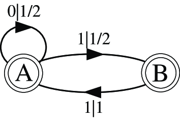
Figure 1: The even process: a strictly sofic, non-Markovian stochastic process.

We take ${L_{\mathrm{max}}}=3$ and $\alpha=0.01$. We simulated the even process for $10^{4}$ time steps and accumulated the sequence statistics for words of length $4$ and shorter, given in Table 1. Since one slides a window of size ${L_{\mathrm{max}}}+1=4$ through the data stream, there are $9,996$ length-$4$ words. Observe in Table 1 that sequences containing odd-length blocks of $1$s, bounded by $0$s, do not appear. That is, words of the form $\{01^{2k+1}0,~{}k=1,2,\ldots\}$ are forbidden.

Word	Count	Word	Count	Word	Count	Word	Count	Word	Count
0	3309	00	1654	000	836	0000	414	1000	422
1	6687	01	1655	001	818	0001	422	1001	396
		10	1655	010	0	0010	0	1010	0
		11	5032	011	1655	0011	818	1011	837
				100	818	0100	0	1100	818
				101	837	0101	0	1101	836
				110	1654	0110	814	1110	841
				111	3378	0111	841	1111	2537

Table 1: Count statistics for words of length $4$ and shorter from $10^{4}$ samples of the even process of Fig. 1. The total count at each length is $9,996$ words.

Overall, the data contains 3309 $0$s and 6687 $1$s, since for simplicity we fix the total number of words at each length to be $9,996$. The initial state $A_{L=0}$ formed at $L=0$, containing the null suffix $*\lambda$, therefore produces $1$s with probability $\approx 0.669$.

The null suffix $*\lambda$ has two children, $*0$ and $*1$. At $L=1$ the probability of producing a $1$, conditional on the suffix $*0$, is ${\rm P}(1|*0)\approx 1655/3309\approx 0.500$, which is significantly different from the distribution for the null suffix. Similarly, the probability of producing a $1$, conditional on the suffix $*1$, is ${\rm P}(1|*1)\approx 5032/6690\approx 0.752$, which is also significantly different from that of the parent state. We thus produce two new states $B_{L=1}$ and $C_{L=1}$, one containing the suffix $*1$ and one the suffix $*0$, respectively. There is now a total of three states: $A_{L=0}=\{*\lambda\}$, $B_{L=1}=\{*1\}$, and $C_{L=1}=\{*0\}$.

Examining the second generation of children at $L=2$, one finds the conditional probabilities of producing $1$s given in Table 2.

Suffix $*w$	${\rm P}(1|*w)$
*00	$818/1654\approx 0.495$
10	$837/1655\approx 0.506$
01	$1655/1655=1.000$
11	$3378/5032\approx 0.671$

Table 2: Conditional counts having read two symbols.

The morphs of the first two suffixes, $*00$ and $*10$, do not differ significantly from that of their parent $*0$, so we add them to the parent state $C_{L=1}$. But the second two suffixes, $*01$ and $*11$, must be split off from their parent $B_{L=1}$. The morph for $*01$ does not match that of $A_{L=0}$, so we create a new state $D_{L=2}=\{*01\}$. However, the morph for $*11$ does match that of $A_{L=0}$ and so we add $*11$ to $A_{L=0}$. At this point, there are four states: $A_{L=0}=\{*\lambda,*11\}$, $B_{L=1}=\{*1\}$, $C_{L=1}=\{*0,*00,*10\}$, and $D_{L=2}=\{*01\}$.

Let us examine the children of $C_{L=1}$’s $L=2$ suffixes, whose statistics are shown in Table 3.

Suffix $*w$	${\rm P}(1|*w)$
*000	$422/836\approx 0.505$
100	$396/818\approx 0.484$
010	$0/837=0.0$
110	$837/1655\approx 0.506$

Table 3: Conditional counts for child suffixes of state $C_{L=1}$’s $L=2$ suffixes.

None of these split and they are added to $C_{L=1}$.

The children of $D_{L=2}$ are given in Table 4. Again, neither of these must be split from $D_{L=2}$ and they are added to that state.

Suffix *w	${\rm P}(1|*w)$
*001	$818/818=1.000$
101	$837/837=1.000$

Table 4: Conditional counts for child suffixes of state $D_{L=2}$.

Finally, the children of $A_{L=0}$’s $L=2$ suffix are given in Table 5.

Suffix *w	${\rm P}(1|*w)$
*011	$841/1655\approx 0.508$
111	$2537/3378\approx 0.751$

Table 5: Conditional counts for child suffixes of state $A_{L=0}$’s $L=2$ suffix $*11$.

$*011$ must be split off from $A_{L=0}$, but now we must check whether its morph matches any existing distribution. In fact, its morph does not significantly differ from the morph of $C_{L=1}$, so we add $*011$ to $C_{L=1}$. $*111$ must also be split off, but its morph is similar to $B_{L=1}$’s and so it is added there. We are still left with four states, which now contain the following suffixes: $A_{L=0}=\{*\lambda,*11\}$, $B_{L=1}=\{*1,*111\}$, $C_{L=1}=\{*0,*00,*10,*000,*100,*110,*011\}$, and $D_{L=2}=\{*01,*001,*101\}$.

Since we have come to the longest histories, ${L_{\mathrm{max}}}=3$, with which we are working, Procedure II (Homogenize) is complete. We begin Procedure III by checking which states have incoming transitions. (We now drop the time-of-creation subscript.) State $C$ can be reached either from itself, state $A$, or state $B$, all on a $0$. State $C$ is reached from $D$ on a $1$ and state $D$ can be reached from state $C$ on a $1$. Finally, state $A$ can only be reached from $B$ on a $1$ and $B$ only on a $1$ from $A$. Figure 2 shows the resulting estimated full $\epsilon$-machine, with transition probabilities.

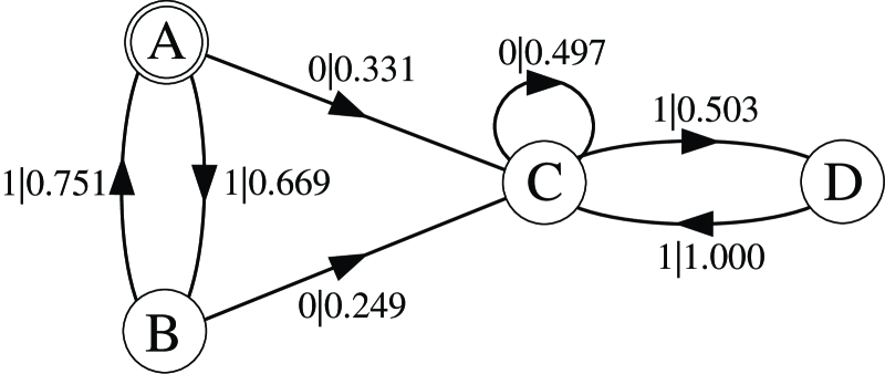
Figure 2: The full $\epsilon$-machine reconstructed from $10^{4}$ samples of the even process of Fig. 1. State $A$ (inscribed circle) is the unique start state.

Continuing on, though, we note that states $A$ and $B$ are transient. Accordingly, we eliminate them and go on to check for determinism. Every suffix in state $C$ goes to one in state $C$ by adding a $0$ and to one in state $D$ by adding a $1$, so we do not split $C$. Similarly, every suffix in $D$ goes to one in $C$ on adding a $1$, and state $D$ never produces $0$s. Hence $D$ also does not need to be changed. Since both states are future-resolving, the system of states is too, and we exit the determinization loop. Finally, we have not created any new states while determinizing, so we do not need to prune new transient states.

The final result is an $\epsilon$-machine with the two states $C$ and $D$ and with the estimated labeled transition probabilities

$${\widehat{\rm T}}^{(0)}=\left[\begin{matrix}0.497&0\cr 0&0\cr\end{matrix}\right] ~{}{\rm and}~{} {\widehat{\rm T}}^{(1)}=\left[\begin{matrix}0&0.503\cr 1.000&0\cr\end{matrix}\right]~{}.$$

We have just seen CSSR reconstruct the even process with length-$3$ histories. Nonetheless, it is important to realize that the even process is not a third-order Markov chain. Since it matters whether the current block of $1$s is of even or odd length, the process has a kind of infinite memory. It is in fact strictly sofic (Weiss, 1973), meaning that, while it has a finite number of states, it is not equivalent to a Markov chain of any finite order. For this reason conventional Markov-model techniques find it difficult to learn strictly sofic processes. In fact, many standard methods cannot handle them at all. CSSR’s ability to do so follows quite naturally from its design, dictated in turn by the basic results of computational mechanics. (For more on these points, see Section 5.1.)

3.3 Time Complexity

Procedure I (Initialize) must compute the relative frequency of all words in the data stream, up to length ${L_{\mathrm{max}}}+1$. We can accomplish this in a single pass through the data, storing the frequencies in a parse tree, with total time proportional to the number $N$ of symbols in the data stream. Thereafter we never need to refer to the data again, just the parse tree.

Procedure II (Homogenize) checks, for each suffix, whether it belongs to the same state as its parent. This operation, along with repartitioning and the creation of a new state, if needed, can all be done in constant time (through use of a hash table). Since there are at most $s(k,{L_{\mathrm{max}}})=(k^{{L_{\mathrm{max}}}+1}-1)/(k-1)$ suffixes, the total time for Procedure II is proportional to $s(k,{L_{\mathrm{max}}})$. Asymptotically, this is $O(k^{L_{\mathrm{max}}})$.

We can divide the time needed for Procedure III (Determinize) into three parts: getting the transition structure, removing transient states, and determinizing. (We remove transient states twice, but this only introduces a constant factor.) The time to find the transition structure is at most $ks(k,{L_{\mathrm{max}}})$. Removing transients can be done by finding the strongly connected components of the state-transition graph, and then finding the recurrent part of the component graph; both operations take a time proportional to the number of nodes and edges in the state-transition graph. The number of nodes can’t be more than $s(k,{L_{\mathrm{max}}})$, since there must be at least one suffix in each. Similarly the number of edges can’t be more than $ks(k,{L_{\mathrm{max}}})$ — i.e., $k$ edges per suffix. Hence transient-removal is $O(s(k,{L_{\mathrm{max}}})(k+1))=O(k^{{L_{\mathrm{max}}}+1}+k^{L_{\mathrm{max}}})=O(k^{{L_{\mathrm{max}}}+1})$. The time needed to make one determinizing pass is $ks(k,{L_{\mathrm{max}}})$, and the maximum number of passes needed is $s(k,{L_{\mathrm{max}}})$, since this is the worst case for the number of states which could be made. So the worst-case time for determinization is $O(ks^{2}(k,{L_{\mathrm{max}}}))=O(k^{2{L_{\mathrm{max}}}+1})$. Adding up for Procedure III, we get $O(k^{{L_{\mathrm{max}}}+1}+k^{{L_{\mathrm{max}}}+1}+k^{2{L_{\mathrm{max}}}+1})=O(k^{2{L_{\mathrm{max}}}+1})$. Note that if removing transients consumes the maximal amount of time, then determinization cannot and vice versa.

Putting this together, we get $O(k^{L_{\mathrm{max}}})+O(k^{2{L_{\mathrm{max}}}+1})+O(N)$, which is ${O(k^{2{L_{\mathrm{max}}}+1})+O(N)}$ asymptotically. Observe that this is linear in the data size $N$. It is exponential in the alphabet size $k$, but the exponent of $2{L_{\mathrm{max}}}+1$ is very much a loose worst-case result. It applies only in extreme cases; e.g., when every string spawns its own state, almost all of which are transient. In practice, the run time is much shorter than this bound would lead one to fear. Average-case results would replace the number of strings, here bounded by $s(k,{L_{\mathrm{max}}})\approx k^{L_{\mathrm{max}}}$, with the typical number of distinct sequences of length ${L_{\mathrm{max}}}$ the process generates with positive probability, which is $2^{{L_{\mathrm{max}}}{h_{\mu}}}$ (Cover and Thomas, 1991). Similarly, bounding the number of states by $s(k,{L_{\mathrm{max}}})$ is generally excessive.

4 Reliability and Rates of Convergence

We wish to show that the estimated $\epsilon$-machines produced by the CSSR algorithm converge to the original process’s true $\epsilon$-machine. Specifically, we will show that the set $\boldsymbol{\widehat{\mathcal{S}}}$ of states it estimates converges in probability to the correct set $\boldsymbol{{\cal S}}$ of causal states: i.e., the probability that $\boldsymbol{\widehat{\mathcal{S}}}\neq\boldsymbol{{\cal S}}$ goes to zero as $N\rightarrow\infty$. To do this, we first look at the convergence of the empirical conditional frequencies to the true morphs and then use this to show that the set $\boldsymbol{\widehat{\mathcal{S}}}$ of states converges. Finally, we examine the convergence of predictions once the causal states are established and say a few words about how, from a dynamical-systems viewpoint, the $\epsilon$-machine acts as a kind of attractor for the algorithm.

Throughout, we make the following assumptions:

1. The process is conditionally stationary. Hence the ergodic theorem for stationary processes applies (Grimmett and Stirzaker, 1992, Sec. 9.5) and time averages converge almost surely to the state-space average for whatever ergodic component the process happens to be in.

2. The original process has only a finite number of causal states.

3. Every state contains at least one suffix of finite length. That is, there is some finite $L$ such that every state contains a suffix of length no more than $L$. This does not mean that $L$ symbols of history always suffice to determine the state, just that it is possible to synchronize — in the sense of Upper (1997) — to every state after seeing no more than $L$ symbols.

We also assume that CSSR estimates conditional probabilities (morphs) by simple maximum likelihood. One can substitute other estimators — e.g., maximum entropy — and only the details of the convergence arguments would change.

4.1 Convergence of the Empirical Conditional Probabilities to the Morphs

The past $\stackrel{{\scriptstyle\leftarrow}}{{S}}$ and the future $\stackrel{{\scriptstyle\rightarrow}}{{S}}$ of the process are independent given the causal state $\sigma\in{\cal S}$ (Prop. 3). More particularly, the past $\stackrel{{\scriptstyle\leftarrow}}{{S}}$ and the next future symbol ${\stackrel{{\scriptstyle\rightarrow}}{{S}}}^{1}$ are independent given the causal state. Hence, $\stackrel{{\scriptstyle\leftarrow}}{{S}}$ and ${\stackrel{{\scriptstyle\rightarrow}}{{S}}}^{1}$ are independent, given a history suffix sufficient to fix us in a cell of the causal-state partition. Now, the morph for that suffix is a multinomial distribution over $\cal A$, which gets sampled independently each time the suffix occurs. Our estimate of the morph is the empirical distribution obtained by IID samples from that multinomial. Write this estimated distribution as $\widehat{{\rm P}}_{N}({\stackrel{{\scriptstyle\rightarrow}}{{S}}}^{1}=a|{\stackrel{{\scriptstyle\leftarrow}}{{S}}}^{L}={\stackrel{{\scriptstyle\leftarrow}}{{s}}}^{L})$, recalling that ${\rm P}({\stackrel{{\scriptstyle\rightarrow}}{{S}}}^{1}=a|{\stackrel{{\scriptstyle\leftarrow}}{{S}}}^{L}={\stackrel{{\scriptstyle\leftarrow}}{{s}}}^{L})$ denotes the true morph. Does $\widehat{{\rm P}}_{N}\rightarrow{\rm P}$ as $N$ grows?

Since we use the KS test, it is reasonable to employ the variational distance. Given two distributions $P$ and $Q$ over $\mathcal{A}$, the variational distance is

$$d(P,Q)=\sum_{a\in\mathcal{A}}{|P(X=a)-Q(X=a)|}~{}.$$ (9)

Scheffé showed that

$$d(P,Q)=2\max_{\mathrm{A}\in 2^{\mathcal{A}}}{|P(X\in\mathrm{A})-Q(X\in\mathrm{A})|}~{},$$ (10)

where $2^{\mathcal{A}}$ is the power-set of $\mathcal{A}$, of cardinality $2^{k}$ (Devroye and Lugosi, 2001).

Chernoff’s inequality (Vidyasagar, 1997) tells us that, if $X_{1},X_{2},\ldots X_{n}$ are IID Bernoulli random variables and $A_{n}$ is the mean of the first $n$ of the $X_{i}$, with probability $\mu$ of success, then

$${{\rm P}(|A_{n}-\mu|\geq t)}\leq 2e^{-2nt^{2}}~{}.$$ (11)

Applying this to our estimation problem and letting $n=\nu({\stackrel{{\scriptstyle\leftarrow}}{{s}}}^{L})$ be the number of times we have seen the suffix ${\stackrel{{\scriptstyle\leftarrow}}{{s}}}^{L}$, we have:

$${\rm P}(d(\widehat{{\rm P}}_{n}({\stackrel{{\scriptstyle\rightarrow}}{{S}}}^{1}|{\stackrel{{\scriptstyle\leftarrow}}{{S}}}^{L}={\stackrel{{\scriptstyle\leftarrow}}{{s}}}^{L}),{\rm P}({\stackrel{{\scriptstyle\rightarrow}}{{S}}}^{1}|{\stackrel{{\scriptstyle\leftarrow}}{{S}}}^{L}={\stackrel{{\scriptstyle\leftarrow}}{{s}}}^{L}))\geq t)$$ (12)

$$= {\rm P}\left(t<\sum_{a\in\mathcal{A}}{\left|\widehat{{\rm P}}_{n}({\stackrel{{\scriptstyle\rightarrow}}{{S}}}^{1}=a|{\stackrel{{\scriptstyle\leftarrow}}{{S}}}^{L}={\stackrel{{\scriptstyle\leftarrow}}{{s}}}^{L})-{\rm P}({\stackrel{{\scriptstyle\rightarrow}}{{S}}}^{1}=a|{\stackrel{{\scriptstyle\leftarrow}}{{S}}}^{L}={\stackrel{{\scriptstyle\leftarrow}}{{s}}}^{L})\right|}\right)$$ (13)

$$= {\rm P}\left(2t<\max_{\mathrm{A}\in 2^{\mathcal{A}}}{\left|\widehat{{\rm P}}_{n}({\stackrel{{\scriptstyle\rightarrow}}{{S}}}^{1}\in\mathrm{A}|{\stackrel{{\scriptstyle\leftarrow}}{{S}}}^{L}={\stackrel{{\scriptstyle\leftarrow}}{{s}}}^{L})-{\rm P}({\stackrel{{\scriptstyle\rightarrow}}{{S}}}^{1}\in\mathrm{A}|{\stackrel{{\scriptstyle\leftarrow}}{{S}}}^{L}={\stackrel{{\scriptstyle\leftarrow}}{{s}}}^{L})\right|}\right)$$ (14)

$$\leq \sum_{\mathrm{A}\in 2^{\mathcal{A}}}{{\rm P}\left(\left|\widehat{{\rm P}}_{n}({\stackrel{{\scriptstyle\rightarrow}}{{S}}}^{1}\in\mathrm{A}|{\stackrel{{\scriptstyle\leftarrow}}{{S}}}^{L}={\stackrel{{\scriptstyle\leftarrow}}{{s}}}^{L})-{\rm P}({\stackrel{{\scriptstyle\rightarrow}}{{S}}}^{1}\in\mathrm{A}|{\stackrel{{\scriptstyle\leftarrow}}{{S}}}^{L}={\stackrel{{\scriptstyle\leftarrow}}{{s}}}^{L})\right|>2t\right)}$$ (15)

$$\leq \sum_{\mathrm{A}\in 2^{\mathcal{A}}}{2{e}^{-2n{(2t)}^{2}}}$$ (16)

$$= 2^{k+1}{e}^{-8n{t}^{2}}~{}.$$ (17)

Thus, the empirical conditional distribution (morph) for each suffix converges exponentially fast to its true value, as the suffix count $n$ grows.

Suppose there are $s$ suffixes across all the states. We have seen the $i^{\rm th}$ suffix $n_{i}$ times; abbreviate the $s$-tuple $(n_{1},\ldots n_{s})$ by $\mathbf{n}$. We want the empirical distribution associated with each suffix to be close to the empirical distribution of all the other suffixes in its state. We can ensure this by making all the empirical distributions close to the state’s morph. In particular, if all distributions are within $t$ of the morph, then (by the triangle inequality) every distribution is within $2t$ of every other distribution. Call the probability that this is not true $q(t,\mathbf{n})$. This is the probability that at least one of the empirical distributions is not within $t$ of the state’s true morph. $q(t,\mathbf{n})$ is at most the sum of the probabilities of each suffix being an outlier. Hence, if there are $s$ suffixes in total, across all the states, then the probability that one or more suffixes differs from its true morph by $t$ or more is

$$q(t,\mathbf{n}) \leq \sum_{i=1}^{s}{2k{e}^{-8n_{i}t^{2}}}$$ (18)

$$\leq 2^{k+1}s{e}^{-8mt^{2}}~{},$$ (19)

where $m$ is the least of the $n_{i}$. Now, this formula is valid whether we interpret $s$ as the number of histories actually seen or as the number of histories needed to infer the true states. In the first case, Eq. (19) tells us how accurate we are on the histories seen; in the latter, over all the ones we need to see. This last is clearly what we need to prove overall convergence, but knowing $s$, in that sense, implies more knowledge of the process’s structure than we start with. However, we can upper bound $s$ by the maximum number of morphs possible — $s\leq(k^{L+1}-1)/(k-1)$ — so we only need to know (or, in practice, pick) $L$.

Which string is least-often seen — which $n_{i}$ is $m$ — generally changes as more data accumulates. However, we know that the frequencies of strings converge almost surely to probabilities as $N\rightarrow\infty$. Since there are only a finite number of strings of length $L$ or less, it follows that the empirical frequencies of all strings also converge almost surely. If $p^{*}$ is the probability of the most improbable string, then $m\rightarrow Np^{*}$ almost surely. Hence, for sufficiently large $N$,

$$q(t,\mathbf{n}) \leq 2^{k+1}\frac{k^{L}-1}{k-1}e^{-8Np^{*}t^{2}}~{},$$ (20)

which vanishes with $N$.

We can go further by invoking the assumption that there are only a finite number of causal states. This means that causal states form a finite irreducible Markov chain. The empirical distributions over finite sequences generated by such chains converge exponentially fast to the true distribution (den Hollander, 2000). (The rate of convergence depends on the entropy ${\cal D}(\widehat{{\rm P}}|{\rm P})$ of the empirical distribution relative to the true.) Our observed process is a random function of the process’s causal states. Now, for any pair of distributions $P(X)$ and $Q(X)$ and any measurable function $f:X\rightarrow Y$,

$$d(P(X),Q(X))\geq d(P(Y),Q(Y))~{},$$ (21)

whether $f$ is either a deterministic or a random function. Hence, the empirical sequence distribution, at any finite length, converges to the true distribution at least as quickly as the state distributions. That is, they converge with at least as large an exponent. Therefore, under our assumptions, for each $i$, $n_{i}/N\rightarrow p_{i}$ exponentially fast — there is an increasing function $r(\varepsilon)$, $r(0)=0$, and a constant $C$ such that, for each $\varepsilon\geq 0$,

$${\rm P}\left(\left|\frac{n_{i}}{N}-p_{i}\right|>\varepsilon\right) \leq Ce^{-Nr(\varepsilon)}~{}.$$ (22)

($r(\varepsilon)$ is known as the large-deviation rate function.) The probability that $m\leq N(p^{*}-\varepsilon)$ is clearly no more than the probability that, for one or more $i$, $n_{i}\leq N(p^{*}-\varepsilon)$. Since the lowest-probability strings need to make the smallest deviations from their expectations to cause this, the probability that at least one $n_{i}$ is below $N(p^{*}-\varepsilon)$ is no more than $k^{L}$ times the probability that the count of the least probable string is below $N(p^{*}-\varepsilon)$. The probability that an empirical count $n_{i}$ is below its expectation by $\varepsilon$, in turn, is less than the probability that it deviates from its expectation by $\varepsilon$ in either direction. That is,

$${\rm P}(m\leq N(p^{*}-\varepsilon)) \leq {\rm P}\left(\bigcup_{i}{n_{i}\leq N(p^{*}-\varepsilon)}\right)$$ (23)

$$\leq \sum_{i}{{\rm P}(n_{i}\leq N(p^{*}-\varepsilon))}$$ (24)

$$\leq k^{L}{\rm P}(n^{*}\leq{N}(p^{*}-\varepsilon))$$ (25)

$$\leq k^{L}{\rm P}\left(\left|\frac{n^{*}}{N}-p^{*}\right|>\varepsilon\right)$$ (26)

$$\leq Ck^{L}e^{-Nr(\varepsilon)}~{}.$$ (27)

With a bound on $m$, we can fix an overall exponential bound on the error probability $q$:

$$q(t,\mathbf{n})\leq\inf_{\varepsilon\geq 0}{C2^{k+1}k^{L}\frac{k^{L+1}-1}{k-1}e^{-8N(p^{*}-\varepsilon)t^{2}}e^{-Nr(\varepsilon)}}~{}.$$ (28)

Solving out the infimum would require knowledge of $r(\epsilon)$, which is difficult to come by. Whatever $r(\epsilon)$ may be, however, the bound is still exponential in $N$.

The above bound is crude for small $N$ and especially for small $t$. In the limit $t\rightarrow 0$, it tells us that a probability is less than some positive integer, which, while true, is not at all sharp. It becomes less crude, however, as $N$ and $t$ grow. In any case, it suffices for the present purposes.

We can estimate $p^{*}$ from the reconstructed $\epsilon$-machine by calculating its fluctuation spectrum (Young and Crutchfield, 1993). Young and Crutchfield demonstrated that the estimates of $p^{*}$ obtained in this way become quite accurate with remarkably little data, just as estimates of the entropy rate ${h_{\mu}}$ do. At the least, calculating $p^{*}$ provides a self-consistency check on the reconstructed $\epsilon$-machine.

4.2 Analysis of Error Probabilities

Let us consider the kinds of statistical error each of the algorithm’s three procedures can produce.

Since it merely sets up parameters and data structures, nothing goes wrong in Procedure I (Initialize).

Procedure II (Homogenize) can make two kinds of errors. First, it can group together histories with different distributions for the next symbol. Second, it can fail to group together histories that have the same distribution. We will analyze both cases together.

It is convenient here to introduce an additional term. By analogy with the causal states, the precausal states are defined by the following equivalence relation: Two histories are precausally equivalent when they have the same morph. The precausal states are then the coarsest states (partition) that are weakly prescient. The causal states are either the same as the precausal states or a refinement of them. Procedure II ought to deliver the correct partition of histories into precausal states.

Suppose ${\stackrel{{\scriptstyle\leftarrow}}{{s}}}_{i}$ and ${\stackrel{{\scriptstyle\leftarrow}}{{s}}}_{j}$ are suffixes in the same state, with counts $n_{i}$ and $n_{j}$. No matter how large their counts, there is always some variational distance $t$ such that the significance test will not separate estimated distributions differing by $t$ or less. If we make $n_{i}$ large enough, then, with probability arbitrarily close to one, the estimated distribution for ${\stackrel{{\scriptstyle\leftarrow}}{{s}}}_{i}$ is within $t/2$ of the true morph, and similarly for ${\stackrel{{\scriptstyle\leftarrow}}{{s}}}_{j}$. Thus, the estimated morphs for the two suffixes are within $t$ of each other and will be merged. Indeed, if a state contains any finite number of suffixes, by obtaining a sufficiently large sample of each, we can ensure (with arbitrarily high probability) that they are all within $t/2$ of the true morph and so within $t$ of each other and thus merged. In this way, the probability of inappropriate splitting can be made arbitrarily small.

If each suffix’s conditional distribution is sufficiently close to its true morph, then any well behaved test will eventually separate suffixes that belong to different morphs. More concretely, let the variational distance between the morphs for the pair of states $\sigma_{i}$ and $\sigma_{j}$ be $d_{ij}$. A well behaved test will distinguish two samples whose distance is some constant fraction of this or more — say, $3d_{ij}/4$ or more — if $n_{i}$ and $n_{j}$ are large enough. By taking $n_{i}$ large enough, we can make sure, with probability arbitrarily close to $1$, that the estimated distribution for $\sigma_{i}$ is within some small distance of its true value — say, $d_{ij}/8$. We can do the same for $\sigma_{j}$ by taking $n_{j}$ large enough. Therefore, with probability arbitrarily close to one, the distance between the estimated morphs for $\sigma_{i}$ and $\sigma_{j}$ is at least $3d_{ij}/4$, and $i$ and $j$ are, appropriately, separated. Hence, the probability of erroneous non-separations can be made as small as desired.

Therefore, by taking $N$ large enough, we can make the probability that the correct precausal states are inferred arbitrarily close to $1$.

If every history is correctly assigned to a precausal state, then nothing can go wrong in Procedure III (Determinize). Take any pair of histories ${\stackrel{{\scriptstyle\leftarrow}}{{s}}}_{1}$ and ${\stackrel{{\scriptstyle\leftarrow}}{{s}}}_{2}$ in the same precausal state: either they belong to the same causal state or they do not. If they do belong to the same causal state, then by determinism, for every string $w$, ${\stackrel{{\scriptstyle\leftarrow}}{{s}}}_{1}w$ and ${\stackrel{{\scriptstyle\leftarrow}}{{s}}}_{2}w$ belong to the same causal state. Since the causal states are refinements of the precausal states, this means that ${\stackrel{{\scriptstyle\leftarrow}}{{s}}}_{1}w$ and ${\stackrel{{\scriptstyle\leftarrow}}{{s}}}_{2}w$ also belong to the same precausal state. Contrarily, if ${\stackrel{{\scriptstyle\leftarrow}}{{s}}}_{1}$ and ${\stackrel{{\scriptstyle\leftarrow}}{{s}}}_{2}$ belong to different causal states, they must give different probabilities for some strings. Pick the shortest such string $w$ (or any one of them, if there is more than one) and write it as $w=va$, where $a$ is a single symbol. Then the probability of $a$ depends on whether we saw ${\stackrel{{\scriptstyle\leftarrow}}{{s}}}_{1}v$ or ${\stackrel{{\scriptstyle\leftarrow}}{{s}}}_{2}v$. So ${\stackrel{{\scriptstyle\leftarrow}}{{s}}}_{1}v$ and ${\stackrel{{\scriptstyle\leftarrow}}{{s}}}_{2}v$ have distinct morphs and belong to different precausal states. Hence, determinization will separate ${\stackrel{{\scriptstyle\leftarrow}}{{s}}}_{1}$ and ${\stackrel{{\scriptstyle\leftarrow}}{{s}}}_{2}$, since, by hypothesis, the precausal states are correct. Thus, histories will always be separated, if they should be, and never, if they should not.

Since determinization always refines the partition with which it starts and the causal states are a refinement of the precausal states, there is no chance of merging histories that do not belong together. Hence, Procedure III will always deliver the causal states, if it starts with the precausal states. We will not examine the question of whether Procedure III can rectify a mistake made in Procedure II. Experientially, this depends on the precise way determinization is carried out and, most typically, if the estimate of the precausal states is seriously wrong, determinization only compounds the mistakes. Procedure III does not, however, enhance the probability of error.

To conclude: If the number of causal states is finite and ${L_{\mathrm{max}}}$ is sufficiently large, the probability that the states estimated are not the causal states becomes arbitrarily small, for sufficiently large $N$. Hence the CSSR algorithm, considered as an estimator, is (i) consistent (Cramér, 1945), (ii) probably approximately correct (Kearns and Vazirani, 1994, Vapnik, 2000), and (iii) reliable (Spirtes et al., 2001, Kelly, 1996), depending on which field one comes from.

4.3 Dynamics of the Learning Algorithm

Figure 3: Number of states inferred as a function of history length ${L_{\mathrm{max}}}$ and data size $N$ for the even process of Section 3.2. The true number of states is 2. Curves are averages over 30 independent realizations at each $N$. Here, and in subsequent figures, the significance level $\alpha$ was fixed to ${10}^{-3}$.

We may consider the CSSR algorithm itself to be a stochastic dynamical system, moving through a state space of possible history-partitions or $\epsilon$-machines. What we have seen is that the probability that CSSR does not infer the correct states (partition) — that it does not have the causal architecture right — drops exponentially as time goes on. By the Borel-Cantelli lemma, therefore, CSSR outputs $\epsilon$-machines that have the wrong architecture only finitely many times before fixing on the correct architecture forever. Thus, the proper architecture is a kind of absorbing region in $\epsilon$-machine space. In fact, almost all of the algorithm’s trajectories end up there and stay. (There may be other absorbing regions, but only a measure-$0$ set of inference trajectories reach them.)

Because CSSR can only create new states as it steps through $L$ to ${L_{\mathrm{max}}}$, it is tempting to conjecture that CSSR “converges from below” — that the number of states grows monotonically from one to the true value, perhaps for growing $N$ with fixed ${L_{\mathrm{max}}}$, or for growing ${L_{\mathrm{max}}}$ with fixed $N$. This is not so, however. If ${L_{\mathrm{max}}}$ is too large relative to $N$ (see Section 4.4), the probabilities of long strings will not be consistently estimated, so the hypothesis tests in Procedure II become unreliable and tend to produce too many states. Procedure III then amplifies this excess. More broadly, after Procedure II makes the precausal states, Procedure III determinizes them, and the deterministic version of an incorrect set of states (e.g., from setting ${L_{\mathrm{max}}}$ too small) can easily be larger than the correct $\epsilon$-machine. The general situation, illustrated by Figure 3, does not allow us to make any generalization about convergence “from above” or “from below”.

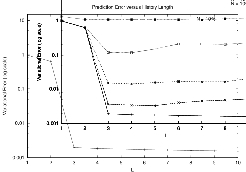
Figure 4: Prediction error (logarithmic scale) as a function of history length and data size. The figure depicts the total-variation distance between the actual distribution over words of length 10, and that implied by the inferred model (true generalization error). Error is shown as a function of ${L_{\mathrm{max}}}$ (running from 1 to 10) and $N$ (running from ${10}^{2}$ to ${10}^{6}$), averaged over 30 independent realizations at each $N$.

Figure 5: Scaling of prediction error (linear scale) as a function of $N$. As in Figure 4, but the variational distance is now scaled by a factor of $\sqrt{N}$. For clarity, we have restricted ${L_{\mathrm{max}}}$ to the range 3–10, since 3 is the smallest value of ${L_{\mathrm{max}}}$ for which CSSR can find the correct model. At this significance level, CSSR never finds the correct model for $N={10}^{2}$, and only sporadically for $N={10}^{3}$, hence those lines do not fall on the scaling curve.

We are not satisfied with getting the correct causal architecture, however. We also want the morphs to converge. Here we can exploit the fact that the estimated morph for each causal state is an average over the histories it contains. If there are $s_{c}$ causal states and the least frequently sampled one has been seen $m_{c}$ times, then reasoning parallel to that in Section 4.1 above tells us that the probability any of our estimated morphs differs from its true morph by $t$ or more is at most $2^{k+1}s_{c}exp(-8m_{c}t^{2})$. Moreover, since the causal states form an irreducible Markov chain, $m_{c}$ will converge exponentially quickly to $Np^{*}_{c}$.

As a general note, while the probability of errors of a given size goes down exponentially with $N$, this does not imply that the expectation of the error is exponentially decreasing. Rather, the expected variational difference between the true and empirical distributions for a multinomial goes as $N^{-1/2}$ (Devroye and Lugosi, 2001). Since $N$ appears in the form for the error probability only in the combination $Np^{*}_{c}$, we expect a variational error scaling as $1/\sqrt{Np^{*}_{c}}$. Readers may judge the quality of the data-collapse of the rescaled error for themselves from Figures 4 and 5.

4.4 Choice of Algorithm Parameters

CSSR has two adjustable parameters: the maximum history length used, ${L_{\mathrm{max}}}$, and the significance level $\alpha$.

We have seen that there is a lower bound for the acceptable value of ${L_{\mathrm{max}}}$, namely, it must be large enough that every state contains at least one suffix of that length. Let us call this least acceptable value $\Lambda$. If ${L_{\mathrm{max}}}<\Lambda$, our proof of convergence fails, and in general neither CSSR nor any other procedure can reconstruct the causal states using histories of length ${L_{\mathrm{max}}}$. For periodic processes, for instance, $\Lambda$ is equal to the period. Since the statistical complexity ${C_{\mu}}$ of a process with period $p$ is just $\log{p}$, this suggests that generally $\Lambda\approx 2^{C_{\mu}}$, but this is unproven, and we know of no estimator for ${C_{\mu}}$ other than direct reconstruction.

Rather than try to determine $\Lambda$, one might use the largest ${L_{\mathrm{max}}}$ compatible with available memory (and one’s own impatience). However, the size of the data-set $N$ limits the permissible values of ${L_{\mathrm{max}}}$. We can see this as follows. Estimating the distribution for the next symbol conditional on a history of length $L-1$ is equivalent to estimating the distribution of strings of length $L$. Now, the asymptotic equipartition property (Cover and Thomas, 1991) tells us that the number of strings which appear with positive probability grows as $2^{L{h_{\mu}}}$. That is, the number of probabilities we need to estimate grows exponentially with $L$. To get an adequate number of samples per string thus requires an exponentially growing amount of data. Conversely, adequate sampling limits $L$ to be, at most, on the order of the logarithm of $N$.

A result of Marton and Shields (1994) makes this more precise. Let $L(N)$ be the the maximum $L$ we can use when we have $N$ data-points. If the observed process satisfies the weak Bernoulli property (which random functions of irreducible Markov chains do), then a sufficient condition for the convergence of sequence probability estimates is that $L(N)\leq\log{N}/({h_{\mu}}+\varepsilon)$, for some positive $\varepsilon$. One might wonder if cleverness could improve this; but Marton and Shields also showed that, if $L(N)\geq\log{N}/{h_{\mu}}$, probability estimates over length $L$ words do not converge. We must know ${h_{\mu}}$ to use this result, but $\log{k}\geq{h_{\mu}}$, so we can err on the side of caution by substituting the log of the alphabet size for the entropy rate. For a given process and data-set, it is of course possible that $L(N)<\Lambda$, in which case we simply haven’t enough data to reconstruct the true model.

As to the significance level $\alpha$, the proof of convergence shows us that it doesn’t matter, at least asymptotically in $N$: histories with distinct morphs will be put in separate states, and histories with the same morph will be joined together in the same state. In the meanwhile, with finite data, it does affect the kind of error CSSR makes. The significance level is the probability that two samples, drawn from the same distribution, would be split apart by the test. If $\alpha$ is small, therefore, we will split only on large values of the test statistic — only (as it were) glaringly obvious distinctions between empirical distributions will lead to splits. To become sensitive to very small distinctions between states, we need either large quantities of data, or a high significance level, which would make us more likely to split accidentally. The significance level therefore indicates our willingness to risk seeing structure that isn’t really there, i.e., creating states due merely to sampling error.

5 Comparison with Earlier Techniques

In this section, we compare CSSR to two classes of existing techniques for pattern discovery in time series: “context” or variable-length Markov models, and state-merging methods for causal state reconstruction. We see that the “context” methods are actually included as a special case of causal state reconstruction, under restrictive, and generally under-appreciated, assumptions. Merging methods for state reconstruction, while they have the same domain of applicability as CSSR, are less well-behaved, and converge more slowly.

5.1 Variable-Length Markov Models

The “context” algorithm of Rissanen (1983) and its descendants (Bühlmann and Wyner, 1999, Willems et al., 1995, Tino and Dorffner, 2001) construct so-called “variable-length Markov models” (VLMMs) from sequence data. The object is to find a set of contexts such that, given the context, the past of the sequence and its next symbol are conditionally independent. Contexts are taken to be suffixes of the history, and the algorithms work by examining increasingly long histories, creating new contexts by splitting existing ones into longer suffixes when thresholds of error are exceeded. (This means that contexts can be arranged in a tree, so these are also called “context tree” or “probabilistic suffix tree” algorithms.)

This description of variable-length Markov model algorithms makes it clear that they are related to causal state reconstruction, and, like reconstruction algorithms, they infer both architecture and parameters. However, causal state methods have several important advantages over VLMM methods. First, we use the known properties of the states we are looking for to guide search. Second, rather than creating states when we cross some arbitrary threshold for, say, the Kullback-Leibler divergence, we use well-understood statistical tests for identity of distribution. Third, context methods suffer from the following defect. Each state they infer is represented by a single suffix. That is, their states consist of all and only the histories ending in a particular suffix. For many processes, the causal states contain multiple suffixes. In these cases, multiple “contexts” are needed to represent a single causal state, so VLMMs are generally more complicated than $\epsilon$-machines.

Recall the even process of Section 3.2. It has two recurrent causal states, labeled A and B in Figure 1. Any history terminated by a 0, or by a 0 followed by an even number of 1s, belongs to state A. Any history terminated by a 0 followed by an odd number of 1s, belongs to B. Clearly A and B both contain infinitely many suffixes, and so correspond to an infinite number of contexts. VLMM algorithms are simply incapable of capturing this structure. If we let ${L_{\mathrm{max}}}$ grow, a VLMM algorithm will increase the number of contexts it finds without bound, but cannot achieve the same combination of predictive power and model simplicity as causal state reconstruction.

Moreover, the even process is not an isolated pathological case. Rather, it is a prototype of the strictly sofic processes (Weiss, 1973, Badii and Politi, 1997), which are, in essence, processes which can be described as hidden Markov models, but are not Markov chains of any finite order. VLMMs cannot capture strictly sofic processes, for the same reason they cannot capture the even process. However, sofic processes are simply regular languages, since they have only finitely many states. Causal states cannot provide a finite representation of every regular language (Upper, 1997, Crutchfield, 1994), but the class they capture strictly includes those captured by VLMMs.

5.2 State-Merging $\epsilon$-Machine Inference Algorithms

Existing $\epsilon$-machine reconstruction procedures use what one might call state compression or merging. The default assumption is that each distinct history encountered in the data is a distinct causal state. Histories are then merged into causal states when their morphs are close. Kindred merging procedures can learn hidden Markov models (Stolcke and Omohundro, 1993) and finite automata (Trakhtenbrot and Barzdin, 1973, Murphy, 1996).

The standard $\epsilon$-machine inference algorithm is the subtree-merging algorithm introduced by Crutchfield and Young (Crutchfield and Young, 1989, 1990). The algorithm begins by building a $k$-ary tree of some pre-set depth $D$, where paths through the tree correspond to sequences of observations of length $D$, obtained by sliding a length-$D$ window through the data stream (or streams, if there are several). If $D=4$, say, and the sequence $abba$ is encountered, the path in the tree will start at the root node, take the edge labeled $a$ to a new node, then take the outgoing edge labeled $b$ to a third node, then the edge labeled $b$ from that, and finally the edge labeled $a$ to a fifth node, which is a leaf. An edge of the tree is labeled, not just with a symbol, but also with the number of times that edge has been traversed in scanning through the data stream. Denote by $\nu(a_{i}|n)$ the number on the $a_{i}$ edge going out of node $n$ and $N$ the total number of sequences entered into the tree. The tree is a $D$-block Markov model of the process. Each level $l$ gives an estimate of the distribution of length-$l$ words in the data stream.

The traversal-counts are converted into empirical conditional probabilities by normalization:

$${\widehat{{\rm P}}_{N}}(a_{i}|n) = \frac{\nu(a_{i}|n)}{\sum_{a_{j}}{\nu(a_{j}|n)}}~{}.$$

Thus, attached to each non-leaf node is an empirical conditional distribution for the next symbol. If node $n$ has descendants to depth $K$, then it has (by implication) a conditional distribution for futures of length $K$.

The merging procedure is now as follows. Consider all nodes with subtrees of depth $L=D/2$. Take any two of them. If all the empirical probabilities attached to the length-$L$ path in their subtrees are within some constant $\delta$ of one another, then the two nodes are equivalent. They should be merged with one another. The new node for the root will have incoming links from both the parents of the old nodes. This procedure is to be repeated until no further merging is possible. It is clear that, given enough data, a long enough $L$, and a small enough $\delta$, the subtree algorithm will converge on the causal states.

All other methods for $\epsilon$-machine reconstruction currently in use are also based on merging. Take, for instance, the “topological” or “modal” merging procedure of Perry and Binder (1999). They consider the relationship between histories and futures, both (in the implementation) of length $L$. Two histories are assigned to the same state if the sets of futures that can succeed them are identical. The distribution over those futures is then estimated for each state, not for each history.

As we said, the default assumption of current state-merging methods is that each history is its own state. The implicit null model of the process is thus the most complex possible, given the length of histories available, and is whittled down by merging. In all this, they are the opposite of CSSR. State splitting starts by putting every history in one state — a zero-complexity null model that is elaborated by splitting.

Unfortunately, state-merging has inherent difficulties. For instance: what is a reasonable value of morph similarity $\delta$? Clearly, as the amount of data increases and the law of large numbers makes empirical probabilities converge to true probabilities, $\delta$ should grow smaller. But it is grossly impractical to calculate what $\delta$ should be, since the null model itself is so complicated. (Current best practice is to pick $\delta$ as though the process were an IID multinomial, which is the opposite of the algorithm’s implicit null model.) In fact, using the same $\delta$ for every pair of tree nodes is unreliable. The nodes will not have been visited equally often, being associated with different tree depths, so the conditional probabilities in their subtrees vary in accuracy. An analysis of the convergence of empirical distributions, of the kind we made in Section 4.1 above, could give us a handle on $\delta$, but reveals another difficulty. CSSR must estimate $2^{k}$ probabilities for each history — one for each member of the power-set of the alphabet. The subtree-merging algorithm, however, must estimate the probability of each member of the power set of future sequences, i.e., $2^{k^{L}}$ probabilities. This is an exponentially larger number, and the corresponding error bounds would be worse by this factor.

The theorems in Shalizi and Crutchfield (2001) say a great deal about the causal states: they are deterministic, they are Markovian, and so on. No previous reconstruction algorithm made use of this information to guide its search. Subtree-merging algorithms can return nondeterministic states, for instance, which cannot possibly be the true causal states. While the subtree algorithm converges, and other merging algorithms probably do too, CSSR should do better, both in terms of the kind of result it delivers and the rate at which it approaches the correct result.

6 Conclusion

We briefly map out directions for future exploration, and finish by summarizing our results.

6.1 Future Directions

A number of directions for future work present themselves. Elsewhere, we have developed extensions of computational mechanics to transducers and interacting time series and to spatio-temporal dynamical systems (Hanson and Crutchfield, 1997, Shalizi, 2001, Shalizi and Crutchfield, 2002). It is clear that the present algorithm can be applied to transducers, and we feel that it can be applied to spatio-temporal systems.

One can easily extend the formalism of computational mechanics to processes that take on continuous values at discrete times, but this has never been implemented. Much of the machinery we employed here carries over straightforwardly to the continuous setting, e.g., empirical process theory for IID samples (Devroye and Lugosi, 2001) or the Kolmogorov-Smirnov test. The main obstacle to simply using CSSR in its present form is the need for continuous interpolation between the (necessarily finite) measurements. However, all methods of predicting continuous-valued processes must likewise impose some interpolation scheme. It seems likely that schemes along the lines of those used by Bosq (1998) or Fraser and Dimitriadis (1993) would work with CSSR. Continuous-valued, continuous-time processes raise more difficult questions, which we shall not even attempt to sketch here.

CSSR currently returns a single model, and so provides a “point estimate” of the causal states. This raises the question of what the corresponding confidence region would look like, and how it might be computed. Similarly, an estimate of the expected degree of over-fitting, as a function either of the number of states or of ${C_{\mu}}$, would open the way to applying the structural risk minimization principle (Vapnik, 2000).

Potentially, $\epsilon$-machines and our algorithm can be applied in any domain where HMMs have proved their value (e.g., bioinformatics (Baldi and Brunak, 1998)) or where there are poorly-understood processes generating sequential data, such as speech, in which one wishes to find non-obvious or very complex patterns.

6.2 Summary

We have presented a new algorithm for pattern discovery in time series. Given samples of a conditionally stationary process, the algorithm reliably infers the process’s causal architecture. Under certain conditions on the process, not uncommonly met in practice, the algorithm almost surely returns an incorrect architecture only finitely many times. The time complexity of the algorithm is linear in the data size. We have proved it works reliably on all processes with finitely many causal states. Finally, we have argued that CSSR will consistently outperform prior causal-state-merging algorithms and context-tree methods.

A Information Theory

Our notation and terminology follows that of Cover and Thomas (1991).

Given a random variable $X$ taking values in a discrete set $\mathcal{A}$, the entropy $H[X]$ of $X$ is

$$H[X] \equiv -\sum_{a\in\mathcal{A}}{{\rm P}(X=a)\log_{2}{{\rm P}(X=a)}}~{}.$$

$H[X]$ is the expectation value of $-\log_{2}{{\rm P}(X)}$. It represents the uncertainty in $X$, interpreted as the mean number of binary distinctions (bits) needed to identify the value of $X$. Alternately, it is the minimum number of bits needed to encode or describe $X$. Note that $H[X]=0$ if and only if $X$ is (almost surely) constant.

The joint entropy $H[X,Y]$ of two variables $X$ and $Y$ is the entropy of their joint distribution:

$$H[X,Y] \equiv -\sum_{a\in\mathcal{A},b\in\mathcal{B}}{{\rm P}(X=a,Y=b)\log_{2}{{\rm P}(X=a,Y=b)}}~{}.$$

The conditional entropy of $X$ given $Y$ is

$$H[X|Y] \equiv H[X,Y]-H[Y]~{}.$$

$H[X|Y]$ is the average uncertainty remaining in $X$, given a knowledge of $Y$.

The mutual information $I[X;Y]$ between $X$ and $Y$ is

$$I[X;Y] \equiv H[X]-H[X|Y]~{}.$$

It gives the reduction in $X$’s uncertainty due to knowledge of $Y$ and is symmetric in $X$ and $Y$.

The entropy rate ${h_{\mu}}$ of a stochastic process $\ldots,S_{-2},S_{-1},S_{0},S_{1},S_{2},\ldots$ is

$${h_{\mu}} \equiv \lim_{{L\rightarrow\infty}}{H[{\stackrel{{\scriptstyle\rightarrow}}{{S}}}^{1}|{\stackrel{{\scriptstyle\leftarrow}}{{S}}}^{L}]}$$

$$= H[{\stackrel{{\scriptstyle\rightarrow}}{{S}}}^{1}|\stackrel{{\scriptstyle\leftarrow}}{{S}}]~{}.$$

(The limit always exists for conditionally stationary processes.) ${h_{\mu}}$ measures the process’s unpredictability, in the sense that it is the uncertainty which remains in the next measurement even given complete knowledge of the past.

References

- Badii and Politi (1997) Remo Badii and Antonio Politi. Complexity: Hierarchical Structures and Scaling in Physics, volume 6 of Cambridge Nonlinear Science Series. Cambridge University Press, Cambridge, 1997.
- Baldi and Brunak (1998) Pierre Baldi and Søren Brunak. Bioinformatics: The Machine Learning Approach. Adaptive Computation and Machine Learning. MIT Press, Cambridge, Massachusetts, 1998.
- Blackwell and Girshick (1954) David Blackwell and M. A. Girshick. Theory of Games and Statistical Decisions. Wiley, New York, 1954. Reprinted New York: Dover Books, 1979.
- Blackwell and Koopmans (1957) David Blackwell and Lambert Koopmans. On the identifiability problem for functions of finite Markov chains. Annals of Mathematical Statistics, 28:1011–1015, 1957.
- Bosq (1998) Denis Bosq. Nonparametric Statistics for Stochastic Processes: Estimation and Prediction, volume 110 of Lecture Notes in Statistics. Springer-Verlag, Berlin, 2nd edition, 1998.
- Bühlmann and Wyner (1999) Peter Bühlmann and Abraham J. Wyner. Variable length Markov chains. Annals of Statistics, 27:480–513, 1999. URL http://www.stat.berkeley.edu/tech-reports/479.abstract1.
- Bussemaker et al. (2000) Harmen J. Bussemaker, Hao Li, and Eric D. Siggia. Building a dictionary for genomes: Identification of presumptive regulatory sites by statistical analysis. Proceedings of the National Academy of Sciences USA, 97:10096–10100, 2000. URL http://www.pnas.org/cgi/doi/10/1073/pnas.180265397.
- Clarke et al. (2001) Richard W. Clarke, Mervyn P. Freeman, and Nicholas W. Watkins. The application of computational mechanics to the analysis of geomagnetic data. Physical Review E, submitted, 2001. E-print, arxiv.org, cond-mat/0110228.
- Cover and Thomas (1991) Thomas M. Cover and Joy A. Thomas. Elements of Information Theory. Wiley, New York, 1991.
- Cramér (1945) Harald Cramér. Mathematical Methods of Statistics. Almqvist and Wiksells, Uppsala, 1945. Republished by Princeton University Press, 1946, as vol. 9 in the Princeton Mathematics Series and as a paperback in the Princeton Landmarks in Mathematics and Physics series, 1999.
- Crutchfield (1994) James P. Crutchfield. The calculi of emergence: Computation, dynamics, and induction. Physica D, 75:11–54, 1994.
- Crutchfield and Young (1989) James P. Crutchfield and Karl Young. Inferring statistical complexity. Physical Review Letters, 63:105–108, 1989.
- Crutchfield and Young (1990) James P. Crutchfield and Karl Young. Computation at the onset of chaos. In Wojciech H. Zurek, editor, Complexity, Entropy, and the Physics of Information, volume 8 of Santa Fe Institute Studies in the Sciences of Complexity, pages 223–269, Reading, Massachusetts, 1990. Addison-Wesley.
- den Hollander (2000) Frank den Hollander. Large Deviations, volume 14 of Fields Institute Monographs. American Mathematical Society, Providence, Rhode Island, 2000.
- Devroye and Lugosi (2001) Luc Devroye and Gábor Lugosi. Combinatorial Methods in Density Estimation. Springer Series in Statistics. Springer-Verlag, Berlin, 2001.
- Feldman and Crutchfield (1998) David P. Feldman and James P. Crutchfield. Discovering noncritical organization: Statistical mechanical, information theoretic, and computational views of patterns in simple one-dimensional spin systems. Journal of Statistical Physics, submitted, 1998. URL http://www.santafe.edu/projects/CompMech/papers/DNCO.html. Santa Fe Institute Working Paper 98-04-026.
- Fraser and Dimitriadis (1993) Andrew M. Fraser and Alexis Dimitriadis. Forecasting probability densities by using hidden Markov models with mixed states. In A. S. Weigend and N. A. Gershenfeld, editors, Time Series Prediction: Forecasting the Future and Understanding the Past, volume 15 of SFI Studies in the Sciences of Complexity, pages 265–282, Reading, Massachusetts, 1993. Addison-Wesley.
- Grimmett and Stirzaker (1992) G. R. Grimmett and D. R. Stirzaker. Probability and Random Processes. Oxford University Press, Oxford, 2nd edition, 1992.
- Hand et al. (2001) David Hand, Heikki Mannila, and Padhraic Smyth. Principles of Data Mining. Adaptive Computation and Machine Learning. MIT Press, Cambridge, Massachusetts, 2001.
- Hanson (1993) James E. Hanson. Computational Mechanics of Cellular Automata. PhD thesis, University of California, Berkeley, 1993. URL http://www.santafe.edu/projects/CompMech/.
- Hanson and Crutchfield (1997) James E. Hanson and James P. Crutchfield. Computational mechanics of cellular automata: An example. Physica D, 103:169–189, 1997.
- Hastie et al. (2001) Trevor Hastie, Robert Tibshirani, and Jerome Friedman. The Elements of Statistical Learning: Data Mining, Inference, and Prediction. Springer Series in Statistics. Springer, New York, 2001.
- Hinton and Sejnowski (1999) Geoffrey Hinton and Terrence J. Sejnowski, editors. Unsupervised Learning: Foundations of Neural Computation. Computational Neuroscience. MIT Press, Cambridge, Massachusetts, 1999.
- Hollander and Wolfe (1999) Myles Hollander and Douglas A. Wolfe. Nonparametric Statistical Methods. Wiley Series in Probability and Statistics: Applied Probability and Statistic. Wiley, New York, 2nd edition, 1999.
- Kearns and Vazirani (1994) Michael J. Kearns and Umesh V. Vazirani. An Introduction to Computational Learning Theory. MIT Press, Cambridge, Massachusetts, 1994.
- Kelly (1996) Kevin T. Kelly. The Logic of Reliable Inquiry, volume 2 of Logic and Computation in Philosophy. Oxford University Press, Oxford, 1996.
- Lind and Marcus (1995) Douglas Lind and Brian Marcus. An Introduction to Symbolic Dynamics and Coding. Cambridge University Press, Cambridge, England, 1995.
- Marton and Shields (1994) Katalin Marton and Paul C. Shields. Entropy and the consistent estimation of joint distributions. Annals of Probability, 23:960–977, 1994. See also an important Correction, Annals of Probability, 24 (1996): 541–545.
- Murphy (1996) Kevin P. Murphy. Passively learning finite automata. Technical Report 96-04-017, Santa Fe Institute, 1996. URL http://www.santafe.edu/sfi/publications/wpabstract/199604017.
- Palmer et al. (2000) A. Jay Palmer, C. W. Fairall, and W. A. Brewer. Complexity in the atmosphere. IEEE Transactions on Geoscience and Remote Sensing, 38:2056–2063, 2000.
- Palmer et al. (2002) A. Jay Palmer, T. L. Schneider, and L. A. Benjamin. Inference versus imprint in climate modeling. Advances in Complex Systems, 5:73–89, 2002.
- Pearl (2000) Judea Pearl. Causality: Models, Reasoning, and Inference. Cambridge University Press, Cambridge, England, 2000.
- Perry and Binder (1999) Nicolás Perry and P.-M. Binder. Finite statistical complexity for sofic systems. Physical Review E, 60:459–463, 1999.
- Press et al. (1992) William H. Press, Saul A. Teukolsky, William T. Vetterling, and Brian P. Flannery. Numerical Recipes in C: The Art of Scientific Computing. Cambridge University Press, Cambridge, England, 2nd edition, 1992. URL http://lib-www.lanl.gov/numerical/.
- Rayner and Best (1989) J. C. W. Rayner and D. J. Best. Smooth Tests of Goodness of Fit. Oxford University Press, Oxford, 1989.
- Rissanen (1983) Jorma Rissanen. A universal data compression system. IEEE Transactions in Information Theory, IT-29:656–664, 1983.
- Shalizi (2001) Cosma Rohilla Shalizi. Causal Architecture, Complexity and Self-Organization in Time Series and Cellular Automata. PhD thesis, University of Wisconsin-Madison, 2001. URL http://www.santafe.edu/shalizi/thesis/.
- Shalizi and Crutchfield (2001) Cosma Rohilla Shalizi and James P. Crutchfield. Computational mechanics: Pattern and prediction, structure and simplicity. Journal of Statistical Physics, 104:819–881, 2001. E-print, arxiv.org, cond-mat/9907176.
- Shalizi and Crutchfield (2002) Cosma Rohilla Shalizi and James P. Crutchfield. Information bottlenecks, causal states, and statistical relevance bases: How to represent relevant information in memoryless transduction. Advances in Complex Systems, 5:91–95, 2002. E-print, arxiv.org, nlin.AO/0006025.
- Spirtes et al. (2001) Peter Spirtes, Clark Glymour, and Richard Scheines. Causation, Prediction, and Search. Adaptive Computation and Machine Learning. MIT Press, Cambridge, Massachusetts, 2nd edition, 2001.
- Stolcke and Omohundro (1993) A. Stolcke and S. Omohundro. Hidden Markov model induction by Bayesian model merging. In Stephen José Hanson, J. D. Gocwn, and C. Lee Giles, editors, Advances in Neural Information Processing Systems, volume 5, pages 11–18. Morgan Kaufmann, San Mateo, California, 1993.
- Tino and Dorffner (2001) Peter Tino and Georg Dorffner. Predicting the future of discrete sequences from fractal representations of the past. Machine Learning, 45:187–217, 2001.
- Trakhtenbrot and Barzdin (1973) B. A. Trakhtenbrot and Ya. M. Barzdin. Finite Automata. North-Holland, Amsterdam, 1973.
- Upper (1997) Daniel R. Upper. Theory and Algorithms for Hidden Markov Models and Generalized Hidden Markov Models. PhD thesis, University of California, Berkeley, 1997. URL http://www.santafe.edu/projects/CompMech/.
- Vapnik (2000) Vladimir N. Vapnik. The Nature of Statistical Learning Theory. Statistics for Engineering and Information Science. Springer-Verlag, Berlin, 2nd edition, 2000.
- Varn et al. (2002) Dowman P. Varn, Geoff S. Canright, and James P. Crutchfield. Discovering planar disorder in close-packed structures from X-ray diffraction: Beyond the fault model. Physical Review B, forthcoming, 2002. E-print, arxiv.org, cond-mat/0203290.
- Vidyasagar (1997) Mathukumalli Vidyasagar. A Theory of Learning and Generalization: With Applications to Neural Networks and Control Systems. Communications and Control Engineering. Springer-Verlag, Berlin, 1997.
- Weiss (1973) Benjamin Weiss. Subshifts of finite type and sofic systems. Monatshefte für Mathematik, 77:462–474, 1973.
- Willems et al. (1995) Frans Willems, Yuri Shtarkov, and Tjalling Tjalkens. The context-tree weighting method: Basic properties. IEEE Transactions on Information Theory, IT-41:653–664, 1995.
- Young and Crutchfield (1993) Karl Young and James P. Crutchfield. Fluctuation spectroscopy. Chaos, Solitons, and Fractals, 4:5–39, 1993.