A New Interpretation of Amdahl’s Law and Geometric Scaling

Abstract

The multiprocessor effect refers to the loss of computing cycles due to processing overhead. Amdahl’s law and the Multiprocessing Factor (MPF) are two scaling models used in industry and academia for estimating multiprocessor capacity in the presence of this multiprocessor effect. Both models express different laws of diminishing returns. Amdahl’s law identifies diminishing processor capacity with a fixed degree of serialization in the workload, while the MPF model treats it as a constant geometric ratio. The utility of both models for performance evaluation stems from the presence of a single parameter that can be determined easily from a small set of benchmark measurements. This utility, however, is marred by a dilemma. The two models produce different results, especially for large processor configurations that are so important for today’s applications. The question naturally arises: Which of these two models is the correct one to use? Ignoring this question merely reduces capacity prediction to arbitrary curve-fitting. Removing the dilemma requires a dynamical interpretation of these scaling models. We present a physical interpretation based on queueing theory and show that Amdahl’s law corresponds to synchronous queueing in a bus model while the MPF model belongs to a Coxian server model. The latter exhibits unphysical effects such as sublinear response times hence, we caution against its use for large multiprocessor configurations.

Keywords: Amdahl’s law; benchmarking; multiprocessor effect; performance modeling; queueing theory; scalability

1 Introduction

The multiprocessor effect is a generic term for the fraction of processing cycles usurped by the system (both software and hardware) in order to execute a given workload. Typical sources of multiprocessor overhead include:

1. Operating system code paths (system calls in Unix; supervisor calls in MVS)

2. Exchange of shared writable data between processor caches across the system bus

3. Data exchange between processors across the system bus to main memory

4. Lock synchronization of accesses to shared writable data

5. Waiting for a I/O to complete

In the absence of such overhead, the aggregate processor capacity would scale linearly. This could occur if there were single-threaded applications running on each processor. More commonly, however, diminishing processing capacity reduces the potential economies of scale offered by symmetric multiprocessors; a point first observed by Gene Amdahl [1].

The multiprocessor effect can be viewed as a type of interaction between processors as they contend for shared subsystem resources. As more processors are added to the backplane (to process more work presumably) system overhead increases due to the increasing degree of processor interaction. This interaction exhibits itself as incremental capacity falling short of the linear ideal. Therefore, any attempt to predict the multiprocessor effect requires a nonlinear function.

We examine a class of single parameter functions used for estimating multiprocessor capacity in the presence of the multiprocessor effect. For sizing p processors, the capacity functions C(p) must satisfy the following general criteria:

1. Concave function of p.

2. Monotonically increasing.

3. Vanishes at zero capacity: C(0) = 0.

4. Bounded above: $C(p)\rightarrow$ const. as $p\rightarrow\infty$.

Two members of this class of capacity functions that have widespread application in industry and perennial discussion in the literature are: (i) Amdahl’s law [1]

$$C(\sigma,p)=\frac{p}{1+\sigma~{}(p-1)}$$ (1)

commonly associated with parallel processors ([2], [3], [4]), and (ii) the Multiprocessing Factor (MPF)

$$C(\phi,p)=\frac{~{}1-\phi^{p}}{1-\phi}$$ (2)

used for sizing multiprocessor platforms ([5], [6], [7], [8]); particularly mainframe vendors ([9],  [10],  [11]). In both (1) and (2), the respective parameters $\sigma$ and $\phi$ are real-valued on the open interval $(0,1)$.

Both equations express laws of diminishing returns (1) but they should not be regarded as laws in the sense of Little’s law, however, because they are not universal. Rather, they reflect a particular set of ad hoc assumptions which we shall examine more closely in section 2.

To set the perspective for what follows, we contrast the ad hoc application of (1) and (2) to multiprocessor sizing with a more principled methodology for sizing a memory or network buffer. Like $C(p)$, the buffer size, $Q(\rho)$, belongs to a class of functions that must satisfy similar general criteria:

1. Be a convex function.

2. Be monotonically increasing on the interval $[0,1]$.

3. Vanishes at zero load: $Q(0)=0$.

4. Unbounded above: $Q(\rho)\rightarrow\infty$ as $\rho\rightarrow 1$.

The queueing characteristics of different buffer models will have similar but not identical curves (Fig. XXXXX). In the process of characterizing the buffer size, one first selects a queueing model (e.g., M/M/1 or M/G/1) based on an understanding of the buffer dynamics and then validates the corresponding queue length formula $Q(\rho)$ against measurements. Even if this methodology is not strictly adhered to on every occasion, one has the option of doing it this way.

Picking either of the processor sizing equations (1) and (2), on the other hand, is analogous to blindly choosing an ad hoc queue length formula without any regard for the underlying queueing dynamics. In this sense, it might be more accurate to refer to (1) and (2) as lores for diminishing returns.

On the other hand, the usefulness of sizing equations like (1) and (2) lies in the fact that there is only one parameter and it can be determined easily by linear regression on just a few benchmark measurements ([12], [13], [14], [15]). The question arises: Which is the best choice of parametric model against which to fit the data?

If we assume the leading order characteristics are the same for small multiprocessor configurations, Figure 1 shows that their respective asymptotes are very different and therefore the parametric models predict very different large-scale configuration capacities.

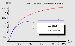
Figure 1: Common leading behaviour.

Note that the MPF model saturates before the Amdahl model under these conditions and it therefore predicts a smaller overall capacity than the Amdahl model.

Alternatively, we could consider the other extreme shown in Figure 2 where both models approach the same asymptote at for large multiprocessor configurations.

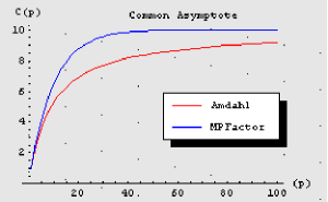
Figure 2: Common asymptote.

Now, the faster saturation of the MPF model means that maximal capacity is reached at smaller configurations than predicted by the Amdahl model.

We take the position that such questions should be addressed on purely physical grounds, otherwise, multiprocessor capacity predictions are reduced to an exercise in mere curve fitting. The problem is that no consistent physical interpretation of these parametric models exists.

Elsewhere [16], this author has shown how these parametric scaling models could be expanded as a finite series in which each term has a distinct pictorial representation. This led to the conclusion that (1) can be regarded as representing a “broadcast” protocol while (2) can be regarded as representing a “bucket brigade” protocol [17]. The latter is a less than satisfactory because it appears quite unphysical when compared to the way actual multiprocessor systems operate.

In this paper, we present a more consistent interpretation based on queueing models. The usual difficulty with modeling multiprocessors as elementary queues (e.g., M/M/m) is that they do not account for “interference” effects between the processors (the so-called multiprocessor effect). We shall overcome this limitation in two distinct ways:

1. Multiprocessor Speedup will be identified with a bus-oriented M/M/1//p queueing model where processor interference is represented as communication delays across the bus.

2. The Multiprocessing Factor will be identified with a processor-oriented M/G/1 model representing the run-queue where multiprocessor interference is associated with a staged service distribution.

Single class workloads are assumed throughout since that will prove sufficient for the analysis of (1) and (2).

Just as queueing delays for elementary queues can have vastly different analytic forms (assuming a closed analytic form exists), it would be useful to select the parametric sizing model on the basis of the underlying queueing dynamics along the lines indicted earlier for the sizing of buffers.

2 Multiprocessor Scalability

We begin by briefly reviewing the conventional intuition behind the single parameter sizing models in (1) and (2).

2.1 Multiprocessor Speedup

Amdahl’s law [1] is well-known and frequently cited in the context parallel processing performance ([4], [18], [19]) where is it also known as the speedup ([3], [2]). The underlying notion is that for a fixed workload size there is a fraction $\sigma\in(0,1)$ of the workload for which the execution time remains constant as p increases. Ultimately, this fraction dominates the speedup function causing it to become sublinear.

In the subsequent queueing analysis, it will be more useful to use the dual representation of processing capacity based on relative throughput or scaleup [17]:

$$C(p)=\frac{X(p)}{X(1)}$$ (3)

(3) is reflective of the motivation for selling multiprocessors that support commercial applications. There, the goal is to accommodate incremental user growth through the purchase of increased processor capacity while minimizing the degradation to single user responsiveness.

Assume the number of users (N) per processor is fixed (i.e., $N/p=const.$). Let $R_{1}$ be the mean response time experienced by N users on a single processor. We would like to maintain the response times at $R_{1}$ but adding another processor with N users (now 2N total users across 2 processors), we find $R_{2}>R_{1}$ due to the multiprocessor effect.

Defining the number of completed transactions per processor as c, the uniprocessor throughput is $X(1)=c/R_{1}$. For 2 processors, the throughput becomes $X(2)=2c/R_{2}$ where the response time $R_{2}$ with 2 processors is sightly longer than $R_{1}$ by a fractional amount $\sigma~{}R_{1}$. In other words, $X(2)=2c/(1+\sigma)R_{1}$. For 3 processors we have $X(3)=3c/(1+2\sigma)R_{1}$.

Generalizing to p processors, the throughput is $X(p)=p~{}c/R_{p}$ where $R_{p}=R_{1}+(p-1)~{}\sigma R_{1}$ accounts for the fractional increase in response time due to the activity of users on other (p - 1) processors. Substituting $X(1)$ and $X(p)$ into (3) produces:

$$C(\sigma,p)=\frac{p~{}c}{T_{p}}~{}\frac{R_{1}}{c}=\frac{p~{}R_{1}}{R_{1}~{}+~{}(p-1)~{}\sigma~{}R_{1}}$$ (4)

which, after the elimination of $R_{1}$, is identical to (1). The asymptotic capacity is:

$$\lim_{p\rightarrow\infty}C(\sigma,p)=\frac{1}{\sigma}$$ (5)

The reason that the expressions for the speedup in (1) and the scaleup in (4) are identical (i.e., duals of each other) follows from:

$$\frac{(1-\sigma)/p}{\sigma}=\frac{(1-\sigma)}{p\sigma}$$

The key quantity that determines the sublinear capacity is the ratio of the “parallel” portion $(1-\sigma)$ to “serial” portion $\sigma$ of the workload. With respect to that ratio, it is inconsequential whether the parallel portion is scaled down by p or the serial portion is scaled up by p. The effect on the ratio is the same.

2.2 Multiprocessing Factor

The multiprocessing factor (MPF) is intended as a measure of how much effective processor capacity is available (or lost) as more processors are added to the backplane.

Figure 3: Different MPF factors.

Consider a workload running on a uniprocessor that has a measured throughput of X(1) = 100 transactions per second (TPS). When run on a dual processor the aggregate throughput is measured as X(2) = 180 TPS. Since X(2) is less than double X(1), this loss can be expressed as: $180=(1+\phi)100$ TPS, where the quantity $\phi=0.8$ is the MPF. The second processor only contributes 80 percent of the capacity of the first processor. Continuing along these lines, a third processor would only be expected to contribute 80% of the second processor i.e., 64 TPS. The aggregate throughput being: $X(3)=X(1)+\phi X(1)+\phi(\phi X(1))$ = 244 TPS.

Generalizing this cumulative procedure and applying the definition in (3) produces:

$$C(\phi,p)=1~{}+~{}\phi~{}+~{}\phi^{2}~{}+~{}\ldots~{}+~{}\phi^{p-1}$$ (6)

which is equivalent to (2) for $\phi<1$ since it is a finite geometric sum. The asymptotic capacity is:

$$\lim_{p\rightarrow\infty}C(\phi,p)=\frac{1}{1-\phi}$$ (7)

If $\phi=1$ (no MPF), then

$$C(1,p)=\sum_{k=0}^{p}~{}\phi^{k}\equiv p$$ (8)

which is a linear rising function representing ideal multiprocessor scalability.

For the purposes of comparison, (1) can also be written as a finite series

$$C(\sigma,p)=1~{}+~{}A_{1}~{}+~{}A_{2}~{}+~{}\ldots~{}+~{}A_{p-1}$$ (9)

where

$$A_{i}=\frac{1-\sigma}{1+\sigma~{}(p-1)},~{}~{}i=1,2,\ldots,(p-1).$$

Unfortunately, (9) is not a power series like (6), so the choice of scaling equation is not obvious even in a series representation. Other ambiguities persist. (1) and (2) could be matched either at leading order by setting $C(\sigma,1)=C(\phi,1)$ as shown Figure 1 or they could be matched asymptotically by setting $\sigma=(1-\phi)$ as shown Figure 2.

3 Queueing Dynamics

In this section, we develop queueing models to resolve the ambiguities described above.

3.1 Bus-oriented Model

The bus-oriented model comprises a closed queueing network, or Repairman model [21], containing a finite number (p) of requests and K queueing centers (K = 1 repair station and mean service demand D will be sufficient for our discussion).

Figure 4: Repairman model.

The requests can be thought of as memory references [22] issued by p processors each of which executes in “parallel” for a mean time (Z). The queueing center represents a “serial” bus or other interconnect network [23] by which the processors can communicate or transfer data. Typically, we expect $D~{}\ll~{}Z$ to hold because the mean execution periods should exceed the mean transit times across the bus.

System throughput (X) and communication latency (R) are related by:

$$X(p)=\frac{p}{R(p)+Z}$$ (10)

The saturation bound $X_{max}=1/D$ represents the maximum throughput the multiprocessor can achieve.

3.1.1 Synchronous Requests

The worst case bound [24] on multiprocessor throughput ($X_{min}$) occurs when all p processors issue synchronous communication requests. Then $R(p)=p~{}D$ (maximal queueing) and (10) becomes:

$$X_{sync}(p)=\frac{p}{pD+Z}$$ (11)

Using the definition in (3), we can use (11) to write:

$$C_{sync}(p)=\frac{p~{}(D+Z)}{pD+Z}=\frac{p}{p\left(\frac{D}{D+Z}\right)+\left(\frac{Z}{D+Z}\right)}$$ (12)

Rearranging terms and simplifying produces:

$$C_{sync}(p)=\frac{p}{(p~{}-~{}1)\left(\frac{D}{D+Z}\right)+1}$$ (13)

We immediately recognize (13) as a version of (1)

Figure 5: Capacity of the Repairman and Amdahl models.

where the parameter $\sigma$ is now identified with the queueing parameters D and Z via the ratio:

$$\sigma=\frac{D}{D+Z}$$ (14)

The range of values for $\sigma$ in (14) evidently corresponds to:

1. $\sigma\rightarrow 0$ as $D\rightarrow 0$ (zero latency)

2. $\sigma\rightarrow 1$ as $Z\rightarrow 0$ (zero execution)

(14) establishes that $C_{sync}(p)$ in (13) is identical to $C(\sigma,p)$ in (1). Although the queue-theoretic bound (11) on throughput is known [24], its relationship to the Amdahl scaleup (4) seems not to have been discussed in the literature.

The bus-oriented queueing model also supports an earlier conclusion [16], [17] that Amdahl’s law can be interpreted as representing a kind of “broadcast protocol” where all execution simultaneously halts while processors exchange messages across the communication fabric.

3.1.2 Response Times

The general response time for the Repairman model in Fig. (4) is given by:

$$R(p)=\frac{p}{X(p)}-Z$$ (15)

The response characteristics for the bus-oriented model can be determined by substituting (11) into (15) and simplifying:

$$R_{sync}(p)=p~{}D$$ (16)

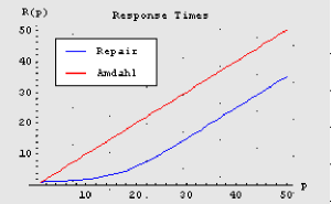
Figure 6: Response characteritics of the Repairman and Amdahl models.

We see that the relative response time

$$\frac{R_{sync}(p)}{R_{sync}(1)}=p$$ (17)

corresponding to the Amdahl bound is a linear function of p (Fig.  6) and independent of $\sigma$ because the system is already in severe saturation due to synchronized queueing.

3.2 Processor-oriented Model

The Coxian distribution [21] represents a type of composite server (see Fig. 7)  [22], [24] with staged exponentially distributed service rates $\mu_{i}$ for i = 1,2, …, p stages, and probability

$$A_{i}=\prod_{i=0}^{p-1}~{}a_{i},$$

of advancing to the $i^{th}$ server and branching probability $b_{i}$ of exiting after the $i^{th}$ server. The next request cannot enter the service facility until the current request has either completed all stages or exited after the $i^{th}$ stage. Consequently, there is no queueing at any of the Coxian stages.

Figure 7: Coxian server.

The expected service time (first moment) is:

$$E\{S\}=\sum_{i=1}^{p}~{}A_{i}b_{i}\left(\prod_{j=1}^{i}~{}\frac{1}{\mu_{j}}\right)$$ (18)

with variance:

$$Var\{S\}=E\{S^{2}\}-E^{2}\{S\}$$ (19)

where the second moment is given by:

$$E\{S^{2}\}=\sum_{i=1}^{p}~{}A_{i}b_{i}\left[\left(\prod_{j=1}^{i}~{}\frac{1}{\mu_{j}^{2}}\right)+\left(\prod_{j=1}^{i}~{}\frac{1}{\mu_{j}}\right)^{2}\right]$$ (20)

A well-known [21] special case is the Erlang-k distribution where all $\mu_{i}=\mu$ and all $b_{i}=0$ and squared coefficient of variation $C^{2}\{S\}=1/p$ [25].

3.2.1 Uniform Coxian

The special case of interest to us is, $\mu_{i}=\mu$, $a_{i}=\phi$ with $a_{p}=0$ and $b_{i}=1-\phi$ with $b_{0}=0$. We shall refer to this as a uniform Coxian distribution. Then (18) reduces to:

$$E\{S\}=\frac{1}{\mu}+\frac{\phi}{\mu}+\frac{\phi^{2}}{\mu}+\dots+\frac{\phi^{p-1}}{\mu}$$ (21)

Using Little’s law $U=\lambda E\{S\}$, (21) can be rewritten as:

$$U(\phi,p)=\frac{\lambda}{\mu}~{}\left(\frac{~{}1-\phi^{p}}{1-\phi}\right)$$ (22)

Since $U(\phi,p)\geq 1$, (22) represents the total utilization of the uniform Coxian service facility. It is bounded above by

$$U(\phi,p)\leq\frac{\rho}{1-\phi}$$

where $\rho=\lambda/\mu$. Moreover, (2) can now be expressed in terms of (22) as:

$$\rho~{}C(\phi,p)=U(\phi,p)$$ (23)

Hence, the MPF capacity model presented in section 2 can also be interpreted as the total utilization of a p-stage uniform Coxian server. For a single-stage server p = 1 and (23) reduces to $U(\phi,1)=\rho$, as expected.

In this queueing model, the finite geometric series in (6) arises from the branching process within the service center (not the arrivals process). This branching represents the loss of service after some number of processor cycles due to system overhead. The total utilization $U(\phi,p)$ corresponds to the average impact of that loss.

3.2.2 Response Times

The corresponding response times (Fig. 8) for the uniform Coxian model can be calculated as an M/G/1 queue using the Pollacek-Khintchine formula [25]:

$$R(\phi,\rho)=E\{S\}\left[1~{}+~{}\frac{\rho~{}(1+C_{\phi}^{2}\{S\})}{2~{}(1-\rho)}\right]$$ (24)

where the squared coefficient of variation

$$C_{\phi}^{2}\{S\}=\frac{Var\{S\}}{E^{2}\{S\}}$$

is defined in terms of (18) and (20) and lies in the range $1/p<C_{\phi}^{2}\{S\}<1$. As expected, the uniform Coxian model represents a hypoexponential server. The variance in the service time is smaller than it would be for an M/M/1 queue.

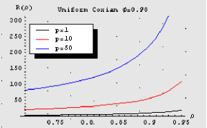
Figure 8: Response time $R(\rho)$ as a function of $\rho$.

The response time (24) is plotted as a function of $\rho$ in figure (8) for a fixed value of $\phi$. It has the typical characteristic expected of an open class queue. With only a single stage and probability 1 of advancement ($\phi=0.98$) $R(\rho)$ is close to an M/M/1 queue since $C_{\phi}^{2}\{S\}\sim 1$. As more stages are added, the response time at any load $\rho$ increases as shown by the curves for p = 10 and p = 50. Note, however, that the progressive increase at that load becomes smaller as the number of stages increases. This effect can be seen more clearly in figure (9) which shows response times plotted as a function of p for a fixed load $\rho=0.75$ up to 100 stages representing a large-scale multiprocessor. A surprising feature, for modeling multiprocessors, is that the response time characterisitcs are sublinear for all $\phi<1$. Contrast this with the response time characterisitcs in figure (6).

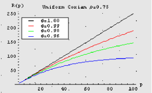
Figure 9: Response time $R(p)$ vs. the number of stages for $\rho=0.75$.

Only for the special case $\phi=1$ (Erlang-p), does the response time increase linearly because there, all the processor work is accounted for i.e., $U(\phi,p)=p\rho$. That case, however, is tantamount to linear scalability in (8) which ignores the MP effect and is therefore of little value for multiprocessor sizing.

The queue-theoretic attributes of the MPF model can be summarized as follows:

1. Only one request at a time can enter the Coxian server.

2. Multiprocessor overhead is treated as a probabilistic loss of work.

3. Processor utilization due to the MP effect is unaccounted for.

4. Service periods are hypo-exponential.

5. Response times become sublinear with an increasing number of processors.

These characteristics appear counter-intuitive as a model of multiprocessor scalability.

4 Conclusions

Based on our queueing analysis of these multiprocessor models we are now in a position to say something about the applicability of the bus-oriented (Amdahl) model defined by (1) and the server-oriented model (MPF) model defined by (2).

If matched at small processor configurations, both capacity models are essentially indistinguishable when fitted to benchmark data. As configurations become larger, however, the MPF model becomes pessimistic relative to the Amdahl model. This appears contradictory when we recall that Amdahl scaling corresponds to the worst-case bound of the more constrained closed queueing model.

Capacity scaling for the bus-oriented (Amdahl) model in section 3.1 is an explicit function of the system throughput X(p). Response times for bus-oriented (Amdahl) model will have the classic “hockey-stick” shape due to the negative feedback effects of a finite number of requests in the closed queueing network. Such response time curves are associated with the constraint that no more than one bus request per processor can be outstanding. Utilizations of both the bus, U(p), and the processors, Z.X(p), are accounted for explicitly.

Based on the discussion in section 3.2, the relative capacity for server-oriented model (MPF) model is equivalent to the total utilization U(p) of a p-stage Coxian server. For a given value of $\phi$, the total utilization becomes sublinear with increasing stages because the likelihood diminishes that a request will visit all stages. In this model, multiprocessor overhead is treated as a loss of serviceable work.

Considered as an M/G/1 queue, the multiprocessor is represented as a single Coxian server with processor interference accounted for by the variance in the service period. That only one request can enter the Coxian server at a time is already unrealistic for a model of a multiprocessor but a variance in the service periods that is less than an exponential server (i.e., hypoexponential), seems contradictory to expectations for a model of the multiprocessor effect. M/G/1 queues with $C^{2}\{S\}\gg 1$ (i.e., non-Coxian) have been used to model disk storage and token ring networks [25], however, we need the Coxian stages to account for the geometric series in (2).

A hyperexponential Coxian would also produce higher variance $C^{2}\{S\}>1$ in the service periods but it is well known ([21], [25]) that just a few parallel stages are sufficient for that and thus p could no longer be associated explicitly with the number of processors. Moreover, and hyper-exponential Coxian does not produce a mean service time that has the geometric series required to account for (2).

The response time for the Coxian server model becomes sublinear as the processor configuration is expanded. This is unlikely to be seen in benchmark measurements of real multiprocessors. Such an unphysical effect follows from the fact that the utilization due to lost processor work is unaccounted for in the Coxian model. In reality, one expects multiprocessor overhead to be accrued as processor kernel time rather than processor user time. The total processor utilization is the sum of both contributions but the uniform Coxian server does not account for kernel time in the workload.

Finally, we suggest that neither of the models considered here is truly sufficient as a general model of multiprocessor scalability. Elsewhere, we have already proposed a two-parameter model [26]:

$$C(\alpha,\beta,p)=\frac{p}{1+\alpha~{}[(p-1)+\beta~{}p~{}(p-1)]}$$ (25)

in which the $\alpha$ parameter is identified with queueing delays and the $\beta$ parameter with additional delays due to pairwise coherency [27] mismatches [17]. The latter induces retrograde throughputs C($\alpha$, $\beta$, p) $\rightarrow$ 1/p as p $\rightarrow\infty$ that are indeed seen in multiprocessor capacity measurements [28]. Retrograde throughput cannot be modeled parametrically using either (1) or (2) nor can it be represented using conventional queueing theory without the introduction of load-dependent servers such that $E\{S\}\sim 1/p$. In the limit where coherency penalties vanish ($\beta=0$), (25) reduces to the Amdahl model (with $\alpha=\sigma$) in (1). As we have demonstrated here, Amdahl’s law has a natural physical interpretation as synchronous queueing within a Repairman model. The two-parameter function (25) can be viewed as a load-dependent extension of that queueing dynamics.

Although we have been able to show that the MPF scaling equation (2) belongs to an M/G/1 queueing model with a load-dependent Coxian server, that load dependence is not of the correct type for modeling multiprocessor overhead because it gives rise to unphysical effects. We therefore caution against its use for large-scale multiprocessor servers.

References

- [1] G. Amdahl. “Validity of the single processor approach to achieving large scale computing capabilities”. Proc. AFIPS Conf., 30:483–485, Apr. 18–20 1967.
- [2] J. L. Hennessy and D. A.Patterson. Computer Architecture: A Quantitative Approach. Morgan Kaufmann, 2nd. edition, 1996.
- [3] E. Gelenbe. Multiprocessor Performance. Wiley, 1989.
- [4] W. Ware. “The ultimate computer”. IEEE Spectrum, pages 89–91, March 1982.
- [5] H. P. Artis. “Quantifying multiprocessor overheads”. Proc. CMG Conference, pages 363–365, 1991.
- [6] A. Cockcroft and W. Walker. Sun Blueprints: Capacity Planning for Internet Services. Prentice–Hall, New Jersey, 2000.
- [7] J. W. McGalliard. “Case study of table-top sizing with workload-specfic estimates of the multiprocessor effect”. Proc. CMG Conference, Nashville, Tennesee:208–217, December 1995.
- [8] J. L. Fitch. “A guide for performance and capability validation”. Document KMP–94–2–P, U.S. General Services Administration, 1993.
- [9] W. Bitner. “VM/ESA greater N–way thoughts”. http://www.vm.ibm.com/devpages/bitner/presentations/vmnway.html #Section_0.6, October 1996.
- [10] Hitachi Data Systems Inc. “Hitachi unleashes new series of e–Business mega servers with world’s highest performance and availability”. http://al.hds.com/news/000207.html, 2000.
- [11] David Floyer. “The performance and price/performance of current mainframe systems”. http://www.unisys.com/hw/servers/clearpath/16222.htm, May 1998.
- [12] IBM. “Large systems performance reference”. http://www-1.ibm.com/servers/eserver/zseries/lspr/, February 2002.
- [13] System Performance Evaluation Corporation SPEC. “CPU2000 benchmark”. http://www.spec.org/osg/cpu2000/, 2000.
- [14] Transaction Processing Performance Council TPC. “TPC–C benchmark”. http://www.tpc.org/tpcc/, 2000.
- [15] Transaction Processing Performance Council TPC. “TPC–W benchmark”. http://www.tpc.org/tpcw/, 2000.
- [16] N. J. Gunther. “Understanding the MP effect: Multiprocessing in pictures”. Proc. CMG Conference, San Diego, California:957–968, December 1996.
- [17] N. J. Gunther. The Practical Performance Analyst. iUniverse.com, Inc., Lincoln, Nebraska, Print-On-Demand edition, 2000.
- [18] H. P. Flatt. “Further results using the overhead model for parallel systems”. IBM J. Res Develop., 35(5/6):721–726, 1991.
- [19] A. H. Karp and H. P. Flatt. “Measuring parallel processor performance”. Comm. ACM, 33(5):539–543, 1990.
- [20] J. L. Gustafson. “Reevaluating Amdahl’s law”. Comm. ACM, 31(5):532–533, 1988.
- [21] A. O. Allen. Probability, Statistics, and Queueing Theory with Computer Science Applications. Academic Press, San Diego, 2nd. edition, 1990.
- [22] M. Ajmone-Marsan, G. Balbo, and G. Conte. Performance Models of Multiprocessor Systems. MIT Press, Cambridge, Mass., 1990.
- [23] D. E. Culler, R. M. Karp, D. Patterson, A. Sahay, E. E. Santos, K. E. Schauser, R. Subramonian, and T. Eicken. “LogP: A practical model of parallel computation”. Comm. ACM, 39(11):79–85, November 1996.
- [24] E. D. Lasowska, J. Zahorjan, G. S. Graham, and K. C. Sevcik. Quantitative System Performance: Computer System Analysis Using Queueing Network Models. Prentice–Hall, Engelwood Cliffs, 1984.
- [25] P. G. Harrison and N. M.Patel. Performance Modelling of Communication Networks and Computer Architectures. Addison–Wesley, Wokingham, U. K., 1993.
- [26] N. J. Gunther. “A simple capacity model for massively parallel transaction systems”. Proc. CMG Conference, San Diego, California:1035–1044, December 1993.
- [27] S. Cho and G. Lee. “Reducing cache coherence overhead in shared–bus multiprocessors”. Proc. EURO–PAR’96, August 1996.
- [28] N. J. Gunther. “Performance and scalability models for a hypergrowth e-Commerce Web site”. In R. Dumke, C. Rautenstrauch, A. Schmietendorf, and A. Scholz, editors, Performance Engineering: State of the Art and Current Trends, volume # 2047, pages 267–282. Springer–Verlag, Heidelberg, 2001.