Cellular automata and communication complexity

Abstract

The model of cellular automata is fascinating because very simple local rules can generate complex global behaviors. The relationship between local and global function is subject of many studies. We tackle this question by using results on communication complexity theory and, as a by-product, we provide (yet another) classification of cellular automata.

1 Introduction

The model of cellular automata was invented in the 1950’s mostly by von Neumann as a tool to study self-reproduction (see [vN67]). It was then meant both as a tool to model real life dynamical systems and as a model of an actual computer. Since then cellular automata are studied theoretically either as a model of massive parallel computation or as a discrete dynamical system. They are also studied experimentally either as a tool to model complex natural systems ranging from economy, geology, biology, chemistry, sociology, etc or as a framework to do simulations. For a general introduction, see [DM99].

A cellular automaton is an infinite and discrete grid of cells. Each cell contains at every time step a particular state from a finite set. The cell state obeys a local rule, mapping its state and the state of the neighborhood to a new cell state. This rule is applied uniformly and synchronously to all cells of the grid. So the local rule generates a global mapping on grid configurations, which can be quite complex. For example, some simple local rules give computation universal cellular automata.

It is an important issue to understand the relationship between local and global mappings. In this paper we view a cellular automaton as a grid of communicating cells. During the evolution information can flow through the whole grid. In one-dimensional cellular automata a fixed cell divides the grid into two parts and we are interested in the way information flows through the cell. By studying the communication complexity of successive iterations of the local function we provide a new way to look at the global behavior of cellular automata.

2 Elementary cellular automata and $0-1$ matrices

In this paper we mainly focus on elementary cellular automata (ECA) which we define hereafter, although generalization to any one-dimensional cellular automata (CA) is always possible and quite straightforward.

We consider the one-dimensional cellspace, where each cell can be either in state $0$ or in state $1$. An ECA is defined by a local function ${f:\{0,1\}^{3}\rightarrow\{0,1\}}$ which maps the state of a cell and its two immediate neighbors to a new cell state. There are exactly $2^{2^{3}}=256$ ECA and each of them is is identified with its Wolfram number, which is between 0 and 255 and defined as

$$\sum_{a,b,c\in\{0,1\}}(4a+2b+c)f(abc).$$

Following the cellular automata’s paradigm, all the cells change their states synchronously according to the local function. This endows the line of cells with a global dynamics whose links with the local function are still to be understood in the general case as already pointed out in the introduction. Let us remark however that some simple transformations on the local function induce simple transformations on the global dynamics: the space-symmetric ECA of $f$ is the ECA $f^{\prime}$ with ${f^{\prime}(a,b,c)=f(c,b,a)}$ and the state-symmetric is the ECA $f^{\prime\prime}$ with ${f^{\prime\prime}(a,b,c)=\overline{f(\bar{a},\bar{b},\bar{c})}}$. Thus we consider only ECA whose Wolfram number is minimal among its symmetries. This leaves 88 out of 256 ECA to consider, which is more than 256/4 because some ECA are symmetric.

To tackle the issue of local/global relationships, we study the evolution of one cell’s state after finitely many time steps. Given that after $n$ time steps the value of a cell depends on its own initial state and the initial states of the $n$ immediate left and $n$ immediate right neighbor cells, we define the $n$-th iteration of $f$, ${f^{n}:\{0,1\}^{2n+1}\rightarrow\{0,1\}}$, as ${f^{1}=f}$ and for ${n\geq 2}$ as

$$\begin{split}f^{n}(x_{-n},\dots,x_{-1},x_{0},x_{1},\dots,x_{n})=f\bigl{(}&f^{n-1}(x_{-n},\dots,x_{n-2}),\\ &f^{n-1}(x_{-n+1},\dots,x_{n-1}),\\ &f^{n-1}(x_{-n+2},\dots,x_{n})\bigr{)}.\end{split}$$

Notice that knowing a simple description of $f^{n}$ for arbitrary $n$ is knowing the long term (asymptotic) behavior of the whole line of cells.

We therefore propose to measure the complexity of an ECA $f$ by the asymptotic complexity of the functions $\bigl{(}f^{n}\bigr{)}$. For that purpose, $0-1$ matrices reveal themselves to be a striking representation. When fixing the state of the central cell among ${2n+1}$ adjacent ones to $0$ for instance, $2^{2n}$ initial configurations are possible each leading the central cell to a peculiar state after $n$ time steps. This can be summarized in a square matrix $M_{0}^{n}$ of size $2^{n}$ defined as follows:

$$M_{0}^{n}(i,j):=f^{n}(\stackrel{{\scriptstyle\leftarrow}}{{b_{i}}},0,b_{j})$$

where $b_{k}$ is the binary representation of the integer $k$ on exactly $n$ bits, and $\stackrel{{\scriptstyle\leftarrow}}{{b_{k}}}$ its reverse representation. Each value $n$ defines a different matrix, and we have, for each ECA, an infinite family of binary matrices for $n=1,2,\ldots$.

Note that the definition of $M_{0}^{n}$ is unique up to permutation of rows and columns. We could as well have defined $\tilde{M}_{0}^{n}(i,j):=f^{n}(b_{i},0,\stackrel{{\scriptstyle\leftarrow}}{{b_{j}}})$ for example.

Fixing the center cell to $0$ was arbitrary. We could as well have chosen $1$. Therefore, any ECA $f$ defines two families of binary matrices (see figure 1). Note that the first matrix of each family, standing for ${n=1}$, defines completely the local function. One can think of these matrices as seeds for the families.

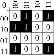
n= 1 2 … n= 1 2 3 4 5 … c=0 … … c=1 … …

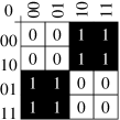
Figure 1: The two families of binary matrices $M_{c}^{n}$ of Wolfram rule 54 cellular automata

The matrices can in some cases ease the understanding of the global behavior. In figure 2 we show the space time diagram of rule 105 for some arbitrary configuration, and on the right the matrix $M_{0}^{5}$. In contrast with the space-time diagram, the matrix looks simple, and indeed there is a small description of the additive rule 105 (which is given later in the paper). We should emphasize that the space-time diagram shows the evolution of only a single configuration, while the matrix covers all configurations.

         

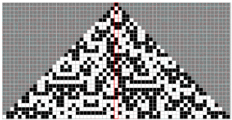
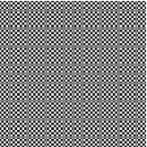
Figure 2: A space time diagram for rule 105 (left) and one matrix of its families (right). In the diagram every row is a configuration and time goes upward. It shows only those cells, on which the upper center cell depends.

Different measures on the matrices are possible in order to analyze the underlying ECA. Among them we choose the simplest one: the number of different rows. To be precise we define $d_{n}$ as the maximum of the $4$ following integers: number of different rows of $M_{0}^{n}$, number of different columns of $M_{0}^{n}$, number of different rows of $M_{1}^{n}$, number of different columns of $M_{1}^{n}$.

3 Experimental measuring

Since the family of matrices of a given ECA defines the global and long term behavior, we can express $d_{n}$ as a known function of $n$ only once we understood the global behavior. However in some cases, seeing the matrices helped us to understand the global function.

We did brute force computations in order to compute $d_{n}$ for $n\in\{1,\ldots,12\}$ and for all ECAs. The complete results are shown in the web page www.lri.fr/~durr/CACC/. Figure 3 plots $d_{n}$ for different rules. We obtain quite different sequences, which we classify as follows:

Bounded:

there is ${b\in\mathbb{N}}$ such that ${\forall n\ :\ d_{n}\leq b}$.

Linear:

there are values ${a_{0}\in\mathbb{N}}$ and ${a_{1}\in\mathbb{Q}}$ such that $d_{n}=\lfloor a_{1}n\rfloor+a_{0}$, for all $n\geq n_{0}$ for some fixed value $n_{0}$.

Other:

in this class we put rules where non of above applies. In some cases $d_{n}$ seems to be bounded by a polynomial in $n$, and in some cases $d_{n}$ seems to be exponential.

Figure 3: Different sequences $d_{n}$.

We want to emphasize that this classification is mainly experimental. Most of the time we don’t have mathematical evidence for determining whether a rule belongs to one class rather than to another. Table 1 shows the classification of all rules (again, only up to symmetric transformations which preserve $d_{n}$).

The following sections are devoted to the few ECA where we were able to give a closed formula for $d_{n}$ making their classification rigorous.

Bounded:

0, 1, 2, 3, 4, 5, 7, 8, 10, 12, 13, 15, 19, 24, 27, 28, 29, 32, 34, 36, 38, 42, 46, 51, 60, 71, 72, 76, 78, 90, 105, 108, 128, 130, 136, 138, 140, 150, 154, 156, 160, 170, 172, 200, 204

Linear:

11, 14, 23, 33, 35, 43, 44, 50, 56, 58, 77, 132, 142, 152, 168, 178, 184, 232

Other:

6, 9, 18, 22, 25, 26, 30, 37, 40, 41, 45, 54, 57, 62, 73, 74, 94, 104, 106, 110, 122, 126, 134, 146, 164

Table 1: A classification of ECAs

4 Communication complexity

The communication complexity framework appears as an extremely useful tool for calculating $d_{n}$. The communication complexity theory studies the information exchange required by different actors to accomplish a common computation when the data is initially distributed among them. To tackle that kind of questions, A.C. Yao [Yao79] suggested the two-party model: two persons, say Alice and Bob, are asked to compute together the values taken by a function $f$ of $2$ variables ($x$ and $y$ taking values in a finite set), Alice always knowing the value of $x$ only and Bob that of $y$ only. Moreover, they are asked to proceed in such a way that the cost — the total number of exchanged bits — is minimal in the worst case. Now different restrictions on the communication protocol lead to different communication complexity measures.

Definition 1 (Many round communication complexity).

The many round communication complexity $CC(f)$ of a function $f$ is the cost of the best protocol for $f$.

Definition 2 (One-way communication complexity).

A protocol is AB-one-way if only Alice is allowed to send information to Bob, and Bob has to compute the function solely on its input, and the received information. The AB-one-way communication complexity is the worst case number of bits Alice needs to send. BA-one-way complexity is defined in the same manner. Finally, the one-way complexity $C(f)$ of $f$ is the maximum of its AB-one-way and BA-one-way complexities.

Whereas most studies concern the many round communication complexity, we focus only on the one-way communication complexity. In terms of cellular automata it will permit us to measure the amount of information which have to flow from one side to another. Also from a practical point of view, the former measure is extremely difficult to compute for most functions, while the last measure is quite easy as shown by the next fact.

Fact 3 ([KN97]).

Let $f$ be a binary function of ${2n}$ variables and $M_{f}\in\{0,1\}^{2^{n}\times 2^{n}}$ its matrix representation, defined by $M_{f}(x,y)=f(xy)$ for $x,y\in\{0,1\}^{n}$. Let $d(M_{f})$ be the maximum of the number of different rows and the number of different columns in $M_{f}$. We have

$$C(f)=\left\lceil\log_{2}\bigl{(}d(M_{f})\bigr{)}\right\rceil.$$

Proof.

Let be a AB-one-way protocol, where Alice knows $x\in\{0,1\}^{n}$ and Bob $y\in\{0,1\}^{n}$. Suppose Alice sends to Bob at most $k$ bits which depend solely on $x$, say by some mapping ${g:\{0,1\}^{n}\rightarrow\{0,1\}^{k}}$. Then since Bob knows $f(x,y)$ only from $y$ and $g(x)$, we must have $f(x,y)=f(x^{\prime},y)$ for all $x,x^{\prime}$ with $g(x)=g(x^{\prime})$. In terms of matrix representation it means that the rows in $M_{f}$ indexed by $x$ and $x^{\prime}$ are the same. So we must have ${k\geq\left\lceil\log_{2}\bigl{(}d(M_{f})\bigr{)}\right\rceil}$.

Conversely, ${\left\lceil\log_{2}\bigl{(}d(M_{f})\bigr{)}\right\rceil}$ are sufficient for Alice: knowing $M_{f}$ she only has to say to Bob the group of identical rows the current entry belongs to. ∎

Then, up to a $\log$ transformation, the complexity measure $d_{n}$ appears to be precisely the exchanged information amount required for Alice and Bob to compute $f^{n}$ when Alice has the $n$ left cells and Bob has the $n$ right cells, both knowing the value of the central cell and maximizing over the scenario where only Alice is allowed to talk, and the scenario where only Bob is allowed to talk.

5 ECA with bounded complexity

We will now give formal proofs for some ECA to be in the bounded complexity class.

Definition 4.

An ECA is nilpotent if it converges to a unique configuration from any initial configuration in finite time.

Given that an ECA $f$ is nilpotent if and only if there is $n_{0}$ such that $f^{n}$ is constant for all $n\geq n_{0}$, it is clear that a nilpotent ECA will have $d_{n}=1$ for large enough $n$: no communication is needed between Alice and Bob to compute the final state of the central cell.

There is a natural condition generalizing nilpotency, which can be used to prove bounded complexity for ECA.

Definition 5.

An ECA $f$ has a limited sensibility if the number of cells $f^{n}$ actually depends on is bounded by a constant independent of $n$. Formally there is a constant $c$ such that $\forall n$ $\exists w\in\{0,1\}^{2n+1}$ with $\sum_{i=1}^{2n+1}w_{i}\leq c$ and $f^{n}(u)=f^{n}(u\wedge w)$ for all $u\in\{0,1\}^{2n+1}$ where $\wedge$ is the bitwise boolean and.

The ECA has half-limited sensibility if the condition above holds for the weaker condition $\sum_{i=1}^{n}w_{i}\leq c$ or equivalently $\sum_{i=n+1}^{2n+1}w_{i}\leq c$.

Clearly if $f$ has limited sensibility $c$ at most $c$ bits need to be exchanged between Alice and Bob. We show now that the half-limited sensibility is enough to achieve bounded one-way communication complexity.

Lemma 6.

An ECA with half-limited sensibility is in the bounded complexity class.

Proof.

Without loss of generality, let us assume that Alice knows the left cells and that the sensibility of $f^{n}$ is limited by $c$ on the first $n$ cells. There is a trivial AB-one-way protocol of cost $c$. We give a BA-one-way protocol of cost $2^{c}$, which is worse but still constant. Bob successively guesses each possible value of Alice’s sensible cells and sends the list of the corresponding values for $f^{n}$. Then Alice select among this list, the entry corresponding to the actual values of its sensible cells. ∎

An interesting example is rule 60. It has sensibility $0$ on the second half, and unlimited sensibility on the first half, as it computes the parity of the first $n+1$ cells, whenever $n+1$ is a power of $2$.

Unfortunately, it is undecidable to determine whether a given CA has a limited sensibility (by reduction from the nilpotency problem which is undecidable [Kar92]). Except some particular examples, we can only guess if a ECA has limited sensibility based on brute force computation for small values of $n$.

However there is a decidable property, which is sufficient for a ECA to be in the bounded class.

Definition 7.

An ECA $f$ is additive is there are binary operators $\oplus$ and $\otimes$ (not necessarily distinct), and a neutral element $e$ such that for all $x$, ${x\oplus e=e\oplus x=x}$ and with

$$\forall x,y,z,x^{\prime},y^{\prime},z^{\prime}\quad\left\{\begin{aligned} f(x\oplus x^{\prime},y\oplus y^{\prime},z\oplus z^{\prime})&=f(x,y,z)\otimes f(x^{\prime},y^{\prime},z^{\prime})\\ f(x\otimes x^{\prime},y\otimes y^{\prime},z\otimes z^{\prime})&=f(x,y,z)\oplus f(x^{\prime},y^{\prime},z^{\prime})\end{aligned}\right.$$

Remark.

The previous definition can naturally be extended to longer operator chains. However, as far as ECA are concerned, $2$ operators are sufficient to capture all additive rules.

Additivity is preserved by iterations of the local rule, as stated in the following lemma which can be proved straightforwardly by induction on $n$.

Lemma 8.

For all integer $n$ we have $\forall u,u^{\prime}\in\{0,1\}^{2n+1}$:

$$f^{n}(u\oplus u^{\prime}) = \begin{cases}f^{n}(u)\otimes f^{n}(u^{\prime})&\text{if $n$ is odd,}\\ f^{n}(u)\oplus f^{n}(u^{\prime})&\text{otherwise,}\end{cases}$$

$$f^{n}(u\otimes u^{\prime}) = \begin{cases}f^{n}(u)\otimes f^{n}(u^{\prime})&\text{if $n$ is even,}\\ f^{n}(u)\oplus f^{n}(u^{\prime})&\text{otherwise.}\end{cases}$$

where $\oplus$ and $\otimes$ act bitwise on bitstrings.

Property 9.

If $f$ is additive, $d_{n}$ is bounded by 2.

Proof.

Let $f$ be additive for $\oplus$ and $\otimes$ with the neutral element $e$. We give a one-way protocol computing $f^{n}$, where Alice sends a single bit to Bob, who can then compute the function. Bob could have started as well in this protocol. Let $c$ be the state of the central cell and $u$ and $v$ the states of the $n$ left cells and $n$ right cells. Alice knows $u,c$; Bob knows $v,c$; and the goal is to compute $f^{n}(u,c,v)$. The protocol is the following:

1. Alice computes the single bit ${b=f^{n}(u,c,\underbrace{e\cdots e}_{n})}$ and sends it to Bob;

2. then Bob computes

   $$\begin{cases}b\oplus f^{n}(\underbrace{e\cdots e}_{n},c,v)&\text{if $n$ is even}\\ b\otimes f^{n}(\underbrace{e\cdots e}_{n},c,v)&\text{if $n$ is odd.}\end{cases}$$

By Lemma 8 the protocol is correct. ∎

As an example we consider the additive rule 105. In the following table we write its local function $f(x,y,z)$ above all combinations of $x,y,z$. By the way, note that by definition of Wolfram numbers, the first row contains the number 105 in reverse binary notation.

1 0 0 0

0 0 0 1

0 0 1 0

1 0 1 1

0 1 0 0

1 1 0 1

1 1 1 0

0 1 1 1

The local function can be written as

$$f(x,c,y)=x\oplus c\oplus y\oplus 1,$$

where $\oplus$ is the exclusive or. Given that $\oplus$ is associative, commutative and admits a neutral element ($0$), the rule clearly fits definition 7. This explains why the matrices $M_{c}^{n}$ have only two different rows or columns, as depicted in figure 2.

These observations permit us to refine the class of ECA having bounded complexity, and distinguish the following cases. Note that the first subclass is rigorous as it is based on proven properties of the local function, while limited sensibility is mostly based on brute force computation. The last subclass contains ECA for which we were not able to give a general reason for their membership to this class, although some of them are easy to understand individually (for instance, rule $32$).

bounded by additivity

15, 51, 60, 90, 105, 108, 128, 136, 150, 160, 170, 204

bounded by limited sensibility

0, 1, 2, 3, 4, 5, 8, 10, 12, 19, 24, 29, 34, 36, 38, 42, 46, 72, 76, 78, 108, 138, 200

bounded by half-limited sensibility

7, 13, 28, 140, 172

bounded for any other reason

27, 32, 130, 156, 162

6 ECA with linear complexity

The case of linear complexity illustrates very nicely the relationship between communication complexity and ECA. We would like to emphasize on the fractal structure of the matrices for some rules, see figure 4. For those matrices the number of different rows is logarithmic in the size of the matrix, which makes it linear in $n$.

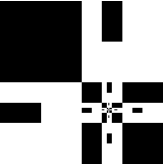
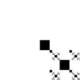
rule 33	rule 44	rule 50	rule 164
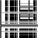
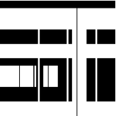
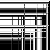
rule 14	rule 35	rule 168	rule 184

Figure 4: Matrices of some ECA with linear complexity. The first row shows matrices with striking fractal structure.

As an example we consider rule 132:

0 0 0 0

0 0 0 1

1 0 1 0

0 0 1 1

0 1 0 0

0 1 0 1

0 1 1 0

1 1 1 1

Figure 5 shows the fractal structure of its matrices. The space time diagram gives an explanation. Any block consisting of several 1’s, shrinks at every time step by 1 at each end, and either vanishes or remains a single 1, depending on the parity of its length.

         

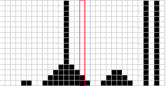
Figure 5: A space time diagram for rule 132 (left) and one matrix of its families (right). Note that in this matrix the lower right quadrant has the same structure as the matrix itself.

Lemma 10.

For rule 132 we have ${d_{n}=n+1}$.

Proof.

For an upper bound we give a very simple communication protocol. If the center is $0$, no communication at all is needed, as the answer will always be $0$. Now suppose the center is $1$. It is part of a block consisting of $k$ cells on Alice’s side, and of $l$ cells on Bob’s side, where $0\leq k,l\leq n$. Now Alice sends $k$ to Bob, and Bob answers $1$ if $k=l$ and $0$ otherwise. The protocol is correct, since after $n$ steps the center will remain $1$ only if it is in the center of an even length block or if it is distant by at least $n$ to each end of the block. For the protocol, Alice needs to send a number out of $n+1$ different values. It would be the same if Bob starts first. Therefore $d_{n}\leq n+1$.

For the lower bound, we give a submatrix in $M_{0}^{n}$ which is the identity. This submatrix is of dimension $(n+1)\times(n+1)$, which will show that there are at least $n+1$ different rows and at least as must different columns. Let $R_{k}$ be the row in $M_{0}^{n}$ corresponding to $0^{n-k}1^{k}$, and let $C_{l}$ be the column corresponding to $1^{l}0^{n-l}$. The submatrix made up of the intersection of rows $R_{k}$ and columns $C_{l}$ for $0\leq k,l\leq n$ is the identity matrix. ∎

This example is also interesting because the number of different rows in $M_{c}^{n}$ is $1$ if $c=0$ and $n+1$ if $c=1$, while for most rules the number of different rows seems to be the same (or at least similar) for the two families of matrices.

         

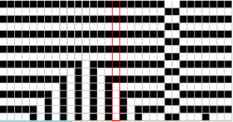
Figure 6: A space time diagram for rule 23 (left) and one matrix of its families (right). Note that there is a square in the matrix, smaller by 1/4 in height and width which has the same structure as the matrix itself.

Another example is rule 23:

1 0 0 0

1 0 0 1

1 0 1 0

0 0 1 1

1 1 0 0

0 1 0 1

0 1 1 0

0 1 1 1

In this rule, cells become alternatively 0 and 1 with exception of those being inside a block of alternating 0’s and 1’s. Since the neighboring cells of such a block alternate their states, a block shrinks at both ends by 2 cells every second time steps. One can apply the same method to prove $d_{n}=n+1$.

7 ECA with other complexity

The ECA of this class are not well understood yet. For example, it contains rules 110 and 54, which are conjectured to be computation universal. However for larger cell states we were able to prove polynomial and even exponential complexity for some CA.

The following CA with $3$ states has quadratic complexity and the construction can be generalized for more states to achieve complexity $\Theta(n^{k})$ for any $k$.

Let be the state set ${\{0,1,2\}}$. The cellular automata is defined for all $i,j,k$ by

$$f(i,j,k)=\left\{\begin{array}[]{ll}j&\text{if }j=0\text{ and }i=k,\\ \max\{i,j,k\}&\text{otherwise}.\end{array}\right.$$

Note that each state is quiescent. The global behavior can be explained like this (see figure 7). Every cell different from $0$ tends to expand in both directions. Whenever a $1$-expansion and a $2$-expansion meet, the $2$-expansion overrules the former. There is a single situation where a $0$ cell can remain $0$, it is when two expansions of the same state reach at the same time the left and right neighbor.

         

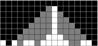
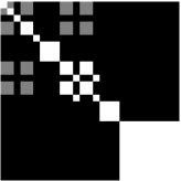
Figure 7: A space time diagram for the 3-state CA, where 0=white, 1=gray, 2=black (left) and one matrix $M_{0}^{n}$ of its families (right).

To make this statement formal, consider the cell at position $0$. Let $r_{2}$ be the position of the first state-2-cell on the right between $1$ and $n$, and $\infty$ if there is no such cell. Let $r_{1}$ be the position of the first state-1-cell between $1$ and $r_{2}-1$ and $\infty$ if there is no such cell. The positions $l_{1},l_{2}$ are defined in the same manner for the left neighborhood. Now we can completely determine the cell state after $n$ steps.

• If the cell was in state $2$, then it remains $2$ forever.

• If the cell was in state $1$, then it remains $1$ after $n$ steps if and only if $l_{2}<-n$ and $n<r_{2}$.

• If the cell was in state $0$, then it remains $0$ after $n$ steps if and only if ($l_{2}<-n$ and $n<r_{2}$ or $-l_{2}=r_{2}$) and ($l_{1}<-n$ and $n<r_{1}$ or $-l_{1}=r_{1}$).

From these observations we can determine its complexity.

Lemma 11.

The complexity of the CA defined above is $d_{n}\in\Theta(n^{2})$.

Proof.

We will construct $\Omega(n^{2})$ different rows in the matrix $M_{0}^{n}$, which will suffice for the lower bound by symmetry of the matrix. For every $0\leq j\leq i\leq n$ let be $R_{i,j}$ the row corresponding to the left neighborhood

$$\underbrace{2\cdots 2}_{n-i}\underbrace{1\cdots 1}_{i-j}\underbrace{0\cdots 0}_{j}.$$

Let be $C_{i,j}$ the column corresponding to the similar (reversed) right neighborhood. Then row $R_{i,j}$ is $0$ only at column $C_{i,j}$, showing that all rows $R_{i,j}$ are different.

Conversely for the upper bound, it is clear from the above description of the rule that a correct one-way communication protocol can be achieved with complexity ${2\lceil\log_{2}(n+1)\rceil}$, since Alice needs only to send the numbers $l_{1},l_{2}$ to Bob, while each can have only $n+1$ different values. ∎

We show now a very well known and simple CA, which has exponential complexity.

Let be state set $\{0,1,\tilde{0},\tilde{1}\}$. We define the cellular automata $f$ such that $f^{n}(u,1,v)$ compares the strings $u$ and $v$, with $u\in\{0,1\}$ and $v\in\{\tilde{0},\tilde{1}\}$. Let be $x,c,y\in\{0,1\}$ and $z\in\{0,1,\tilde{0},\tilde{1}\}$, then

$$f(z,\tilde{c},\tilde{y})=\tilde{y}$$ (shift left to the center)

$$f(x,c,y)=x$$ (shift right to the center)

$$f(x,1,\tilde{y})=\left\{\begin{array}[]{ll}1&\text{if }x=y\\ 0&\text{if }x\neq y\end{array}\right.$$ (a difference makes the center 0)

For all other values $f$ is $0$.

Lemma 12.

The complexity $d_{n}$ of the CA defined above is exponential in $n$.

Proof.

Clearly $M_{1}^{n}$ contains at least $2^{n}$ different rows (among $4^{n}$): for every row indexed by ${u\in\{0,1\}^{n}}$ there is a single entry $1$, at a column $v$, where $v$ is the reverse dual of $u$, and any other row contains only $0$. ∎

8 Future directions

The purpose of this paper was to show a relationship between cellular automata and communication complexity. For this we deliberately made simple choices: elementary cellular automata and particular one-way communication. Our approach can be generalized in several ways:

• We partitioned evenly the $2n+1$ cells between Alice and Bob, and also fixed the center cell. This does not take into account asymmetric behavior for some CA. When $f^{n}$ is fixed, we can define a matrix representation $M_{p}^{n}$ of dimension $2^{p}\times 2^{2n+1-p}$ (for ${1\leq p\leq 2n+1}$) such that $M_{p}^{n}(u,v)=f(u\stackrel{{\scriptstyle\leftarrow}}{{v}})$, i.e. where Alice knows the $p$ leftmost cells and Bob the $n-p$ rightmost. Then an interesting complexity measure is:

  $$R_{n}=\max_{p}|rows(M_{p}^{n})|,$$

  where $|rows(\cdot)|$ stands for the number of different rows. The value of $p$ where the maximum is reached is non trivial and, while clearly connected to the global behavior, hard to predict from the local rule. A striking example is ECA rule 7 which has a bounded $d_{n}$ complexity due to its half-limited sensibility but has a linear $R_{n}$ complexity, maximum being reached around ${p=\frac{n}{3}}$, as indicated by brute force computations.

  Following this idea, we could as well define $R_{n}$ symmetrically on rows and columns as follows:

  $$R_{n}=\max_{p}\max\left\{|rows(M_{p}^{n})|,|cols(M_{p}^{n})|\right\}.$$

• The link between communication complexity and matrix representations is not reduced to Fact 3. Actually, many round communication complexity is lower-bounded by the log of the rank of the matrix representation (see [KN97]). Moreover, it is conjectured that a poly-log of the rank is also an upper-bound.

• Finally, considering the more general framework of all one-dimensional CA (with any radius and any state set), it is interesting to note that a classification based on the asymptotic behavior of $d_{n}$ has some very reassuring properties such as:

  • the class of a CA $A$ is “higher” than the class of any of its sub-CA ;

  • the complexity of the Cartesian product $A\times B$ is the product of the complexities of $A$ and $B$.

Another important issue of course, is to give mathematical rigorous proofs for the complexity of some ECA, which however is at least as difficult as understanding completely the global behavior.

9 Acknowledgment

We would like to thank Nicolas Ollinger for helpful discussions.

References

- [DM99] M. Delorme and J. Mazoyer, editors. Cellular Automata. Kluwer Academic Publishers, 1999.
- [Kar92] J. Kari. The nilpotency problem of one-dimensional cellular automata. SIAM J. on Computing, 21:571–586, 1992.
- [KN97] E. Kushilevitz and N. Nisan. Communication Complexity. Cambridge, 1997.
- [vN67] J. von Neumann. The theory of self reproducting cellular automata. University of Illinois Press, Urbana, Illinois, 1967.
- [Yao79] A.C. Yao. Some complexity questions related to distributed computing. In Proc. of 11th ACM Symposium on Theory of Computing, pages 209–213, 1979.