On the Reflexivity of Point Sets

Abstract

We introduce a new measure for planar point sets $S$ that captures a combinatorial distance that $S$ is from being a convex set: The reflexivity $\rho(S)$ of $S$ is given by the smallest number of reflex vertices in a simple polygonalization of $S$. We prove various combinatorial bounds and provide efficient algorithms to compute reflexivity, both exactly (in special cases) and approximately (in general). Our study considers also some closely related quantities, such as the convex cover number $\kappa_{c}(S)$ of a planar point set, which is the smallest number of convex chains that cover $S$, and the convex partition number $\kappa_{p}(S)$, which is given by the smallest number of convex chains with pairwise-disjoint convex hulls that cover $S$. We have proved that it is NP-complete to determine the convex cover or the convex partition number and have given logarithmic-approximation algorithms for determining each.

1 Introduction

In this paper, we study a fundamental combinatorial property of a discrete set, $S$, of points in the plane: What is the minimum number, $\rho(S)$, of reflex vertices among all of the simple polygonalizations of $S$? A polygonalization of $S$ is a closed tour on $S$ whose straight-line embedding in the plane defines a connected cycle without crossings, i.e., a simple polygon. A vertex of a simple polygon is reflex if it has interior angle greater than $\pi$. We refer to $\rho(S)$ as the reflexivity of $S$. We let $\rho(n)$ denote the maximum possible value of $\rho(S)$ for a set $S$ of $n$ points.

In general, there are many different polygonalizations of a point set $S$. There is always at least one: simply connect the points in angular order about some point interior to the convex hull of $S$ (e.g., the center of mass suffices). A set $S$ has precisely one polygonalization if and only if it is in convex position; in general, though, a point set has numerous polygonalizations. Studying the set of polygonalizations (e.g., counting them, enumerating them, or generating a random element) is a challenging and active area of investigation in computational geometry [5, 6, 9, 18, 20, 39].

The reflexivity $\rho(S)$ quantifies, in a combinatorial sense, the degree to which the set of points $S$ is in convex position. See Figure 1 for an example. We remark that there are other notions of combinatorial “distance” from convexity of a point set $S$, e.g., the minimum number of points to delete from $S$ in order that the remaining point set is in convex position, the number of convex layers, or the minimum number of changes in the orientation of triples of points of $S$ in order to transform $S$ into convex position.

Figure 1: Two polygonalizations of a point set, one (left) using 7 reflex vertices and one (right) using only 3 reflex vertices.

We have conducted a formal study of reflexivity, both in terms of its combinatorial properties and in terms of an algorithmic analysis of the complexity of computing it, exactly or approximately. Some of our attention is focussed on the closely related convex cover number of $S$, which gives the minimum number of convex chains (subsets of $S$ in convex position) that are required to cover all points of $S$. For this question, we distinguish between two cases: The convex cover number, $\kappa_{c}(S)$, is the smallest number of convex chains required to cover $S$; the convex partition number, $\kappa_{p}(S)$, is the smallest number of convex chains with pairwise-disjoint convex hulls required to cover $S$. Note that nested chains are feasible for a convex cover but not for a convex partition.

Motivation.

In addition to the fundamental nature of the questions and problems we address, we are also motivated to study reflexivity for several other reasons:

(1) An application motivating our original investigation is that of meshes of low stabbing number and their use in performing ray shooting efficiently. If a point set $S$ has low reflexivity or a low convex partition number, then it has a triangulation of low stabbing number, which may be much lower than the general $O(\sqrt{n})$ upper bound guaranteed to exist ([1, 22, 38]). For example, if the reflexivity is $O(1)$, then $S$ has a triangulation with stabbing number $O(\log n)$.

(2) Classifying point sets by their reflexivity may give us some structure for dealing with the famously difficult question of counting and exploring the set of all polygonalizations of $S$. See [20, 39] for some references to this problem.

(3) There are several applications in computational geometry in which the number of reflex vertices of a polygon can play an important role in the complexity of algorithms. If one or more polygons are given to us, there are many problems for which more efficient algorithms can be written with complexity in terms of “$r$” (the number of reflex vertices), instead of “$n$” (the total number of vertices), taking advantage of the possibility that we may have $r\ll n$ for some practical instances (see, e.g., [23, 27]). The number of reflex vertices also plays an important role in convex decomposition problems for polygons; see Keil [28] for a recent survey, and see Agarwal, Flato, and Halperin [2] for applications of convex decompositions to computing Minkowski sums of polygons.

(4) Reflexivity is intimately related to the issue of convex cover numbers, which has roots in the classical work of Erdős and Szekeres [16, 17], and has been studied more recently by Urabe et al. [25, 26, 35, 36].

(5) Our problems are related to some problems in curve (surface) reconstruction, where the goal is to obtain a “good” polygonalization of a set of sample points (see, e.g., [8, 12, 13]).

Related Work.

The study of convex chains in finite planar point sets is the topic of classical papers by Erdős and Szekeres [16, 17], who showed that any point set of size $n$ has a convex subset of size $t=\Omega(\log n)$. This is closely related to the convex cover number $\kappa_{c}$, since it implies an asymptotically tight bound on $\kappa_{c}(n)$, the worst-case value for sets of size $n$. There are still a number of open problems related to the exact relationship between $t$ and $n$; see, for example, [33] for recent developments.

Other issues have been considered, such as the existence and computation ([14]) of large “empty” convex subsets (i.e., with no points of $S$ interior to their hull); this is related to the convex partition number, $\kappa_{p}(S)$. It was shown by Horton [24] that there are sets with no empty convex chain larger than 6; this implies that $\kappa_{p}(n)\geq n/6$.

Tighter worst-case bounds on $\kappa_{p}(n)$ were given by Urabe [35, 36], who shows that $\lceil(n-1)/4\rceil\leq\kappa_{p}(n)\leq\lceil 2n/7\rceil$ and that $\kappa_{c}(n)=\Theta(n/\log n)$ (with the upper and lower bounds having a gap of roughly a factor of 2). (Urabe [37] also studies the convex partitioning problem in $\Re^{3}$, where, in particular, the upper bound on $\kappa_{p}(n)$ is shown to be $\lceil 2n/9\rceil$.) Most recently, Hosono and Urabe [26] have obtained improved bounds on the size of a partition of a set of points into disjoint convex quadrilaterals, which has the consequence of improving the upper bound on $\kappa_{p}(n)$: $\kappa_{p}(n)\leq\lceil 5n/18\rceil$ and $\kappa_{p}(n)\leq(3n+1)/11$ for $n=11\cdot 2^{k-1}-4$ ($k\geq 1$). The remaining gaps in the constants between upper and lower bounds for $\kappa_{c}(n)$ and $\kappa_{p}(n)$ (as well as the gap that our bounds exhibit for reflexivity in terms of $n$) all point to the apparently common difficulty of these combinatorial problems on convexity.

For a given set of points, we are interested in polygonalizations of the points that are “as convex as possible”. This has been studied in the context of TSP (traveling salesperson problem) tours of a point set $S$, where convexity of $S$ implies (trivially) the optimality of a convex tour. Convexity of a tour can be characterized by two conditions. If we drop the global condition (i.e., no crossing edges), but keep the local condition (i.e., no reflex vertices), we get “pseudo-convex” tours. In [19] it was shown that any set with $|S|\geq 5$ has such a pseudo-convex tour. It is natural to require the global condition of simplicity instead, and minimize the number of local violations – i.e., the number of reflex vertices. This kind of problem is similar to that of minimizing the total amount of turning in a tour, as studied by Aggarwal et al. [4].

The number of polygonalizations on $n$ points is, in general, exponential in $n$; García et al. [20] prove a lower bound of $\Omega(4.64^{n})$.

Another related problem is studied by Hosono et al. [25]: Compute a polygonalization $P$ of a point set $S$ such that the interior of $P$ can be decomposed into a minimum number ($f(S)$) of empty convex polygons. They prove that $\lfloor(n-1)/4\rfloor\leq f(n)\leq\lfloor(3n-2)/5\rfloor,$ where $f(n)$ is the maximum possible value of $f(S)$ for sets $S$ of $n$ points. The authors conjecture that $f(n)$ grows like $n/2$. For reflexivity $\rho(n)$, we show that ${\lfloor n/4\rfloor}\leq\rho(n)\leq{\lceil n/2\rceil}$ and conjecture that $\rho(n)$ grows like $n/4$, which, if true, would imply that $f(n)$ grows like $n/2$.

We mention one final related problem. A convex decomposition of a point set $S$ is a convex planar polygonal subdivision of the convex hull of $S$ whose vertices are $S$. Let $g(S)$ denote the minimum number of faces in a convex decomposition of $S$, and let $g(n)$ denote the maximum value of $g(S)$ over all $n$-point sets $S$. It has been conjectured ([34]) that $g(n)=n+c$ for some constant $c$, and it is known that $g(n)\leq 3n/2$ ([34]) and that $n+2\leq g(n)$ ([7]).

Summary of Main Results.

We have both combinatorial and algorithmic results on reflexivity. Our combinatorial results include

• Tight bounds on the worst-case value of $\rho(S)$ in terms of $n_{I}$, the number of points of $S$ interior to the convex hull of $S$; in particular, we show that $\rho(S)\leq{\lceil n_{I}/2\rceil}$ and that this upper bound can be achieved by a class of examples.

• Upper and lower bounds on $\rho(S)$ in terms of $n=|S|$; in particular, we show that ${\lfloor n/4\rfloor}\leq\rho(n)\leq{\lceil n/2\rceil}$. In the case in which $S$ has two layers, we show that $\rho(S)\leq{\lceil n/4\rceil}$, and this bound is tight.

• Upper and lower bounds on “Steiner reflexivity”, which is defined with respect to the class of polygonalizations that allow Steiner vertices (not from the input set $S$).

Our algorithmic results include

• We prove that it is NP-complete to compute the convex cover number ($\kappa_{c}(S)$) or the convex partition number ($\kappa_{p}(S)$), for a given point set $S$.

• We give polynomial-time approximation algorithms, having approximation factor $O(\log n)$, for the problems of computing convex cover number, convex partition number, or Steiner reflexivity of $S$.

• We give efficient exact algorithms to test if $\rho(S)=1$ or $\rho(S)=2$.

In Section 6 we study a closely related problem – that of determining the “inflectionality” of $S$, defined to be the minimum number of inflection edges (joining a convex to a reflex vertex) in any polygonalization of $S$. We give an $O(n\log n)$ time algorithm to determine an inflectionality-minimizing polygonalization, which we show will never need more than 2 inflection edges.

2 Preliminaries

Throughout this paper, $S$ will be a set of $n$ points in the plane $\Re^{2}$. A polygonalization, $P$, of $S$ is a simple polygon whose vertex set is $S$. Let ${\cal P}$ be the set of all polygonalizations of $S$. Note that ${\cal P}$ is not empty, since any point set $S$ having $n\geq 3$ points has at least one polygonalization (e.g., the star-shaped polygonalization obtained by sorting points of $S$ angularly about a point interior to the convex hull of $S$).

Each vertex of a simple polygon $P$ is either reflex or convex, according to whether the interior angle at the vertex is greater than $\pi$ or less than or equal to $\pi$, respectively. We let $r(P)$ (resp., $c(P)$) denote the number of reflex (resp., convex) vertices of $P$. We define the reflexivity of a planar point set $S$ to be $\rho(S)=\min_{P\in{\cal P}}r(P)$. Similarly, the convexivity of a planar point set $S$ is defined to be $\chi(S)=\max_{P\in{\cal P}}c(P)$. Note that $\chi(S)=n-\rho(S)$. We let $\rho(n)=\max_{|S|=n}\rho(S)$.

We let $\textrm{CH}(S)$ denote the convex hull of $S$. The point set $S$ is partitioned into (convex) layers, $S_{1},S_{2},\ldots$, where the first layer is given by the set $S_{1}$ of points of $S$ on the boundary of $\textrm{CH}(S)$, and the $i$th layer, $S_{i}$ ($i\geq 2$) is given by the set of points of $S$ on the boundary of $\textrm{CH}(S\setminus(S_{1}\cup\cdots\cup S_{i-1}))$. We say that $S$ has $k$ layers or onion depth $k$ if $S_{k}\neq\emptyset$, while $S_{k+1}=\emptyset$. We say that $S$ is in convex position (or forms a convex chain) if it has one layer (i.e., $S=S_{1}$).

A Steiner point is a point not in the set $S$ that may be added to $S$ in order to improve some structure of $S$. We define the Steiner reflexivity $\rho^{\prime}(S)$ to be the minimum number of reflex vertices of any simple polygon with vertex set $V\supset S$. We let $\rho^{\prime}(n)=\max_{|S|=n}\rho^{\prime}(S)$. The Steiner convexivity, $\chi^{\prime}(S)$, is defined similarly. A convex cover of $S$ is a set of subsets of $S$ whose union covers $S$, such that each subset is a convex chain (a set in convex position). A convex partition of $S$ is a partition of $S$ into subsets each of which is in convex position, such that the convex hulls of the subsets are pairwise disjoint. We define the convex cover number, $\kappa_{c}(S)$, to be the minimum number of subsets in a convex cover of $S$. We similarly define the convex partition number, $\kappa_{p}(S)$. We denote by $\kappa_{c}(n)$ and $\kappa_{p}(n)$ the worst-case values for sets of size $n$.

Finally, we state a basic property of polygonalizations of point sets.

Lemma 2.1.

In any polygonalization of $S$, the points of $S$ that are vertices of the convex hull of $S$ are convex vertices of the polygonalization, and they occur in the polygonalization in the same order in which they occur along the convex hull.

Proof.

Any polygonalization $P$ of $S$ must lie within the convex hull of $S$, since edges of the polygonalization are convex combinations of points of $S$. Thus, if $p\in S$ is a vertex of $\textrm{CH}(S)$, then the local neighborhood of $P$ at $p$ lies within a convex cone, so $p$ must be a convex vertex of $P$.

Consider a clockwise traversal of $P$ and let $p$ and $q$ be two vertices of $\textrm{CH}(S)$ occurring consecutively along $P$. Then $p$ and $q$ must also appear consecutively along a clockwise traversal of the boundary of $\textrm{CH}(S)$, since the subchain of $P$ linking $p$ to $q$ partitions $\textrm{CH}(S)$ into a region to its left (which is outside the polygon $P$) and a region to its right (which must contain all points of $S$ not in the subchain). ∎

3 Combinatorial Bounds

In this section we establish several combinatorial results on reflexivity and convex cover numbers.

3.1 Reflexivity

One of our main combinatorial results establishes an upper bound on the reflexivity of $S$ that is worst-case tight in terms of the number $n_{I}$ of points interior to the convex hull, $\textrm{CH}(S)$, of $S$. Since, by Lemma 2.1, the points of $S$ that are vertices of $\textrm{CH}(S)$ are required to be convex vertices in any (non-Steiner) polygonalization of $S$, the bound in terms of $n_{I}$ seems to be quite natural.

Theorem 3.1.

Let $S$ be a set of $n$ points in the plane, $n_{I}$ of which are interior to the convex hull $\textrm{CH}(S)$. Then $\rho(S)\leq{\lceil n_{I}/2\rceil}$.

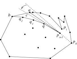
Figure 2: Computing a polygonalization with at most ${\lceil n_{I}/2\rceil}$ reflex vertices.

Proof.

We describe a polygonalization in which at most half of the interior points are reflex. We begin with the polygonalization of the convex hull vertices that is given by the convex polygon bounding the hull. We then iteratively incorporate interior points of $S$ into the polygonalization. Fix a point $p_{0}$ that lies on the convex hull of $S$. At a generic step of the algorithm, the following invariants hold: (1) our polygonalization consists of a simple polygon, $P$, whose vertices form a subset of $S$; and (2) all points $S^{\prime}\subset S$ that are not vertices of $P$ lie interior to $P$; in fact, the points $S^{\prime}$ all lie within the subpolygon, $Q$, to the left of the diagonal $p_{0}p_{i}$, where $p_{i}$ is a vertex of $P$ such that the subchain of $\partial P$ from $p_{i}$ to $p_{0}$ (counter-clockwise) together with the diagonal $p_{0}p_{i}$ forms a convex polygon ($Q$). If $S^{\prime}$ is empty, then $P$ is a polygonalization of $S$ and we are done; thus, assume that $S^{\prime}\neq\emptyset$. Define $p_{i+1}$ to be the first point of $S^{\prime}$ that is encountered when sweeping the ray ${\overrightarrow{p_{0}p_{i}}}$ counter-clockwise about its endpoint $p_{0}$. Then we sweep the subray with endpoint $p_{i+1}$ further counter-clockwise, about $p_{i+1}$, until we encounter another point, $q$, of $S^{\prime}$. (If $|S^{\prime}|=1$, we can readily incorporate $p_{i+1}$ into the polygonalization, increasing the number of reflex vertices by one.) Now the ray ${\overrightarrow{p_{i+1}q}}$ intersects the boundary of $P$ at some point $c\in ab$ on the boundary of $Q$.

As a next step, we modify $P$ to include interior points $p_{i+1}$ and $q$ (and possibly others as well) by replacing the edge $ab$ with the chain $(a,p_{i+1}$, $q$, $q_{1},\ldots$, $q_{k},b)$, where the points $q_{i}$ are interior points that occur along the chain we obtain by “pulling taut” the chain $(q,c,b)$. In this “gift wrapping” fashion, we continue to rotate rays counter-clockwise about each interior point $q_{i}$ that is hit until we encounter $b$. This results in incorporating at least two new interior points (of $S^{\prime}$) into the polygonalization $P$, while creating only one new reflex vertex (at $p_{i+1}$). It is easy to check that the invariants (1) and (2) hold after this step. ∎

In fact, the upper bound of Theorem 3.1, $\rho(S)\leq{\lceil n_{I}/2\rceil}$, is tight in the worst case, as we now argue based on the special configuration of points, $S=S_{0}(n)$, in Figure 3. The set $S_{0}(n)$ is defined for any integer $n\geq 6$, as follows: ${\lceil n/2\rceil}$ points are placed in convex position (e.g., forming a regular ${\lceil n/2\rceil}$-gon), forming the convex hull $\textrm{CH}(S)$, and the remaining $n_{I}={\lfloor n/2\rfloor}$ interior points are also placed in convex position, each one placed “just inside” $\textrm{CH}(S)$, near the midpoint of an edge of $\textrm{CH}(S)$. The resulting configuration $S_{0}(n)$ has two layers in its convex hull.

Figure 3: Left: The configuration of points, $S_{0}(n)$, which has reflexivity $\rho(S_{0}(n))\geq{\lceil n_{I}/2\rceil}$. Right: A polygonalization having ${\lceil n_{I}/2\rceil}$ reflex vertices.

Lemma 3.2.

For any $n\geq 6$, $\rho(S_{0}(n))\geq{\lceil n_{I}/2\rceil}\geq{\lfloor n/4\rfloor}$.

Proof.

Let $(x_{1},x_{2},\ldots,x_{{\lceil n/2\rceil}})$ denote the points of $S_{0}(n)$ on the convex hull, in clockwise order, and let $(v_{1},v_{2},\ldots,v_{{\lfloor n/2\rfloor}})$ denote the remaining points of $S_{0}(n)$, with $v_{i}$ just inside the convex hull edge $(x_{i},x_{i+1})$. We define $x_{{\lceil n/2\rceil}+1}=x_{1}$.

Consider any polygonalization, $P$, of $S_{0}(n)$. From Lemma 2.1 we know that the points $x_{i}$ are convex vertices of $P$, occurring in the order $x_{1}$, $x_{2},\ldots$, $x_{{\lceil n/2\rceil}}$ around the boundary of $P$. Consider the subchain, $\gamma_{i}$, of $\partial P$ that goes from $x_{i}$ to $x_{i+1}$, clockwise around $\partial P$. Let $m_{i}$ denote the number of points $v_{j}$, interior to the convex hull of $S_{0}(n)$, that appear along $\gamma_{i}$.

If $m_{i}=0$, $\gamma_{i}=x_{i}x_{i+1}$. If $m_{i}=1$, then $\gamma_{i}=x_{i}v_{i}x_{i+1}$ and $v_{i}$ is a reflex vertex of $P$; to see this, note that $v_{i}$ lies interior to the triangle determined by $x_{i}$, $x_{i+1}$, and any $v_{j}$ with $j\neq i$. If $m_{i}>1$, then we claim that (a) $v_{i}$ must be a vertex of the chain $\gamma_{i}$, (b) $v_{i}$ is a convex vertex of $P$, and (c) any other point $v_{j}$, $j\neq i$, that is a vertex of $\gamma_{i}$ must be a reflex vertex of $P$. This claim follows from the fact that the points $x_{i}$, $x_{i+1}$, and any nonempty subset of $\{v_{j}:j\neq i\}$ are in convex position, with the point $v_{i}$ interior to the convex hull. Refer to Figure 4, where the subchain $\gamma_{i}$ is shown dashed.

Figure 4: Proof of the lower bound: $\rho(S_{0}(n))\geq{\lceil n_{I}/2\rceil}\geq{\lfloor n/4\rfloor}$.

Thus, the number of reflex vertices of $P$ occurring along $\gamma_{i}$ is in any case at least ${\lceil m_{i}/2\rceil}$, and we have

$$\rho(S_{0}(n)) \geq \sum{\lceil m_{i}/2\rceil}$$

$$\geq \left\lceil\sum(m_{i}/2)\right\rceil={\lceil n_{I}/2\rceil}\geq{\lfloor n/4\rfloor}.$$

∎

Since $n_{I}\leq n$, the corollary below is immediate from Theorem 3.1 and Lemma 3.2. The gap in the bounds for $\rho(n)$, between ${\lfloor n/4\rfloor}$ and ${\lceil n/2\rceil}$, remains an intriguing open problem. While our combinatorial bounds are worst-case tight in terms of $n_{I}$ (the number of points of $S$ whose convexity/reflexivity is not forced by the convex hull of $S$), they are not worst-case tight in terms of $n$.

Corollary 3.3.

${\lfloor n/4\rfloor}\leq\rho(n)\leq{\lceil n/2\rceil}$.

Based on experience with a software tool developed by A. Dumitrescu that computes, in exponential time, the reflexivity of user-specified or randomly generated point sets, as well as the proven behavior of $\rho(n)$ for small values of $n$ (see Section 3.5), we make the following conjecture:

Conjecture 3.4.

$\rho(n)={\lfloor n/4\rfloor}$.

3.2 Steiner Points

If we allow Steiner points in the polygonalizations of $S$, the reflexivity of $S$ may go down substantially, as the example in Figure 5 shows. In fact, the illustrated class of examples shows that the use of Steiner points may allow the reflexivity to go down by a factor of two. The Steiner reflexivity, $\rho^{\prime}(S)$, of $S$ is the minimum number of reflex vertices of any simple polygon with vertex set $V\supset S$. We conjecture that $\rho^{\prime}(S)\geq\rho(S)/2$ for any set $S$, which would imply that this class of examples (essentially) maximizes the ratio $\rho(S)/\rho^{\prime}(S)$.

Conjecture 3.5.

For any set $S$ of points in the plane, $\rho^{\prime}(S)\geq\rho(S)/2$.

Figure 5: Left: A point set $S$ having reflexivity $\rho(S)=r$. Right: The reflexivity of $S$ when Steiner points are permitted is substantially reduced from the no-Steiner case: $\rho^{\prime}(S)=r/2$.

We have seen (Corollary 3.3) that ${\lfloor n/4\rfloor}\leq\rho(n)\leq{\lceil n/2\rceil}$. We now show that allowing Steiner points in the polygonalization allows us to prove a smaller upper bound, while still being able to prove roughly the same lower bound:

Theorem 3.6.

$$\left\lceil\frac{n-1}{4}\right\rceil-1\leq\rho^{\prime}(n)\leq\left\lceil\frac{n}{3}\right\rceil.$$

Proof.

For the upper bound, we give a specific method of constructing a polygonalization (with Steiner points) of a set $S$ of $n$ points. Sort the points $S$ by their $x$-coordinates and group them into consecutive triples. Let $p_{n+1}$ denote a (Steiner) point with a very large positive $y$-coordinate and let $p_{0}$ denote a (Steiner) point with a very negative $y$-coordinate. Each triple, together with either point $p_{n+1}$ or point $p_{0}$, forms a convex quadrilateral. Then, we can polygonalize $S$ using one reflex (Steiner) point per triple, as shown in Figure 6, placed very close to $p_{n+1}$ or $p_{0}$ accordingly. This polygonalization has at most ${\lceil n/3\rceil}$ reflex points.

For the lower bound, we consider the configuration of $n$ points, $S$, used in Urabe [35] to prove that $\kappa_{p}(n)\geq{\lceil(n-1)/4\rceil}$. For this set $S$ of $n$ points, let $P$ be a Steiner polygonalization having $r$ reflex vertices. Then the simple polygon $P$ can be partitioned into $r+1$ (pairwise-disjoint) convex pieces; this is a simple observation of Chazelle [10] (see Theorem 2.5.1 of [32]). The points $S$ occur as a subset of the vertices of these pieces; thus, the partitioning also decomposes $S$ into at most $r+1$ subsets, each in convex position. Since $\kappa_{p}(n)\geq\lceil(n-1)/4\rceil$, we get that $r\geq\lceil(n-1)/4\rceil-1$. ∎

Figure 6: Polygonalization of $n$ points using only ${\lceil n/3\rceil}$ reflex (Steiner) points.

3.3 Two-Layer Point Sets

Let $S$ be a point set that has two (convex) layers. It is clear from our repeated use of the example in Figure 3 that this is a natural case that is a likely candidate for worst-case behavior. With a very careful analysis of this case, we are able to obtain tight combinatorial bounds on the worst-case reflexivity in terms of $n$.

Theorem 3.7.

Let $S$ be a set of $n$ points having two layers. Then $\rho(S)\leq{\lceil n/4\rceil}$, and this bound is tight in the worst case.

Proof.

Consider a set $S$ of $n$ points with onion depth two. Let $h$ be the number of points on the convex hull. Thus there are $n-h$ points on the interior onion layer. Let the points on the convex hull be $a_{0},a_{1},\dots,a_{h-1}$ in clockwise order. Let the points on the interior onion layer be $b_{0},b_{1},\dots,b_{n-h-1}$ in clockwise order. All arithmetic involving the subscripts of the $a$’s and $b$’s is done mod $h$ and mod $(n-h)$, respectively.

Fact 3.8.

In any polygonalization of $S$ each pocket has at least one reflex vertex.

Proof.

This follows from the fact that the polygon defined by the pocket and its convex hull edge must have at least three convex vertices (as does any simple polygon). ∎

Consider any point $b_{i}$ on the interior onion layer. Let the intersection of ray ${\overrightarrow{b_{i-1}b_{i}}}$ with the convex hull be $x_{i}\in a_{j}a_{j+1}$. We call the directed segment $b_{i}x_{i}$ the spoke $s_{i}$ originating at $b_{i}$, and we say that the spoke $s_{i}$ belongs to the convex hull segment $a_{j}a_{j+1}$ and the segment $a_{j}a_{j+1}$ has the spoke $s_{i}$. Refer to Figure 7.

The number of spokes a convex hull segment has is called its spoke count. Let $c_{j}$ be the spoke count of convex hull segment $a_{j}a_{j+1}$. Clearly there are $n-h$ spokes $s_{0},s_{1},\dots,s_{n-h-1}$ and each spoke belongs to exactly one convex hull segment (assuming no degeneracy). Also for all $j$, $0\leq c_{j}\leq n-h$ and $\sum_{j=0}^{h-1}c_{j}=n-h$.

Figure 7: The situation for a point set with two layers.

Consider any convex hull edge $a_{j}a_{j+1}$ with non-zero spoke count $c_{j}$. Assume that the originating points of its spokes are $b_{i}$, $b_{i+1}$,$\dots$, $b_{i+c_{j}-1}$ in clockwise order. Then the pocket $a_{j}$, $b_{i}$, $b_{i+1}$,$\dots$, $b_{i+c_{j}-1}$, $a_{j+1}$ is called the standard pocket for the convex hull edge $a_{j}a_{j+1}$. See Figure 8.

Figure 8: Standard pockets.

Fact 3.9.

A standard pocket has exactly one reflex vertex.

Proof.

Vertices $b_{i+1},b_{i+2},\dots,b_{i+c_{j}-2}$ are convex, since the angles at these vertices are the interior angles of the inner onion layer. The vertex $b_{i+c_{j}-1}$ is convex because point $a_{j+1}$ is on the right of directed line $b_{i+c_{j}-2}b_{i+c_{j}-1}$. The vertex $b_{i}$ is reflex because there has to be at least one reflex vertex in any pocket. ∎

Fact 3.10.

No two standard pockets intersect each other, except possibly at their endpoints.

Proof.

The annulus between the two onion rings is divided into $n-h$ disjoint regions by the spokes. A standard pocket for segment $a_{j}a_{j+1}$ may share a region with each of the standard pockets (if any) for segments $a_{j-1}a_{j}$ and $a_{j}a_{j+1}$. In such shared regions two pockets have a segment each. The two segments do not intersect because the two segments are obtained by rotating two spokes about their points of origin until their intersection with the convex hull reaches a vertex. The two segments can hence either remain disjoint or share an endpoint. ∎

We obtain the standard polygonalization by connecting all standard pockets, in order, using convex hull segments with zero spoke count. See Figure 8.

Fact 3.11.

The number of reflex vertices in the standard polygonalization is at most ${\lfloor n/2\rfloor}$.

Proof.

The number of standard pockets can neither exceed the number of convex hull segments $h$ nor the number of internal points, $n-h$. Hence, this polygonalization has at most $\min\{h,n-h\}$ standard pockets and hence reflex vertices. This can be at most ${\lfloor n/2\rfloor}$. ∎

Consider a convex hull segment $a_{j}a_{j+1}$ that has a non-zero spoke count $c_{j}$. Assume that the origins of its spokes are $b_{i},b_{i+1},\dots,b_{i+c_{j}-1}$. We call the pocket $a_{j}$, $b_{i-i}$, $b_{i}$, $b_{i+1},\dots$, $b_{i+c_{j}-1}$, $a_{j+1}$ the premium pocket for convex hull segment $a_{j}a_{j+1}$. Note that the premium pocket of a segment has one more point than its standard pocket. We obtain the premium polygonalization as follows: Start with the convex hull. Process convex hull segments in clockwise order beginning anywhere. If the convex hull segment $a_{i}a_{i+1}$ has spoke count greater than or equal to two, replace the edge with its standard pocket. If the spoke count is zero, do nothing. If the spoke count is one, move to the next segment with non-zero spoke count and replace it with its premium pocket provided that it is not already processed. If the next segment with non-zero spoke count was already processed, replace the segment being processed with its standard pocket, and we are done. One can verify that this process gives a valid polygonalization.

Fact 3.12.

The number of reflex vertices in a premium polygonalization is at most ${\lfloor n/3\rfloor}$.

Proof.

In the premium polygonalization, each pocket has at least one reflex and one convex vertex, with the exception of the last pocket created, which may have only a single reflex vertex. Thus, the number of pockets created cannot exceed ${\lfloor(n-h+1)/2\rfloor}$. Also, the number of pockets cannot exceed the number of convex hull edges, $h$. Thus, the number of pockets and, therefore, the number of reflex vertices cannot exceed $\min\{h,{\lfloor(n-h+1)/2\rfloor}\}$, which can be at most ${\lfloor n/3\rfloor}$. ∎

We now define the intruding polygonalization, as follows: Start with the convex hull. Process convex hull segments in clockwise order, beginning anywhere. We consider cases, depending on the spoke count, $c_{j}$, of the convex hull segment $a_{j}a_{j+1}$:

$c_{j}=0$

Do nothing.

$c_{j}\geq 3$

Replace $a_{j}a_{j+1}$ with a standard pocket.

$c_{j}=1$

Replace the next non-zero count unprocessed hull segment with its premium pocket. (If no such non-zero count unprocessed segment exists, then replace $a_{j}a_{j+1}$ by its standard pocket and stop.)

$c_{j}=2$

We distinguish two subcases:

Case A

If this is the last segment to be processed or if the sequence of spoke counts following this segment begins with either 0, or a count $\geq 4$, or an odd number of 1’s, or an even number of 1’s followed by a zero, do the following: Replace $a_{j}a_{j+1}$ with its standard pocket.

Case B

If there are an even number of 1’s followed by a non-zero spoke count, or if the sequence begins with 2 or 3, do one of the following, depending on the current “mode”; initially, the mode is “normal.”

Normal Mode. Replace $a_{j+1}a_{j+2}$ with its premium pocket. This leaves one of the originating points of $a_{j}a_{j+1}$; call a point $P$ of this type the pending point. Go into “Point Pending Mode.”

Point Pending Mode. Let the origins of the spokes of $a_{j}a_{j+1}$ be $b_{i},\dots,b_{i+c_{j}-1}$. Find the first point of intersection of the ray ${\overrightarrow{Pb_{i}}}$ with the current polygonalization. There are only two choices for where the point of intersection can lie.

If the point of intersection lies on $a_{j}a_{j+1}$, treat ray ${\overrightarrow{Pb_{i}}}$ as a spoke of $a_{j}a_{j+1}$, thus increasing $c_{j}$ by 1. Now replace $a_{j}a_{j+1}$ by its standard pocket, and return to the “Normal Mode.”

If the point of intersection lies on $a_{j}b_{i-1}$, replace $a_{j}b_{i-1}$ with $a_{j}b_{i}Pb_{i-1}$. This reduces $c_{j}$ from 2 to 1. Now handle as in Case 1.

Fact 3.13.

The intruding polygonalization produces a valid (non-crossing) polygonalization of $S$, with at most ${\lfloor n/4\rfloor}$ reflex vertices.

Proof.

It is straightforward to check each case to make certain that the polygonalization is valid. We prove the bound on the number of reflex vertices by charging each reflex vertex created to a set of 4 input points.

In case $c_{j}=0$, we do not create any reflex points.

In case $c_{j}\geq 3$, we create a reflex vertex as part of the standard pocket. We charge this to the three internal vertices of the pocket and the source vertex of the segment being processed.

In case $c_{j}=1$, we create a reflex vertex as part of the premium pocket of the next segment having non-zero spoke count. We charge this to the sources of the segment being processed and the next segment and to the (at least two) internal vertices of the pocket.

If $c_{j}=2$ and we are in Case A, we create a reflex vertex as part of the standard pocket. We charge this to the source of the segment being processed and the two internal vertices. We need to charge it to one more point.

• If the next segment has zero spoke count, we charge it to its source.

• If the next segment has spoke count greater than or equal to four, we charge it to one of its internal vertices. (Recall that for a segment with spoke count greater than or equal to four, only three of its internal vertices will get charged by its own standard pocket.)

• If there are some number of 1’s followed by a 0, we charge the source of segment having spoke count 0.

• If there are odd number of 1’s followed by a non-zero count, then note that the segment following this sequence of 1’s will be replaced by its premium pocket by our algorithm. This segment will have a spoke count greater than or equal to 2. We put the extra charge needed on one of the internal points of this premium pocket. (Recall that this premium pocket will have at least 3 internal points and the pocket itself will charge only two of them.)

If $c_{j}=2$ and we are in Case B, we consider each of the two modes separately:

Normal Mode

If the sequence begins with a 2 or 3, we charge the reflex vertex created to the internal points (at least 3) of the premium pocket and the source of segment being replaced.

If the sequence has an even number of 1’s followed by a non-zero spoke count, then we have a case similar to that above, but we have only two internal points to charge in the premium pocket. However, since the first segment with spoke count 1 will be replaced by its premium pocket, there will be an odd number of 1’s remaining. Hence, the segment following this sequence of one (which has spoke count $\geq 2$) will be replaced with a premium pocket, which has an extra internal point to which we can charge.

Note that in Normal Mode, in both of the cases above, the source of the segment being processed remains uncharged. Also, the pending point remains to be incorporated into the polygonalization.

Point Pending Mode

Depending on where ray ${\overrightarrow{Pb_{i}}}$ intersects in this case, there are two possibilities:

If the point of intersection lies on $a_{j}a_{j+1}$, then we are creating a pocket with at least 2 internal points. We charge the reflex vertex created to the two internal points and to the source of the segment being processed and to the uncharged point in the previous Normal Mode. See Figure 9.

Figure 9: Subcase of Case B, $c_{j}=2$: Ray ${b_{0}b_{4}}$ intersects segment $a_{2}a_{3}$, but not segment $b_{3}a_{2}$.

Figure 10: Subcase of Case B, $c_{j}=2$: Ray ${b_{0}b_{4}}$ intersects segment $b_{3}a_{2}$, but not segment $a_{2}a_{3}$.

If the point of intersection lies on $a_{j}b_{i-1}$, then the subpocket has two internal points. In this case we charge its reflex point (which is the pending point $P$) to these two internal points and to the uncharged point in the previous normal mode. We need to make one more charge, which depends on the spoke count of next segment. If it is 2 or 3, we charge the extra internal point in its premium pocket. If it is 1, note that since there were even number of 1’s following, after we replace the next one with its premium pocket, there would be odd number of 1’s remaining. Hence, the segment following this sequence of 1’s (which has non-zero spoke count), will be replaced with its premium pocket, by our algorithm. Hence, we can charge its extra internal point. See Figure 10.

∎

This concludes the proof of Theorem 3.7 ∎

Remark.

Using a variant of the polygonalization given in the proof of Theorem 3.7, it is possible to show that a two-layer point set $S$ in fact has a polygonalization with at most ${\lceil n/3\rceil}$ reflex vertices such that none of the edges in the polygonalization pass through the interior of the convex hull of the second layer. (The polygonalization giving upper bound of ${\lceil n/4\rceil}$ requires edges that pass through the interior of the convex hull of the second layer.) This observation may be useful in attempts to reduce the worst-case upper bound ($\rho(n)\leq{\lceil n/2\rceil}$) for more general point sets $S$.

3.4 Convex Cover/Partition Numbers

As a consequence of the Erdős-Szekeres theorem [16, 17], Urabe has given bounds on the convex cover number of a set of $n$ points: Urabe [35] and Hosono and Urabe [26] have obtained bounds as well on the convex partition number of an $n$-point set:

$$\left\lceil\frac{n-1}{4}\right\rceil\leq\kappa_{p}(n)\leq\left\lceil\frac{5n}{18}\right\rceil.$$

While it is trivially true that $\kappa_{c}(S)\leq\kappa_{p}(S)$ the ratio $\kappa_{p}(S)/\kappa_{c}(S)$ for a set $S$ may be as large as $\Theta(n)$; the set $S=S_{0}(n)$ (Figure 3) has $\kappa_{c}(S)=2$, but $\kappa_{p}(S)\geq n/4$.

The fact that $\kappa_{p}(S)\leq\rho(S)+1$ follows easily by iteratively adding $\rho(S)$ segments to an optimal polygonalization $P$, bisecting each reflex angle. The result is a partitioning of $P$ into $\rho(S)+1$ convex pieces. Thus, we can obtain a convex partitioning of $S$ by associating a subset of $S$ with each convex piece of $P$, assigning each point of $S$ to the subset associated with any one of the convex pieces that has the point on its boundary. (This is the same observation of Chazelle [10] used in the proof of Theorem 3.6.)

We believe that the relationship between reflexivity ($\rho(S)$) and convex partition number ($\kappa_{p}(S)$) goes the other way as well: A small convex partition number should imply a small reflexivity. In particular, we have invested considerable effort in trying to prove the following conjecture:

Conjecture 3.14.

$\rho(S)=O(\kappa_{p}(S))$.

The reflexivity can be as large as twice the convex cover number ($\rho(S)=2\kappa_{p}(S)$), as illustrated in the example of Figure 11; however, this is the worst class of examples we have found so far.

Figure 11: An example with $\rho(S)=2\kappa_{p}(S)$. Each thick oval shape represents a numerous subset of points of $S$ in convex position.

Turning briefly to Steiner reflexivity, it is not hard to see that $\rho^{\prime}(S)=O(\kappa_{p}(S))$ (see the proof of Corollary 5.4). Thus, a proof of Conjecture 3.14 would follow from the validity of Conjecture 3.5.

3.5 Small Point Sets

It is natural to consider the exact values of $\rho(n)$, $\kappa_{c}(n)$, and $\kappa_{p}(n)$ for small values of $n$. Table 1 below shows some of these values, which we obtained through (sometimes tedious) case analysis. Aichholzer and Krasser [6] have recently applied their software that enumerates point sets of size $n$ of all distinct order types to verify our results computationally; in addition, they have obtained the result that $\rho(10)=3$. (Experiments are currently under way for $n=11$; values of $n\geq 12$ seem to be intractable for enumeration.)

$n$ $\rho(n)$ $\kappa_{c}(n)$ $\kappa_{p}(n)$ $\leq$ 3 0 1 1 4 1 2 2 5 1 2 2 6 2 2 2 7 2 2 2 8 2 2 3 9 3 3 3 10 3 - -

Table 1: Worst-case values of $\rho$, $\kappa_{c}$, $\kappa_{p}$ for small values of $n$.

4 Complexity

We now prove lower bounds on the complexity of computing the convex cover number, $\kappa_{c}(S)$, and the convex partition number, $\kappa_{p}(S)$. The proof for the convex cover number uses a reduction of the problem 1-in-3 SAT and is inspired by the hardness proof for the Angular Metric TSP given in [4]. The proof for the convex partition number uses a reduction from Planar 3 Sat.

Theorem 4.1.

It is NP-complete to decide whether for a planar point set $S$ the convex partition number $\kappa_{p}(S)$ is below some threshold $k$.

Proof.

We give a reduction from Planar 3 Sat, which was shown to be NP-complete by Lichtenstein (see [29]). A 3 Sat instance $I$ is called a Planar 3 Sat instance, if the (bipartite) “occurrence graph” $G_{I}=(V_{I},E_{I})$ is planar, where each vertex of $V_{I}$ corresponds to a variable or a clause, and two vertices are joined by an edge of $E_{I}$ if and only if the vertices correspond to a variable $x$ and a clause $c$ such that $x$ appears in the clause $c$ in $I$. See Figure 12(a) for an example, where a solid edge denotes an un-negated literal, while a dashed edge represents a negated literal in a clause.

Figure 12: (a) A straight-line embedding of the occurrence graph for the 3 Sat instance $(x_{1}\vee\overline{x_{2}}\vee x_{3})\wedge(x_{2}\vee{x_{3}}\vee\overline{x_{4}})\wedge(\overline{x_{1}}\vee x_{2}\vee\overline{x_{4}})$; (b) a polygon for a variable vertex; (c) a point set $S_{I}$ representing the Planar 3 Sat instance $I$; (d) joining point sets along the odd or even polygon edges.

The basic idea is the following: Each variable is represented by a set of points that can be partitioned into $s$ disjoint convex chains in two different ways. One of these possibilities will correspond to a setting of “true”, the other to a setting of “false”. Each clause is represented by a set of points, such that it can be covered by three convex chains disjoint from all other chains, if and only if at least one of the variables is set in a way that satisfies the clause.

So let $I$ be a Planar 3 Sat instance with $n$ variables and $m=O(n)$ clauses. Consider a straight-line embedding of its occurrence graph $G_{I}$. In a first step, for every vertex $v_{x}$ representing a variable $x$, draw a small polygon $P_{x}$ with $2s\leq 2m$ edges around $v_{x}$, where $s$ is bounded by the maximum degree of a variable vertex. (See Figure 12(b).) This is done such that no edge of $G_{I}$ passes through one of the corners of $P_{x}$, and only edges adjacent to $v_{x}$ intersect $P_{x}$; moreover, we choose edge orientations for all polygons that assure that no two different polygons $P_{x}$ and $P_{y}$ have two collinear edges (See Figure 12(c), where we have $s=2$ and we have used rectangles as polygons to keep the figure clear.) Furthermore, we choose the polygons such that all of the line segments connecting $v_{x}$ to clauses where $v_{x}$ appears un-negated intersect “even” edges of the polygon, and all the line segments connecting $v_{x}$ to clauses where $v_{x}$ appears negated intersect “odd” edges of the polygon.

In a second step, replace the polygons (and thus the variable vertices) by appropriate sets of $2s(kn^{4}+1)$ points – see Figure 12 for an example. Each of the corners $b_{x}^{(1)},\ldots,b_{x}^{(2s)}$ of a polygon $P_{x}$ is represented by a dense convex chain $B_{x}^{(i)}$ of $kn^{4}$ points, forming a convex curve with an opening of roughly $\pi/s$, and an additional “pivot” point $p_{x}^{(i)}$.

Finally, we describe how to represent the clauses: Each vertex $v_{c}$ in $G_{I}$ representing a clause $c$ is replaced by three points forming a small triangle $T_{c}$; furthermore, for each of the three edges connecting some variable vertex $v_{x}$ to $v_{c}$, add a convex chain $C_{x,c}$ of $k*n^{2}$ points within the polygon $P_{x}$. $C_{x,c}$ is lined up with the triangle $T_{c}$ such that $T_{c}\cup C_{x,c}$ is a convex chain. On the other hand, the opening of $C_{x,c}$ towards $T_{c}$ is narrow enough to prevent any other point from forming a convex chain with all points in $C_{x,c}$. We also avoid any other collinearities in the overall arrangement.

Now we claim the following correspondence:

The resulting point set $S_{I}$ can be partitioned into at most $3m+sn$ disjoint convex chains, if and only if the Planar 3 Sat instance $I$ is satisfiable.

To see that a satisfying truth assignment induces a feasible decomposition, note that there are exactly two ways to cover the points for a polygon with $2s$ edges by at most $s$ disjoint convex chains. (One of these choices arises by joining the pairs of sets that belong to the “even” edges of a polygons box into one convex chain, the other by joining the pairs of sets for the “odd” edges of a polygon. This is shown in Figure 12(d).) For a true variable, take the “even” choice, for a false variable, the “odd” choice. Now consider a clause $c$ and a variable $x$ that satisfies $c$. By the choice of chains covering the points for $x$, we join the triangle $T_{c}$ for $v_{c}$ with the chain $C_{x,c}$ into one convex chain, without intersecting any other chain. The other two chains $C_{y,c}$ are each covered by separate chains. This yields a decomposition into $3m+sn$ disjoint convex chains, as claimed.

To see the converse, assume we have a decomposition into at most $3m+sn$ disjoint convex chains.

We start by considering how the sets $B_{x}^{(i)}$ and the sets $C_{x,c}$ (henceforth called “gadget sets” $G_{j}$, with $j=1,\ldots,3m+2sn$) can be covered in such a solution. Associate each chain with all the $G_{j}$ of which it covers at least $\Omega(n)$ points. It is straightforward to see that a convex chain that covers at least $\Omega(n)$ points from each of three different gadget sets must contain some other point of the set $S_{I}$ in its interior, so this cannot occur in the given feasible decomposition. Therefore, no chain can be associated with more than two gadget sets. Moreover, a convex chain can contain at least $k*n^{3}-O(n)$ points from each of two different gadget sets without any pivot points $p_{x}^{(i)}$ in its interior, only if these sets are some $B_{x}^{(i)}$ and $B_{x}^{(i\pm 1)}$. (In particular, it is not hard to see that no chain that covers $\Omega(n)$ points of a set $C_{x,c}$ can cover points from any other gadget set.) Since there are $3m+sn=O(n^{2})$ chains in total, there must be at least one chain associated with each gadget set, and a chain associated with a set $C_{x,c}$ cannot be associated with any other set. This means that $3m$ of the chains are used to cover the $3m$ chains $C_{x,c}$. Therefore, the remaining $2sn$ gadget sets $B_{x}^{(i)}$ must be covered by the remaining $sn$ convex chains. None of these chains can cover more than two of these sets. It follows that the remaining chains form a perfect matching on the set of $B_{x}^{(i)}$, implying that each chain covers a $B_{x}^{(i)}$ and a neighboring set $B_{x}^{(i\pm 1)}$. Therefore, the gadget sets for each variable are either covered by pairing along the “odd” edges, or by pairing along the “even” edges of the associated polygon.

This describes the gadget sets associated with all the convex chains. Now it is straightforward to verify that a point from one of the triangles $T_{c}$ can only be part of one of the chains associated with a set $C_{x,c}$. This can only happen if this chain does not intersect a chain along an edge of the polygon for the variable $x$ – implying that this variable satisfies the clause $c$. This completes the proof. ∎

Theorem 4.2.

It is NP-complete to decide whether for a planar point set $S$ the convex cover number $\kappa_{c}(S)$ is below some threshold $k$.

Proof.

Our proof uses a reduction of the problem 1-in-3 SAT. It is inspired by the hardness proof for the Angular Metric TSP given in [4].

Figure 13: A point set $S_{I}$ for a 1-in-3 SAT instance $I$. Pivot points are shown for the clause $(x_{1}\vee\overline{x_{i}}\vee x_{n})$.

The construction is as follows: For a 1-in-3 SAT instance $I$ with $n$ variables and $m$ clauses, represent each clause $c_{j}$ by a triple of vertical columns, each one associated with a variable that occurs in $c_{j}$. Each variable $x_{i}$ is represented by a pair of horizontal rows, the upper one corresponding to “true”, the lower one corresponding to “false”. This results in a grid pattern as shown in Figure 13. For each pair of a variable $x_{i}$ and a clause $c_{j}$, we get a 2x3 pattern of intersections points. If variable $x_{i}$ appear in clause $c_{j}$, we add three “pivot” points to this pattern: If $x_{i}$ occurs un-negated in $c_{j}$, a pivot point is added at the intersection of $x_{i}$’s “true” row with the column of $c_{j}$ that corresponds to $x_{i}$; for both other two columns, a pivot point is added at the intersection with the “false” row. If $x_{i}$ occurs negated in $c_{j}$, a pivot point is added at the intersection of $x_{i}$’s “false” row with the column of $c_{j}$ that corresponds to $x_{i}$; for both other two columns, a pivot point is added at the intersection with the “true” row.

Finally, a horizontal “staple” gadget that consists of $\Omega(n^{4})$ points is added to the rows for each variable, and two nested vertical staple gadgets are added to the columns for each of the clauses. These are constructed in a way that a staple forms a convex chain that can cover all the pivot points in one row or one column, but not more than that, and no pivot points from any other clauses or variables. Thus, for each variable, we can collect one of two rows, and for each clause, we can cover two of three rows.

Now it is possible to show the following: The 1-in-3 SAT instance $I$ has a satisfying truth assignment, if and only if the point set $S_{I}$ can be covered with not more than $n+2m$ convex chains.

It is easy to see that a satisfying truth assignment implies a small convex cover, by covering each staple gadget by one chain, and choosing the appropriate rows and columns of pivot points to be covered by the staple gadgets: For each variable, choose the row corresponding to its truth assignment. For each clause, choose the two columns for the two variables that do not satisfy it. Now it is straightforward to check that all pivot points are covered.

To see the converse, we can argue in a similar way as in the proof of Theorem 4.1 that each staple needs its own convex chain. Then we are left with a choice of one row for each variable, and two columns for each clause. This choice of rows induces a truth assignment to variables; it is not hard to check that the remaining uncovered pivot points lie in not more than two columns, if and only if this truth assignment is valid for the 1-in-3 SAT instance $I$. ∎

So far, the complexity status of determining the reflexivity of a point set remains open. However, the apparently close relationship between convex cover/partition numbers and reflexivity leads us to believe the following:

Conjecture 4.3.

It is NP-complete to determine the reflexivity $\rho(S)$ of a point set.

5 Algorithms

We have obtained a number of algorithmic results on computing, exactly or approximately, reflexivity and convex cover/partition numbers. We begin with the following theorem, which shows that one can compute efficiently a constant-factor approximation to the convexivity of $S$:

Theorem 5.1.

Given a set $S$ of $n$ points in the plane, in $O(n\log n)$ time one can compute a polygonalization of $S$ having at least $\chi(S)/2$ convex vertices, where $\chi(S)=n-\rho(S)$ is the convexivity of $S$.

Proof.

The proof of Theorem 3.1 is constructive, producing a polygonalization of $S$ having at most ${\lceil n_{I}/2\rceil}\leq{\lceil n/2\rceil}$ reflex vertices, and thus at least ${\lfloor n/2\rfloor}$ convex vertices (thereby giving a 2-approximation for convexivity). In order to obtain the stated time bound, we must implement the algorithm efficiently. This can be done using a data structure for dynamic convex hulls, under pure deletion (see Chazelle [11] and Hershberger and Suri [21]). At each main step of the algorithm, we identify the vertices along the chain $(p_{i+1},q,q_{1},\ldots,b)$ by making repeated extreme-point queries in the convex hull data structure, and then delete the points $p_{i+1},q,q_{1},q_{2},\ldots$ from the data structure, and repeat. The dynamic data structure supports deletions and queries in $O(\log n)$ time per operation, for an overall time bound of $O(n\log n)$. ∎

Theorem 5.2.

Given a set $S$ of $n$ points in the plane, the convex cover number, $\kappa_{c}(S)$, can be computed approximately, within a factor $O(\log n)$, in polynomial time.

Proof.

We use a greedy set cover heuristic. At each stage, we need to compute a largest convex subset among the remaining (uncovered) points of $S$. This can be done in polynomial time using the dynamic programming methods of [31]. ∎

Theorem 5.3.

Given a set $S$ of $n$ points in the plane, the convex partition number, $\kappa_{p}(S)$, can be computed approximately, within a factor $O(\log n)$, in polynomial time.

Proof.

Let $C^{*}=\{P_{1},\ldots,P_{k^{*}}\}$ denote an optimal solution, consisting of $k^{*}=\kappa_{p}(S)$ disjoint convex polygons whose vertices are the set $S$.

By Theorem 2 of [15], we know that there are $k^{*}$ pairwise-disjoint convex polygons $P_{1}^{\prime},\ldots,P_{k^{*}}^{\prime}$, having a total complexity of $O(k^{*})$, with $P_{i}\subseteq P_{i}^{\prime}$, for each $i$. Furthermore, the sides of the polygons $P_{i}^{\prime}$ can be assumed to be segments lying on the $O(n^{2})$ lines determined by pairs of points of $S$. Let ${\cal S}$ be the convex polygonal subdivision of $C=CH(P_{1}^{\prime}\cup\cdots P_{k^{*}}^{\prime})$ obtained by decomposing the region $C\setminus(P_{1}^{\prime}\cup\cdots P_{k^{*}}^{\prime})$ into convex polygons (e.g., a triangulation suffices). Then, ${\cal S}$ has total complexity $O(k^{*})$, its vertices are among the set $V$ of $O(n^{4})$ vertices in the arrangement of $O(n^{2})$ lines determined by $S$, and its faces are convex polygons. (Note that some faces of ${\cal S}$ may be empty of points of $S$.)

We now decompose each face of ${\cal S}$ into a set of vertical trapezoids by erecting vertical cuts through the vertices of each face, within each face. (Some of these trapezoids may be triangles, which we can consider to be degenerate trapezoids.) Finally, for each such trapezoid $\tau$ we decompose it using vertical cuts into $O(\log n^{4})=O(\log n)$ canonical trapezoids, whose $x$-projection is one of the $O(n^{4})$ canonical $x$-intervals determined by a segment tree on $V$. The resulting canonical trapezoidalization, ${\cal T}$, has $O(k^{*}\log n)$ faces, each of which is a canonical trapezoid. An important property of ${\cal T}$ is that it has the following binary space partition property: For any canonical trapezoid, $\tau$, the subdivision of $\tau$ induced by ${\cal T}$ is such that either (a) there exists an edge of ${\cal T}$ that cuts $\tau$ in two, extending from its left side to its right side, or (b) the vertical cut that splits $\tau$ into two canonical subtrapezoids lies entirely on the edge set of ${\cal T}$. This property allows us to optimize recursively using dynamic programming, in much the same way as was done in [3, 30] for problems involving optimal separation and surface approximation.

In particular, for any canonical trapezoid, $\tau$, we desire to compute the quantity $f(\tau)$, defined to be the minimum number of faces in a partitioning of $\tau$ into canonical trapezoids, such that within each face of the partitioning, the subset of points of $S$ within the face is in convex position. (The empty set is considered trivially to be in convex position.) Then $f(\tau)$ obeys a recursion,

$$f(\tau)=\min\{\min_{\ell}\{f(\tau_{\ell}^{+})+f(\tau_{\ell}^{-})\},f(\tau_{left})+f(\tau_{right})\},$$

where the minimization over $\ell$ considers all choices of lines $\ell$, intersecting $\tau$ on both of its vertical sides, determined by two vertices of $V$; $\tau_{\ell}^{+}$ (resp., $\tau_{\ell}^{-}$) denotes the portion of $\tau$ lying above (resp., below) the line $\ell$. We have used $\tau_{left}$ (resp., $\tau_{right}$) to indicate the canonical trapezoid obtained by splitting $\tau$ by a vertical line at the $x$-median value (among the $x$-coordinates of $V$ that lie in the vertical slab defined by $\tau$). We leave it to the reader to write the boundary conditions of the recursion, which is straightforward.

Our algorithm gives us a minimum-cardinality partition of $S$ into a disjoint set, $C^{\prime}$, of (empty) convex subsets whose $x$-projections are canonical intervals. Since the optimal solution, $C^{*}$, can be converted into at most $k^{*}\cdot O(\log n)$ such convex sets, we know we have obtained an $O(\log n)$-approximate solution to the disjoint convex partition problem. ∎

Corollary 5.4.

Given a set $S$ of $n$ points in the plane, its Steiner reflexivity, $\rho^{\prime}(S)$, can be computed approximately, within a factor $O(\log n)$, in polynomial time.

Proof.

Let $P^{*}$ denote an optimal solution, a simple polygon having $\rho^{\prime}(S)$ reflex vertices. Then, we know that $P^{*}$ can be decomposed into at most $\rho^{\prime}(S)+1$ convex polygons, each of which corresponds to a subset of $S$. This gives us a partition of $S$ into at most $\rho^{\prime}(S)+1$ disjoint convex sets; thus, $\kappa_{p}(S)\leq\rho^{\prime}(S)+1$. By Theorem 5.3, we can compute a set, $C$, of $k\leq O(\log n)\cdot\kappa_{p}(S)$ disjoint convex sets. We can polygonalize $S$ by “merging” these $k$ polygons of $C$, using a doubling of a spanning tree on $C$. The important property of the embedding of the spanning tree is that it consists of ($k-1$) line segment bridges (with endpoints on the boundaries of polygons $C$) that are pairwise non-crossing and do not cross any of the polygons $C$. (One way to determine such a tree is to select one point interior to each polygon of $C$, compute a minimum spanning tree of these $k$ points, and then utilize the portions of the line segments that constitute the tree that lie outside of the polygons $C$ to be the set of $k-1$ bridging segments.) A simple polygonalization is obtained by traversing the boundary of the union of the polygons $C$ and the $k-1$ bridging segments, while slightly perturbing the doubled bridge segments. Since each bridge segment is responsible for creating at most 4 new (Steiner) points, this results in a polygon, with at most $4(k-1)$ Steiner points, each of which may be reflex. (All other vertices in the polygonalization are convex.) Thus, we obtain a polygonalization with at most $4(k-1)\leq O(\log n)\cdot\kappa_{p}(S)\leq O(\log n)\cdot\rho^{\prime}(S)$ reflex vertices. ∎

For small values of $r$, we have devised particularly efficient algorithms that check if $\rho(S)\leq r$ and, if so, produce a witness polygonalization having at most $r$ vertices. Of course, the case $r=0$ is trivial, since that is equivalent to testing if $S$ lies in convex position (which is readily done in $O(n\log n)$ time, which is worst-case optimal). It is not surprising that for any fixed $r$ one can obtain an $n^{O(r)}$ algorithm: enumerate over all combinatorially distinct (with respect to $S$) convex subdivisions of $\textrm{CH}(S)$ into $O(r)$ convex faces and test that the subsets of $S$ within each face are in convex position, and then check all possible ways to order these $O(r)$ convex chains to form a circuit that may form a simple polygon. The factor in front of $r$ in the exponent, however, is not so trivial to reduce. In particular, the straightforward method applied to the case $r=1$ gives $O(n^{5})$ time. With a more careful analysis of the cases $r=1,2$, we obtain the next two theorems.

Theorem 5.5.

Given a set $S$ of $n$ points in the plane, in $O(n\log n)$ time one can determine if $\rho(S)=1$, and, if so, produce a witness polygonalization. Further, $\Omega(n\log n)$ is a lower bound on the time required to determine if $\rho(S)=1$.

Proof.

First notice that if a point set $S$ is polygonalized with exactly 1 reflex vertex, then (a) the two supporting lines from the endpoints of the lid of the pocket to the second convex layer of $S$ are supported by the same point $p$ of the layer, which is the reflex vertex of the polygonalization, and (b) the vertices of the pocket appear in angular order around $p$. The upper bound involves computing the convex hull and the second layer of the onion (the entire onion can be computed in time $O(n\log n)$), and then performing a careful case analysis for how the single pocket must be.

In fact, if the second convex layer is empty, or has 1 or 2 points, the solution is trivial. If the second convex layer has three points or has all the internal points, then for each edge $e$ of the convex hull, trace the supporting lines from its endpoints to the second layer. In the cases where the two tangents are supported by the same point $p$, check whether or not the angular order of the interior points gives a pocket with lid $e$ and only one reflex vertex $p$. The cost of this step is $O(n\log n)$: if the layer is a triangle, computing the supporting lines can be done in constant time, and the complexity comes from sorting the interior points around the vertex $p$ of the triangle; if the layer has all the interior points, then the sorted order is given, and the complexity comes from the computation of the supporting lines (in fact, the supporting lines can be computed in overall $O(n)$ time by a “rotating calipers”-like technique). In all the remaining cases, the point set cannot be polygonalized with one reflex vertex.

The lower bound follows from convexity testing: determining if a set of $n$ points is in convex position. Given a set $S$ of $n$ points, we compute (in $O(n)$ time) one edge, $e=v_{1}v_{2}$, of the convex hull of $S$. We then determine (in $O(n)$ time) the point $v_{3}\in S$ furthest from the line through $v_{1}$ and $v_{2}$; thus, $v_{3}$ is also a vertex of $\textrm{CH}(S)$. Next we let $p_{1}\not\in S$ be a point within $\Delta v_{1}v_{2}v_{3}$ that is closer to edge $v_{1}v_{2}$ than is any point of $S$. We also select points $p_{2}$ and $p_{3}$ within $\Delta p_{1}v_{1}v_{2}$ in such a way that $v_{3}$ lies within the convex cone of apex $p_{3}$ defined by the rays ${\overrightarrow{p_{3}p_{1}}}$ and ${\overrightarrow{p_{3}p_{2}}}$ and that $v_{1}$ lies within the convex cone of apex $p_{2}$ defined by the rays ${\overrightarrow{p_{2}p_{1}}}$ and ${\overrightarrow{p_{2}p_{3}}}$. (Points $p_{1},p_{2},p_{3}$ can be determined in $O(n)$ time.) Refer to Figure 14. Then, ${\overrightarrow{p_{3}p_{1}}}$ and ${\overrightarrow{p_{3}p_{2}}}$ intersect distinct edges of $\textrm{CH}(S)$, as do ${\overrightarrow{p_{2}p_{1}}}$ and ${\overrightarrow{p_{2}p_{3}}}$, while ${\overrightarrow{p_{1}p_{2}}}$ and ${\overrightarrow{p_{1}p_{3}}}$ both intersect the edge $v_{1}v_{2}$ of $\textrm{CH}(S)$. This implies that the only way that a polygonalization of $S^{\prime}=S\cup\{p_{1},p_{2},p_{3}\}$ can have only a single reflex vertex is if that reflex vertex is $p_{1}$ and the corresponding pocket has lid $v_{1}v_{2}$ and vertices $p_{1},p_{2},p_{3}$ (with $p_{2}$ and $p_{3}$ both being convex in the polygonalization). Thus, the only way to have $\rho(S^{\prime})=1$ is if the points $S$ are in convex position. We conclude that determining if $\rho(S^{\prime})=1$ is equivalent to solving the convex position problem on the input points $S$. ∎

Figure 14: Proof of the $\Omega(n\log n)$ lower bound for determining if $\rho(S)=1$.

Theorem 5.6.

Given a set $S$ of $n$ points in the plane, in $O(n^{3}\log n)$ time one can determine if $\rho(S)=2$, and, if so, produce a witness polygonalization.

Proof.

We distinguish two cases according to whether or not the two reflex vertices belong to the same pocket.

Two pockets: Assume that it is possible to polygonalize $S$ with 2 reflex vertices, $p$ and $q$, each one in a different pocket. Since each pocket only has one reflex vertex, its convex hull (including the lid) is a triangle. We distinguish three subcases: (i) the two triangles lie entirely on the same side of the line $pq$, (ii) the two triangles lie entirely on different sides of the line $pq$, and (iii) at least one of the triangles intersects the line $pq$.

In the first subcase, since all of the interior points lie on one side of the line $pq$, the segment $pq$ is an edge of the second convex layer of $S$. In addition, the vertices of the pocket containing $p$ (resp. $q$) appear in angular order about $p$ (resp. $q$). This gives a possible algorithm to detect whether such a polygonalization is possible for $S$: For each edge $pq$ of the second convex layer of $S$, explore all of the points of $S$ in angular order around $p$, starting on the side of $pq$ that does not contain any interior point. Once the first interior point is found, we have entered the possible pocket of $p$. Check the convexity of all (but one) of the interior points found before the next external point, which will be the endpoint of the lid of the pocket. Proceed symmetrically from $q$ (if the angular order around $p$ was checked clockwise, the order around $q$ must be checked counter-clockwise). End by making sure that no interior points are left unexplored. Since the second convex layer of $S$ has $O(n)$ edges, and the checking for each one of them takes linear time, this case is checked in overall $O(n^{2})$ time.

In the second subcase, the segment $pq$ may not be an edge of the second convex layer, making the previous algorithm impossible to apply. On the other hand though, all of the vertices of the polygonalization lying on one side of the line $pq$ are angularly sorted about $p$, while all of those lying on the other side are angularly sorted about $q$. This gives an algorithm to detect whether such a polygonalization is possible for $S$. In a first stage we construct a data structure as follows. For each interior point $p$ and for each oriented line $\ell$ through $p$, our structure will store the following information: (a) the points lying to the left of $\ell$, angularly sorted from $p$, (b) a label indicating whether the angular order produces a correct polygonalization to the left of $\ell$, and (c) in the affirmative, a pointer to the first interior point $q$ that $\ell$ will hit when rotated clockwise around $p$. This structure can be built in $O(n^{2})$ time: for each point $p$, it can be initialized at any arbitrary line through $p$ in $O(n)$ time, and then all lines through $p$ can be explored by rotation around $p$. Every time that a new point is found, it is added/eliminated at one end of the ordered list of points to the left of $\ell$, checking for convexity of at most one vertex (notice that the actualization of the pointer $q$ can be done in amortized $O(n)$ time per point $p$). The second phase of the algorithm is straightforward. Explore all of the pairs $(p,\ell)$ having a satisfactory left polygonalization. For each one of them, a pointer indicates its possible complementary pair $(q,-\ell)$. Checking whether or not the two partial polygonalizations connect properly can be done in constant time. Hence, this case can be checked in overall $O(n^{2})$ time.

Finally, in the third subcase, none of the previous good properties apply ($pq$ is not necessarily an edge of the second convex layer of $S$, and the polygonalization may not be in angular order around $p$ or $q$ on one side of the line $pq$), but there is at least one side of the line $pq$ where the polygonalization appears in angular order both around $p$ and $q$. This gives a possible algorithm to detect whether such a polygonalization is possible for $S$. Consider all pairs of interior points, $(p,q)$. Angularly check around $p$ or $q$ whether all of the points on one side of the line $pq$ form a convex chain. If so, keep turning around $p$ and around $q$ separately and in opposite senses on the other halfplane, until the two possible pockets are found. The remaining chain between $p$ and $q$ can be checked from any of the two points. Since we perform linear time work for each pair of interior points, this case is checked in overall $O(n^{3})$ time.

One pocket: Assume that it is possible to polygonalize $S$ with 2 reflex vertices, $p$ and $q$, both belonging to the same pocket, with lid $ab$. The pocket is formed by three convex chains: $ap$, $pq$ and $qb$. We will distinguish two subcases, depending on whether or not the chains $ap$ and $qb$ are separable by a line through the point $p$. In the first subcase, the vertices of the chain $ap$ appear in angular order around $p$ before finding any point of the remaining chains. In the second subcase, since the chains $ap$ and $qb$ are convex, they are linearly separable by a line defined by one point $l\in ap$ and one point $r\in qb$. Such a line must intersect the lid of the pocket. In addition, we will distinguish the subcase in which the convex hull of the pocket, including the lid endpoints $a$ and $b$ is a quadrilateral from the case in which it is a triangle. In the fist subcase, the segment $pq$ is an edge of the second convex layer of $S$, while in the second subcase it is not. These observations give an algorithm to detect whether such a polygonalization is possible for $S$.

The subcase separable-quadrilateral can be detected in $O(n^{2})$ time. For each edge $pq$ of the second convex layer of $S$, compute the lid $ab$ of the possible pocket, if it exists, by intersecting the convex hull of $S$ with the prolongations of the edges of the second layer incident in $p$ and $q$. From $p$, explore in angular order the interior points until the first left turn is reached. Then check whether the remaining interior points behave properly when explored in angular order from $q$.

The subcase separable-triangle can be detected in $O(n^{2}\log n)$ time. For each edge $ab$ of the convex hull, find the reflex vertex $p$ of the possible pocket, if it exists, by computing the supporting lines from $a$ and $b$ to the second convex layer of $S$. From $p$, explore in angular order the interior points until the first left turn is reached. Then, check whether the remaining interior points, together with $p$ and $b$, form a set $S^{\prime}$ such that $\rho(S^{\prime})=1$. In this case we do not have a candidate $q$ to help us, and the complexity of this procedure comes from Theorem 5.5.

The subcase not-separable-quadrilateral can be detected in $O(n^{3})$ time. For each pair $(l,r)$ of points of $S$, intersect the line $lr$ with the convex hull of $S$ to compute the two possible lids. Let $ab$ be a possible lid for $lr$; we will call $s$ the opposite intersection point of $lr$ and the convex hull of $S$. Compute the supporting lines from $a$ and $b$ to the second convex layer to obtain the candidate points $p$ and $q$ associated with the lid. Explore all of the points to the left of $lr$, together with $s$ and $l$ (resp. $r$), in angular order around $p$. Analogously, do this for the points to the right, around $q$. If a suitable polygonalization is possible in each halfplane, check the connection between them. For each of the $O(n^{2})$ pairs of points $lr$, we have performed linear time work.

The subcase not-separable-triangle can be detected in $O(n^{3}\log n)$ time. The only difference from the previous subcase is that, to the right of the line $lr$ we do not have a point $q$ to be used to perform the checking in angular order. But we can check whether the interior points to the right of $lr$, together with $b$ and $s$, form a set $S^{\prime}$ such that $\rho(S^{\prime})=1$. The complexity of this procedure ($O(n\log n)$) comes from Theorem 5.5. ∎

6 Inflectionality of Point Sets

Consider a clockwise traversal of a polygonalization, $P$, of $S$. Then, convex (resp., reflex) vertices of $P$ correspond to right (resp., left) turns. In computing the reflexivity of $S$ we desire a polygonalization that minimizes the number of left turns. In this section we consider the related problem in which we want to minimize the number of changes between left-turning and right-turning during a traversal that starts (and ends) at a point interior to an edge of $P$. We define the minimum number of such transitions between left and right turns to be the inflectionality, $\phi(S)$, of $S$, where the minimum is taken over all polygonalizations of $S$. (An alternative definition is based on defining an inflection edge of $P$ to be an edge connecting a reflex vertex and a convex vertex; the inflectionality is the minimum number of inflection edges in any polygonalization of $S$.) Clearly, $\phi(S)$ must be an even integer; it is zero if and only if $S$ is in convex position. Somewhat surprisingly, it turns out that $\phi(S)$ can only take on the values 0 or 2:

Theorem 6.1.

For any finite set $S$ of $n$ points in the plane, $\phi(S)\in\{0,2\}$, with $\phi(S)=0$ precisely when $S$ is in convex position. In $O(n\log n)$ time, one can determine $\phi(S)$ as well as a polygonalization that achieves inflectionality $\phi(S)$.

Proof.

If $S$ is in convex position, then trivially $\phi(S)=0$. Thus, assume that $S$ is not in convex position. Then $\phi(S)\neq 0$, so $\phi(S)\geq 2$. We claim that $\phi(S)=2$. For simplicity, we assume that $S$ is in general position.

Consider the $\ell$ nested convex polygons, $C_{1},C_{2},\ldots,C_{\ell}$, whose boundaries constitute the $\ell$ layers (the “onion”) of the set $S$; these can be computed in time $O(n\log n)$ [11].

We construct a “spiral” polygonalization of $S$ based on taking one edge, $ab$, of $C_{1}$, and replacing it with a pair of right-turning chains from $a$ to $p\in S\cap C_{\ell}$ and from $b$ to $p$. The two chains exactly cover the points of $S$ on layers $C_{2},\ldots,C_{\ell}$. A constructive proof that such a polygonalization exists is based on the following claim:

Claim 6.2.

For any $1\leq m<\ell$ and any pair, $a,b\in S$, of vertices of $C_{m}$, there exist two purely right-turning chains, $\gamma_{a}=(a,u_{1},u_{2},\ldots,u_{i},p)$ and $\gamma_{b}=(b,v_{1},v_{2},\ldots,v_{j},p)$, such that the points of $S$ interior to $C_{m}$ are precisely the set $\{u_{1},u_{2},\ldots,u_{i},p,v_{i},v_{2},\ldots,v_{j}\}$.

Proof of Claim.

We prove the claim by induction on $m$. If $m=\ell-1$, the claim follows easily, by a case analysis as illustrated in Figure 15.

Figure 15: Simple case in the inductive proof: $m=\ell-1$. There are four subcases, left to right: (i) $C_{\ell}$ is a single point; (ii) $C_{\ell}$ is a line segment determined by two points of $S$; (iii) $C_{\ell}$ is a triangle determined by three points of $S$; or (iv) $C_{\ell}$ is a convex polygon whose boundary contains four or more points of $S$.

Assume that the claim holds for $m\geq k+1$ and consider the case $m=k$. If $C_{k+1}$ is either a single vertex or a line segment (which can only happen if $k+1=\ell$), the claim trivially follows; thus, we assume that $C_{k+1}$ has at least three vertices. We let $u_{1}$ be the vertex of $C_{k+1}$ that is a left tangent vertex with respect to $a$ (meaning that $C_{k+1}$ lies in the closed halfplane to the right of the oriented line $au_{1}$); we let $v$ be the left tangent vertex of $C_{k+1}$ with respect to $b$. Refer to Figure 16. If $v=u_{1}$, we define $v_{1}$ to be the vertex of $C_{k+1}$ that is the counter-clockwise neighbor of $u_{1}$; otherwise, we let $v_{1}=v$. Let $a^{\prime}$ be the counter-clockwise neighbor of $v_{1}$. Let $b^{\prime}$ be the counter-clockwise neighbor of $u_{1}$. (Thus, $b^{\prime}$ may be the same point as $v_{1}$.) By the induction hypothesis, we know that there exist right-turning chains, $\gamma_{a^{\prime}}$ and $\gamma_{b^{\prime}}$, starting from the points $a^{\prime}$ and $b^{\prime}$, spiraling inwards to a point $p$ interior to $C_{k+1}$. Then we construct $\gamma_{a}$ to be the chain from $a$ to $u_{1}$, around the boundary of $C_{k+1}$ clockwise to $a^{\prime}$, and then along the chain $\gamma_{a^{\prime}}$. Similarly, we construct $\gamma_{b}$ to be the chain from $b$ to $v_{1}$, around the boundary of $C_{k+1}$ clockwise to $b^{\prime}$, and then along the chain $\gamma_{b^{\prime}}$. ∎

Figure 16: Left: Constructing the spiraling chains $\gamma_{a}$ and $\gamma_{b}$. Right: An example of the resulting spiral polygonalization.

The proof of the above claim is constructive; the required chains are readily obtained in $O(n\log n)$ time, given the convex layers. This concludes the proof of the theorem. ∎

7 Conclusion and Future Work

We have introduced a new class of combinatorial and algorithmic problems related to simple polygonalizations of a planar point set. We have given lower and upper combinatorial bounds, settled the complexity status of some problem variants, and given some efficient algorithms, both exact algorithms and approximation algorithms.

There are a number of interesting open problems that our work suggests. First, there are the four specific conjectures mentioned throughout the paper; these represent to us the most outstanding open questions raised by our work. In addition, we mention three other areas of future study:

1. Instead of minimizing the number of reflex vertices, can we compute a polygonalization of $S$ that minimizes the sum of the turn angles at reflex vertices? (The turn angle at a reflex vertex having interior angle $\theta>\pi$ is defined to be $\theta-\pi$.) This question was posed to us by Ulrik Brandes. It may capture a notion of goodness of a polygonalization that is useful for curve reconstruction. The problem differs from the angular metric TSP ([4]) in that the only turn angles contributing to the objective function are those of reflex vertices.

2. What can be said about the generalization of the reflexivity problem to polyhedral surfaces in three dimensions? This may be of particular interest in the context of surface reconstruction.

3. There are a number of natural measures of “near convexity” for point sets. It would be interesting to do a systematic study of how the various measures compare.

Acknowledgments

We thank Adrian Dumitrescu for valuable input on this work, including a software tool for calculating reflexivity of point sets. We thank Oswin Aichholzer for applying his software to search all combinatorially distinct small point sets. This collaborative research between the Universitat Politècnica de Catalunya and Stony Brook University was made possible by a grant from the Joint Commission USA-Spain for Scientific and Technological Cooperation Project 98191. E. Arkin acknowledges additional support from the National Science Foundation (CCR-9732221, CCR-0098172). S. Fekete acknowledges travel support by the Hermann-Minkowski-Minerva Center for Geometry at Tel Aviv University. F. Hurtado, M. Noy, and V. Sacristán acknowledge support from CUR Gen. Cat. 1999SGR00356, and Proyecto DGES-MEC PB98-0933. J. Mitchell acknowledges support from NSF (CCR-9732221, CCR-0098172) and NASA Ames Research Center (NAG2-1325).

References

- [1] P. K. Agarwal. Ray shooting and other applications of spanning trees with low stabbing number. SIAM J. Comput., 21:540–570, 1992.
- [2] P. K. Agarwal, E. Flato, and D. Halperin. Polygon decomposition for efficient construction of Minkowski sums. Comput. Geom. Theory Appl., 21:39–61, 2002.
- [3] P. K. Agarwal and S. Suri. Surface approximation and geometric partitions. SIAM J. Comput., 27:1016–1035, 1998.
- [4] A. Aggarwal, D. Coppersmith, S. Khanna, R. Motwani, and B. Schieber. The angular-metric traveling salesman problem. In Proceedings of the Eighth Annual ACM-SIAM Symposium on Discrete Algorithms, pages 221–229, Jan. 1997.
- [5] O. Aichholzer, F. Aurenhammer, and H. Krasser. Enumerating order types for small point sets with applications. In Proc. 17th Annu. ACM Sympos. Comput. Geom., 2001, pp. 11–18.
- [6] O. Aichholzer and H. Krasser. The point set order type data base: a collection of applications and results. In Proc. 13th Canad. Conf. Comput. Geom., Waterloo, Canada, 2001, pp. 17–20.
- [7] O. Aichholzer and H. Krasser. Personal communication, 2001.
- [8] N. Amenta, M. Bern, and D. Eppstein. The crust and the -skeleton: Combinatorial curve reconstruction. Graphical Models and Image Processing, 60:125–135, 1998.
- [9] T. Auer and M. Held. Heuristics for the generation of random polygons. In Proc. 8th Canad. Conf. Comput. Geom., pages 38–43, 1996.
- [10] B. Chazelle. Computational geometry and convexity. Ph.D. thesis, Dept. Comput. Sci., Yale Univ., New Haven, CT, 1979. Carnegie-Mellon Univ. Report CS-80-150.
- [11] B. Chazelle. On the convex layers of a planar set. IEEE Trans. Inform. Theory, IT-31(4):509–517, July 1985.
- [12] T. K. Dey and P. Kumar. A simple provable algorithm for curve reconstruction. In Proc. 10th ACM-SIAM Sympos. Discrete Algorithms, pages 893–894, Jan. 1999.
- [13] T. K. Dey, K. Mehlhorn, and E. A. Ramos. Curve reconstruction: Connecting dots with good reason. In Proc. 15th Annu. ACM Sympos. Comput. Geom., pages 197–206, 1999.
- [14] D. P. Dobkin, H. Edelsbrunner, and M. H. Overmars. Searching for empty convex polygons. Algorithmica, 5:561–571, 1990.
- [15] H. Edelsbrunner, A. D. Robison, and X. Shen. Covering convex sets with non-overlapping polygons. Discrete Math., 81:153–164, 1990.
- [16] P. Erdős and G. Szekeres. A combinatorial problem in geometry. Compositio Math., 2:463–470, 1935.
- [17] P. Erdős and G. Szekeres. On some extremeum problem in geometry. Ann. Univ. Sci. Budapest, 3-4:53–62, 1960.
-
[18]
J. Erickson.
Generating random simple polygons.
http://compgeom.cs.uiuc.edu/~jeffe/open/randompoly.html - [19] S. P. Fekete and G. J. Woeginger. Angle-restricted tours in the plane. Comput. Geom. Theory Appl., 8(4):195–218, 1997.
- [20] A. García, M. Noy, and J. Tejel. Lower bounds for the number of crossing-free subgraphs of . In Proc. 7th Canad. Conf. Comput. Geom., pages 97–102, 1995.
- [21] J. Hershberger and S. Suri. Applications of a semi-dynamic convex hull algorithm. BIT, 32:249–267, 1992.
- [22] J. Hershberger and S. Suri. A pedestrian approach to ray shooting: Shoot a ray, take a walk. J. Algorithms, 18:403–431, 1995.
- [23] S. Hertel and K. Mehlhorn. Fast triangulation of the plane with respect to simple polygons. Inform. Control, 64:52–76, 1985.
- [24] J. Horton. Sets with no empty convex 7-gons. Canad. Math. Bull., 26:482–484, 1983.
- [25] K. Hosono, D. Rappaport, and M. Urabe. On convex decompositions of points. In Proc. Japanese Conf. on Discr. Comp. Geom. (2000), volume 2098 of Lecture Notes Comput. Sci., pages 149–155. Springer-Verlag, 2001.
- [26] K. Hosono and M. Urabe. On the number of disjoint convex quadrilaterals for a plannar point set. Comp. Geom. Theory Appl., 20:97–104, 2001.
- [27] F. Hurtado and M. Noy. Triangulations, visibility graph and reflex vertices of a simple polygon. Comput. Geom. Theory Appl., 6:355–369, 1996.
- [28] J. M. Keil. Polygon decomposition. In J.-R. Sack and J. Urrutia, editors, Handbook of Computational Geometry, pages 491–518. Elsevier Science Publishers B.V. North-Holland, Amsterdam, 2000.
- [29] D. Lichtenstein. Planar formulae and their uses. SIAM J. Comput., 11(2):329–343, 1982.
- [30] J. S. B. Mitchell. Approximation algorithms for geometric separation problems. Technical report, Department of Applied Mathematics, SUNY Stony Brook, NY, July 1993.
- [31] J. S. B. Mitchell, G. Rote, G. Sundaram, and G. Woeginger. Counting convex polygons in planar point sets. Inform. Process. Lett., 56:191–194, 1995.
- [32] J. O’Rourke. Computational Geometry in C. Cambridge University Press, 2nd edition, 1998.
- [33] J. Pach, editor. Special Issue Dedicated to Paul Erdös, volume 19 of Discrete Comput. Geom. 1998.
- [34] E. Rivera-Campo and J. Urrutia. Personal communication, 2001.
- [35] M. Urabe. On a partition into convex polygons. Discrete Appl. Math., 64:179–191, 1996.
- [36] M. Urabe. On a partition of point sets into convex polygons. In Proc. 9th Canad. Conf. Comput. Geom., pages 21–24, 1997.
- [37] M. Urabe. Partitioning point sets into disjoint convex polytopes. Comput. Geom. Theory Appl., 13:173–178, 1999.
- [38] E. Welzl. Geometric graphs with small stabbing numbers: Combinatorics and applications. In Proc. 9th Internat. Conf. Fund. Comput. Theory, Lecture Notes Comput. Sci., Springer-Verlag, 1993.
- [39] C. Zhu, G. Sundaram, J. Snoeyink, and J. S. B. Mitchell. Generating random polygons with given vertices. Comput. Geom. Theory Appl., 6:277–290, 1996.