Abstract

A recently introduced general-purpose heuristic for finding high-quality solutions for many hard optimization problems is reviewed. The method is inspired by recent progress in understanding far-from-equilibrium phenomena in terms of self-organized criticality, a concept introduced to describe emergent complexity in physical systems. This method, called extremal optimization, successively replaces the value of extremely undesirable variables in a sub-optimal solution with new, random ones. Large, avalanche-like fluctuations in the cost function self-organize from this dynamics, effectively scaling barriers to explore local optima in distant neighborhoods of the configuration space while eliminating the need to tune parameters. Drawing upon models used to simulate the dynamics of granular media, evolution, or geology, extremal optimization complements approximation methods inspired by equilibrium statistical physics, such as simulated annealing. It may be but one example of applying new insights into non-equilibrium phenomena systematically to hard optimization problems. This method is widely applicable and so far has proved competitive with – and even superior to – more elaborate general-purpose heuristics on testbeds of constrained optimization problems with up to $10^{5}$ variables, such as bipartitioning, coloring, and satisfiability. Analysis of a suitable model predicts the only free parameter of the method in accordance with all experimental results.

Extremal Optimization: an Evolutionary Local-Search Algorithm

1 Introduction

Extremal optimization (EO) [14, 13, 9] is a general-purpose local search heuristic based on recent progress in understanding far-from-equilibrium phenomena in terms of self-organized criticality (SOC) [7]. It was inspired by previous attempts of using physical intuition to optimize, such as simulated annealing (SA) [42] or genetic algorithms [29]. It opens the door to systematically applying non-equilibrium processes in the same manner as SA applies equilibrium statistical mechanics. EO appears to be a powerful addition to the above mentioned Meta-heuristics [49] in its generality and its ability to explore complicated configuration spaces efficiently.

Despite original aspirations, even conceptually elegant methods such as SA or GA did not provide a panacea to optimization. The incredible diversity of problems, few resembling physics, just would not allow for that. Hence, the need for creative alternatives arises. We will show that EO provides a true alternative approach, with its own advantages and disadvantages, compared to other general-purpose heuristics. It may not be the method of choice for many problems; a fate shared by all methods. Based on the existing studies, we believe that EO will prove as indispensable for some problems as other general-purpose heuristics have become.

In the next section, we will motivate EO in terms of the evolutionary model by Bak and Sneppen [6]. In Sec. 3, we discuss the general EO-implementation on the example of graph bipartitioning. Finally, in Sec. 4, we describe implementations for other problems and some results we have obtained.

2 Bak-Sneppen Model

The EO heuristic was motivated by the Bak-Sneppen model of biological evolution [6]. In this model, “species” are located on the sites of a lattice (or graph), and have an associated “fitness” value between 0 and 1. At each time step, the one species with the smallest value (poorest degree of adaptation) is selected for a random update, having its fitness replaced by a new value drawn randomly from a flat distribution on the interval $[0,1]$. But the change in fitness of one species impacts the fitness of interrelated species. Therefore, all of the species connected to the “weakest” have their fitness replaced with new random numbers as well. After a sufficient number of steps, the system reaches a highly correlated state known as self-organized criticality (SOC) [7]. In that state, almost all species have reached a fitness above a certain threshold. These species possess punctuated equilibrium [30]: only one’s weakened neighbor can undermine one’s own fitness. This coevolutionary activity gives rise to chain reactions or “avalanches”: large (non-equilibrium) fluctuations that rearrange major parts of the system, potentially making any configuration accessible.

Although coevolution does not have optimization as its exclusive goal, it serves as a powerful paradigm for EO [14]. EO follows the spirit of the Bak-Sneppen model in that it merely updates those variables having an extremal (worst) arrangement in the current configuration, replacing them by random values without ever explicitly improving them. Large fluctuations allow to escape from local minima to efficiently explore the configuration space, while the extremal selection process enforces frequent returns to near-optimal configurations. This selection against the “bad” contrasts sharply with the “breeding” pursued in GAs.

3 Extremal Optimization Algorithm

Many practical decision-making problems can be modeled and analyzed in terms of standard combinatorial optimization problems, the most intractable ones provided by the class of NP-hard problems [26]. These problems are considered hard to solve because they require a computational time that in general grows faster than any power of the number of variables, $n$, in an instance to discern the optimal solution, in close analogy to many real-world optimization problems [52]. Study of such problems has spawned the development of efficient [20] approximation methods called heuristics, i. e. methods that find approximate, near-optimal solutions rapidly [53].

One example of a hard problem with constraints is the graph bi-partitioning problem (GBP) [26, 42, 38], see Fig 1. Variables $x_{i}$ are given by a set of $n$ vertices, where $n$ is even. “Edges” connect certain pairs of vertices to form an instance of a graph. The problem is to find a way of partitioning the vertices into two subsets, each constrained to be exactly of size $n/2$, with a minimal number of edges between the subsets. In the GBP, the size of the configuration space $\Omega$ grows exponentially with $n$, $|\Omega|=\left(n\atop n/2\right)$, since all unordered divisions of the $n$ vertices into two equal-sized sets are feasible configurations $S\in\Omega$. The cost function $C(S)$ (“cutsize”) counts the number of “bad” edges that need to be cut to separate the subsets. A typical local-search neighborhood $N(S)$ for the GBP arises from a “1-$exchange$” of one vertex from each subset, the simplest update that preserves the global constraint.

To find near-optimal solutions on a hard problem such as the GBP, EO performs a search on a single configuration $S\in\Omega$ for a particular optimization problem. Characteristically, $S$ consists of a large number $n$ of variables $x_{i}$. Theses variables usually can obtain a state from a set $I$ which could be Boolean (as for the GBP or $K$-SAT), $p$-state (as for $p$-partitioning or $p$-coloring), or continuous (similar to the Bak-Sneppen model above). We assume that each $S$ possesses a neighborhood $N(S)$, originating from updates of some of the variables. The cost $C(S)$ is assumed to be a linear function of the “fitness” $\lambda_{i}$ assigned to each variable $x_{i}$ (although that is not essential [14]). Typically, the fitness $\lambda_{i}$ of variable $x_{i}$ depends on its state in relation to other variables that $x_{i}$ is connected to. Ideally, it is

$$C(S)=-\sum_{i=1}^{n}\lambda_{i}.$$ (1)

For example, in the GBP, Eq. (1) is satisfied, if we attribute to each vertex $x_{i}$ a local cost $\lambda_{i}=-b_{i}/2$, where $b_{i}$ is the number of its “bad” edges, equally shared with the vertex on the other end of that edge. On each update, a vertex $x_{j}$ is identified which possesses the lowest fitness $\lambda_{j}$. (If more than one vertex has lowest fitness, the tie is broken at random.) A neighboring configuration $S^{\prime}\in N(S)$ is chosen via the 1-$exchange$ by swapping $x_{j}$ with a randomly selected vertex from the opposite set.

For minimization problems, EO proceeds as follows:

1. Initialize configuration $S$ at will; set $S_{\rm best}\!:=\!S$. 2. For the “current” configuration $S$, (a) evaluate $\lambda_{i}$ for each variable $x_{i}$, (b) find $j$ satisfying $\lambda_{j}\leq\lambda_{i}$ for all $i$, i.e., $x_{j}$ has the “worst fitness”, (c) choose $S^{\prime}\!\in\!N(S)$ such that $x_{j}$ must change, (d) accept $S:=S^{\prime}$ unconditionally, (e) if $C(S)<C(S_{\rm best})$ then set $S_{\rm best}:=S$. 3. Repeat at step (2) as long as desired. 4. Return $S_{\rm best}$ and $C(S_{\rm best})$.

The algorithm operates on a single configuration $S$ at each step. Each variable $x_{i}$ in $S$ has a fitness, of which the “worst” is identified. This ranking of the variables provides the only measure of quality on $S$, implying that all other variables are “better” in the current $S$. In the move to a neighboring configuration $S^{\prime}$, typically only a small number of variables change state, such that only a few connected variables need to be re-evaluated [step (2a)] and re-ranked [step (2b)]. Note that there is not a single parameter to adjust for the selection of better solutions aside from this ranking. In fact, it is the memory encapsulated in this ranking that directs EO into the neighborhood of increasingly better solutions. On the other hand, in the choice of move to $S^{\prime}$, there is no consideration given to the outcome of such a move, and not even the worst variable $x_{j}$ itself is guaranteed to improve its fitness. Accordingly, large fluctuations in the cost can accumulate in a sequence of updates. Merely the bias against extremely“bad” fitnesses enforces repeated returns to near-optimal solutions.

A typical “run” of this algorithm for the GBP [14] is shown in Fig. 2. It illustrates that near-optimal configurations are often revisited, although large fluctuations abound even in latter parts of the run.

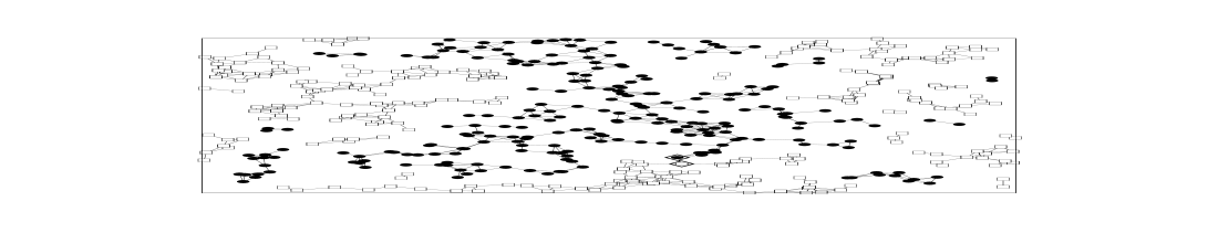
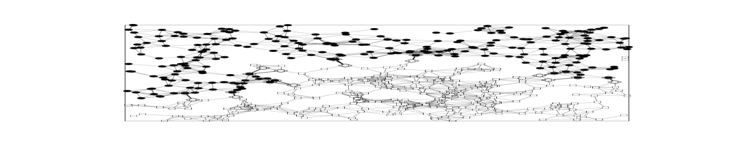
Figure 1: Two random geometric graphs, $n=500$, with connectivity 4 (top) and connectivity 8 (bottom) in an optimized configuration found by EO. At $\alpha=4$ the graph barely “percolates,” with merely one “bad” edge (between points of opposite sets, masked by diamonds) connecting a set of 250 round points with a set of 250 square points. For the denser graph on the bottom, EO reduced the cutsize to 13. A 1-$exchange$ will turn a square vertex into a round one, and a round vertex into a square one.

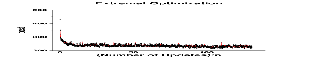
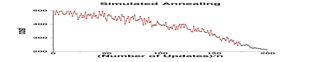
Figure 2: Evolution of the cost function $C(S)$ during a typical run of EO (left) and SA (right) for the bipartitioning of an $n=500$-vertex graph $G_{500}$ introduced in Ref. [38]. The best cost ever found for $G_{500}$ is 206. In contrast to SA, which has large fluctuations in early stages of the run and then converges much later, extremal optimization quickly approaches a stage where broadly distributed fluctuations allow it to probe and escape many local minima.

3.1 $\tau$-EO Algorithm

Tests have shown that this basic algorithm is very competitive for optimization problems where EO can choose randomly among many $S^{\prime}\in N(S)$ that satisfy step (2c) such as for the GBP [14]. But, as we will see below, sometimes the neighborhood $N$ chosen for a problem turns EO into a deterministic process: selecting always the worst variable in step (2b) leaves no choice in step (2c). Like iterative improvement, such an EO-process would get stuck in local minima. To avoid these “dead ends,” and to improve results generally[14], we introduce a single parameter into the algorithm. This parameter, $\tau$, remains fixed during each run and varies for each problem only with the system size $n$.

The parameter $\tau$ allows us to exploit the memory contained in the fitness ranking for the $x_{i}$ in more detail. We find a permutation $\Pi$ of the labels $i$ with

$$\lambda_{\Pi(1)}\leq\lambda_{\Pi(2)}\leq\ldots\leq\lambda_{\Pi(n)}.$$ (2)

The worst variable $x_{j}$ [step (2b)] is of rank 1, $j=\Pi(1)$, and the best variable is of rank $n$. Now, consider a probability distribution over the ranks $k$,

$$P_{k}\propto k^{-\tau},\qquad 1\leq k\leq n,$$ (3)

for a given value of the parameter $\tau$. At each update, select a rank $k$ according to $P_{k}$. (For sufficiently large $\tau$, this procedure will again select the vertex with the worst fitness, $k=1$, but for any finite $\tau$, it will occasionally dislodge fitter variables, $k>1$.) Then, modify step (2b) so that the variable $x_{j}$ with $j=\Pi(k)$ gets chosen for an update in step (2c). For example, in the case of the GBP with a 1-$exchange$, we now select two numbers $k_{1}$ and $k_{2}$ according to $P_{k}$ and swap vertex $j_{1}=\Pi(k_{1})$ with vertex $j_{2}=\Pi(k_{2})$ (we repeat drawing $k_{2}$ until $j_{1}$ and $j_{2}$ are from opposite sets).

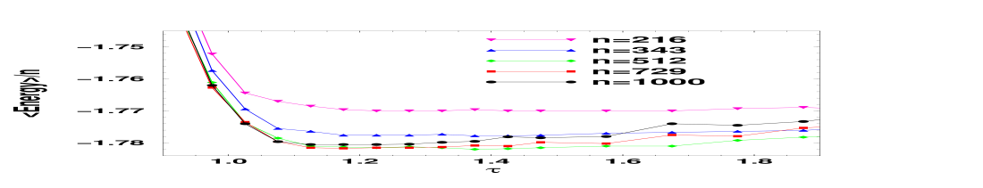
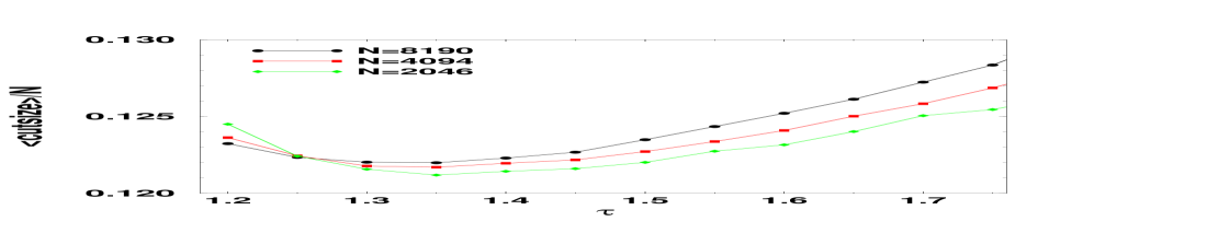
Figure 3: Plot of the average costs obtained by EO for a $\pm J$ spin glass (left) and for graph bipartitioning (right), as a function of $\tau$. For each size $n$, a number of instances were generated. For each instance, 10 different EO runs were performed at each $\tau$. The results were averaged over runs and over instances. Although both problems are quite distinct, in either case the best results are obtained for $\tau\to 1^{+}$ for $n\to\infty$.

For $\tau=0$, this “$\tau$-EO” algorithm is simply a local random walk through $\Omega$. Conversely, for $\tau\to\infty$, the process can approach a deterministic local search, only updating the lowest-ranked variable(s), and may be bound to reach a dead end (see Fig. 3). In both extremes the results are typically poor. However, for intermediate values of $\tau$ the choice of a (scale-free) power-law distribution for $P_{k}$ in Eq. (3) ensures that no rank gets excluded from further evolution, while still maintaining a bias against variables with bad fitness. As we will show in the next section, the $\tau$-EO algorithm can be analyzed to show that an asymptotic choice of $\tau-1\sim[\ln(n)]^{-1}$ optimizes the performance of the $\tau$-EO algorithm [11], which has been verified in the problems studied so far [16, 22, 15] as exemplified in Fig. 3.

3.2 Theory of the EO Algorithm

Stochastic local search heuristics are notoriously hard to analyze. Some powerful results have been derived for the convergence properties of SA in dependence of its temperature schedule [27, 2], based on the well-developed knowledge of equilibrium statistical physics (“detailed balance”) and Markov processes. But predictions for particular optimization problems are few and far between. Often, SA and GA, for instance, are analyzed on simplified models (see Refs. [44, 54, 19] for SA and Ref. [57] for GA) to gain insight into the workings of a general-purpose heuristic. We have studied EO on an appropriately designed model problem and were able to reproduce many of the properties observed for our realistic $\tau$-EO implementations. In particular, we found analytical results for the average convergence as a function of $\tau$ [11].

In Ref. [11] we have considered a model consisting of $n$ a-priori independent variables. Each variable $i$ can take on only one of, say, three fitness states, $\lambda_{i}=0$, -1, an -2, respectively assigned to fractions $\rho_{0}$, $\rho_{1}$, and $\rho_{2}$ of the variables, with the optimal state being $\lambda_{i}=0$ for all $1\leq i\leq n$, i. e. $\rho_{0}=1$, $\rho_{1,2}=0$ and cost $C=-\sum_{i}\lambda_{i}/n=\sum_{\alpha=0}^{2}\alpha\rho_{\alpha}=0$, according to Eq. (1). With this system, we can model the dynamics of local search for hard problems by “designing” an interesting set of flow equations for ${\bf\rho}(t)$ which can mimic a complex search space through energetic or entropic barriers, for instance [11]. These flow equations specify what fraction of variables transfer from on fitness state to another given that a variable in a certain state is updated. The update probabilities are easily derived for $\tau$-EO, giving a highly nonlinear dynamic system. Other local searchs may be studied in this model for comparison [10].

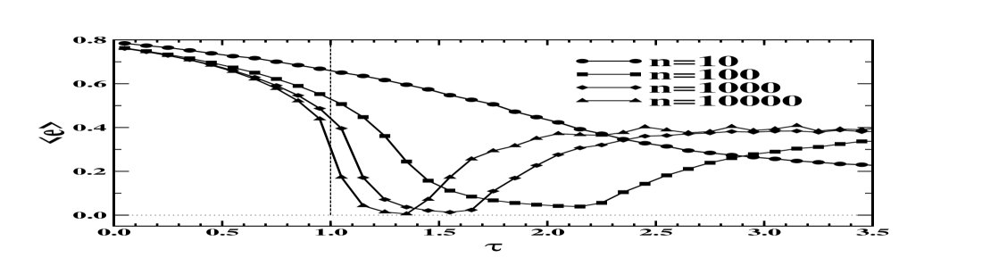
Figure 4: Plot of the cost $\left<C\right>$ averaged over many $\tau$-EO runs as a function of $\tau$ for $n=10$, 100, 1000, and 10000 from Ref. [11]. It reaches a minimum with $\left<C\right>\approx 0$ at a value near the prediction for $\tau_{\rm opt}\approx 3.5$, 2.1, 1.6, and 1.4 [from Eq. (4) with $A\approx 4$ and higher-order corrections], and rises sharply beyond that, similar to empirical findings, see Figs. 3a-b.

A particular design that allows the study of $\tau$-EO for a generic feature of local search is suggested by the close analogy between optimization problems and the low-temperature properties of spin glasses [47]: After many update steps most variables freeze into a near-perfect local arrangement and resist further change, while a finite fraction remains frustrated in a poor local arrangement [51]. More and more of the frozen (slow) variables have to be dislocated collectively to accommodate the frustrated (fast) variables before the system as a whole can improve its state. In this highly correlated state, slow variables block the progression of fast variables, and a “jam” emerges. And our asymptotic analysis of the flow equations for a jammed system indeed reproduces key features previously conjectured for EO from the numerical data for real optimization problems. Especially, it predicts for the value $\tau$ at which the cost is minimal for a given runtime,

$$\tau_{\rm opt}\sim 1+{A\over\ln n}\quad(n\to\infty),$$ (4)

where $A>0$ is some implementation specific constant. This result was found empirically before in Refs. [16, 15]. The behavior of the average cost $\left<C\right>$ as a function of $\tau$ for this model is shown in Fig. 4, which verifies Eq. (4).

This model provides the ideal setting to probe deeper into the properties of EO, and to compare it with other local search methods. Similarly, EO can be analyzed in terms of a homogeneous Markov chain [24, 37], although little effort has been made in this direction yet (except for Ref. [55]). Such theoretical investigations go hand-in-hand with the experimental studies to provide a clearer picture of the capabilities of EO.

3.3 Comparison with other Heuristics

As part of this project, we will often compare or combine EO with Meta-heuristics [49] and problem specific methods [5]. (This is also an important part of the educational purpose of this proposal.) As we will show, EO provides an alternative philosophy to the canon of heuristics. But these distinctions do not imply that any of the methods are fundamentally better or worse. To the contrary, their differences improve the chances that at least one of the heuristics will provide good results on some particular problem when all others fail! At times, best results are obtained by hybrid heuristics [52, 56, 53]. The most apparent distinction between EO and other methods is the need to define local cost contributions for each variable, instead of only a global cost. EO’s capability seems to derive from its ability to access this local information directly.

Simulated Annealing (SA): SA [42] emulates the behavior of frustrated systems in thermal equilibrium: if one couples such a system to a heat bath of adjustable temperature, by cooling the system slowly one may come close to attaining a state of minimal energy (i. e. cost). SA accepts or rejects local changes to a configuration according to the Metropolis algorithm [46] at a given temperature, enforcing equilibrium dynamics (“detailed balance”) and requiring a carefully tuned “temperature schedule” [1, 2]

In contrast, EO drives the system far from equilibrium: aside from ranking, it applies no decision criteria, and new configurations are accepted indiscriminately. Instead of tuning a schedule of parameters, EO often requires few choices. It may appear that EO’s results should resemble an ineffective random search, similar to SA at a fixed but finite temperature [23, 25]. But in fact, by persistent selection against the worst fitnesses, EO quickly approaches near-optimal solutions. Yet, large fluctuations remain at late runtimes (unlike in SA, see Fig. 2 or Ref. [38]) to escape deep local minima and to access new regions in configuration space.

In some versions of SA, low acceptance rates near freezing are circumvented using a scheme of picking trials from a rank-ordered list of possible moves [31] (see Chap. 2.3.4 in Ref. [53]), derived from continuous-time Monte Carlo methods [17]. Like in EO, every move gets accepted. But these moves are based on an outcome-oriented ranking, favoring downhill moves but permitting (Boltzmann-)limited uphill moves. On the other hand, in EO the ranking of variables is based on the current, not the future, state of each variable, allowing for unlimited uphill moves.

Genetic Algorithms (GA): Although similarly motivated by evolution (with deceptively similar terminology, such as “fitness”), GA [35, 29] and EO algorithms have hardly anything in common. GAs, mimicking evolution on the genotypical level, keep track of entire “gene pools” of configurations and use many tunable parameters to select and “breed” an improved generation of solutions. By comparison, EO, based on competition at the phenomenological level of “species,” operates only with local updates on a single configuration, with improvements achieved by persistent elimination of bad variables. EO, SA, and other general-purpose heuristics use a local search. In contrast, in GA cross-over operators perform global exchanges on a pair of configurations.

Tabu-Search (TS): TS performs a memory-driven local search procedure that allows for limited uphill moves based on scoring recent moves [28, 53, 3]. Its memory permits escapes from local minima and avoids recently explored configurations. It is similar to EO in that it may not converge ($S_{\rm best}$ has to be kept!), and that moves are ranked. But the uphill moves in TS are limited by tuned parameters that evaluate the memory. And, as for SA above, rankings and scoring of moves in TS are done on the basis of anticipated outcome, not on current “fitness” of individual variables.

4 EO-Implementations and Results

We have conducted a whole series of projects to demonstrate the capabilities of simple implementations in obtaining near-optimal solutions for the GBP [14, 16, 8], the 3-coloring of graphs [15, 12], and the Ising spin-glass problem [15] (a model of disordered magnets that maps to a MAX-CUT problem [39]). In each case we have studied a statistically relevant number of instances from an ensemble with up to $10^{4}$ variables, chosen from “Where the really hard problems are” [4]. These results are discussed in the following.

4.1 Graph Bipartitioning

In Table 1 we summarize early results of our $\tau$-EO implementation for the GBP on a testbed of graphs with $n$ as large as $10^{5}$. Here, we use $\tau=1.4$ and the best-of-10 runs. On each graph, we used as many update steps $t$ as appeared productive for EO to reliably obtain stable results. This varied with the particularities of each graph, from $t=2n$ to $200n$, and the reported runtimes are influenced by this.

Table 1: Best cutsizes (and allowed runtime) for a testbed of large graphs. GA results are the best reported [45] (at 300MHz). $\tau$-EO results are from our runs (at 200MHz), out-pacing the GA results by almost an order of magnitude for large $n$ . Comparison data for three of the large graphs are due to results from spectral heuristics in Ref. [33] (at 50MHz). METIS is a partitioning program based on hierarchical reduction instead of local search [41], obtaining extremely fast deterministic results (at 200MHz).

Large Graph $n$		GA		$\tau$-EO		Ref. [33]		p-METIS
Hammond	4720	90	(1s)	90	(42s)	97	(8s)	92	(0s)
Barth5	15606	139	(44s)	139	(64s)	146	(28s)	151	(0.5s)
Brack2	62632	731	(255s)	731	(12s)	—		758	(4s)
Ocean	143437	464	(1200s)	464	(200s)	499	(38s)	478	(6s)

In an extensive numerical study on random and geometric graphs [8] we have shown that $\tau$-EO outperforms SA significantly near phase transitions, where cutsizes first become non-zero. To this end, we have compared the averaged best results obtained for both methods for a large number of instances for increasing $n$ at a fixed parameter setting. For EO, we have used the algorithm for GBP described in Sec. 3.1 at $\tau=1.4$. For SA, we have used the algorithm developed by Johnson [38] for GBP, with a geometric temperature schedule and a temperature length of $64n$ to equalize runtimes between EO and SA. Both programs used the same data structure, with EO requiring a small extra overhead for sorting the fitness of variables in a heap [14]. Clearly, since each update leads to a move and entails some sorting, individual EO updates take much longer than an SA trial step. Yet, as Fig. 5 shows, SA gets rapidly worse near the phase transition relative to EO, at equalized CPU-time.

Figure 5: Plot of the error in the best result of SA relative to EO’s on identical instances of random graphs (left) and geometric graphs (right) as function of the average connectivity $c$. The critical points for the GBP are at $c=2\ln 2=1.386$ for random graphs and at $c\approx 4.5$ for geometric graphs. SA’s error relative to EO near the critical point in both cases rises with $n$.

Studies on the average rate of convergence toward better-cost configurations as a function of runtime $t$ indicate power-law convergence, roughly like $\left<C(S_{\rm best})\right>_{t}\sim\left<C(S_{\rm min})\right>+A\,t^{-0.4}$ [16], also found by Ref. [22]. Of course, it is not easy to assert for graphs of large $n$ that those runs in fact converge closely to the optimum $C(S_{\rm min})$, but finite-size scaling analysis for random graphs justifies that expectation [16].

4.2 Graph Coloring

An instance in graph coloring consists of a graph with $n$ vertices, some of which are connected by edges, just like in the GBP. We have considered the problem of MAX-$K$-COL: given $K$ different colors to label the vertices, find a coloring of the graph that minimizes the number of “monochromatic” edges that connect vertices of identical color.

For MAX-$K$-COL we define the fitness as $\lambda_{i}=-b_{i}/2$, like for the GBP, where $b_{i}$ is the number of monochromatic edges emanating from vertex $i$. Since there are no global constraints, a simple random reassignment of a new color to the selected variable $x_{j}$ is a sufficient local-search neighborhood.

We have studied the MAX-3-COL problem near its phase transition, where the hardest instances reside [36, 18, 21, 4]. In Ref. [18] the phenomena of phase transition has been studied first for $3$- and $4$-COL. Here, we used EO to completely enumerate all optimal solutions $S_{\rm min}$ near the critical point for $3$-COL of random graphs. Instances of random graphs typically have a high ground-state degeneracy, i. e. possess a large number of equally optimal solutions $S_{\rm min}$. In Ref. [48] it was shown that at the phase transition of $3$-SAT the fraction of constrained variables, i. e. those that are found in an identical state in almost all $S_{\rm min}$, discontinuously jumps to a non-zero value. It was conjectured that this first-order phase transition in this “backbone” is a general phenomenon for NP-hard optimization problems.

To test the conjecture for the 3-COL, we generated a large number of random graphs and explored $\Omega$ for as many ground states as EO could find. (We fixed runtimes well above the times needed to saturate the set of all $S_{\rm min}$ in repeated trials on a testbed of exactly known instances.) For each instance, we measured the optimal cost and the backbone fraction of fixed pairs of vertices. The results in Fig. 6 allow us to estimate precisely the location of the transition and the scaling behavior of the cost function. With a finite-size scaling ansatz to “collapse” the data for the average ground-state cost onto a single scaling curve,

$$\left<C\right>\sim nf\left[\left(c-c_{\rm crit}\right)n^{1/\nu}\right],$$ (5)

it is possible to extract precise estimates for the location of the transition $c_{\rm crit}$ and the scaling window exponent $\nu$.

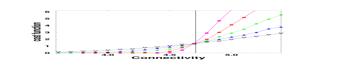
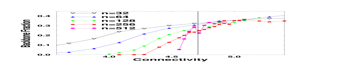
Figure 6: Plot of the average cost (left) and of the backbone fraction (right) as a function of the average connectivity $c$ for random graph 3-coloring. The data collapse according to Eq. (5) in the insert on the left predicts a critical point for random graphs at $c_{\rm crit}\approx 4.72$ (indicated by a vertical line) and $\nu=1.53(5)$. We generated at each value of $c$ $10000$, $5000$, $1300$, $650$, and $150$ instances for $n=32$, 64, 128, 256, and 512, respectively.

4.3 “Spin Glasses” (or MAX-CUT)

Of significant physical relevance are the low temperature properties of “spin glasses” [47], which are closely related to MAX-CUT problems [39]. EO was originally designed with applications to spin glasses in mind, and some of its most successful results were obtained for such systems [15]. Many physical and classic combinatorial optimization problems (Matching, Partitioning, Satisfiability, or the Integer Programming problem below) can be cast in terms of a spin glass [47].

A spin glass consists of a lattice or a graph with a spin variable $x_{i}\in\{-1,1\}$ placed on each vertex $i$, $1\leq i\leq n$. Every spin is connected to each of its nearest neighbors $j$ via a fixed bond variable $J_{i,j}$, drawn at random from a distribution of zero mean and unit variance. Spins may be coupled to an arbitrary external field $h_{i}$. The optimization problem consists of finding minimum cost states $S_{\rm min}$ of the “Hamiltonian”

$$C(S)=H(x_{1},\ldots,x_{n})=-{1\over 2}\sum_{i,j}J_{i,j}x_{i}x_{j}-\sum_{i}x_{i}h_{i}.$$ (6)

Arranging spins into an optimal configuration is hard due to “frustration:” variables that will, individually or collectively, never be able to satisfy all constraints imposed on them. The cost function in Eq. (6) is equivalent to integer quadratic programming problems [39].

We simply define as fitness the local cost contribution for each spin,

$$\lambda_{i}=x_{i}\left({1\over 2}\sum_{j}J_{i,j}x_{j}+h_{i}\right),$$ (7)

and Eq. (6) turns into Eq. (1). A single spin flip provides a sufficient neighborhood for this problem. This formulation trivially extends to higher than quadratic couplings.

We have run this EO implementation for a spin glass with $h_{i}\equiv 0$ and random $J_{i,j}=\pm 1$ for nearest-neighbor bonds on a cubic lattice [15]. We used $\tau=1.15$ on a large number of realizations of the $J_{ij}$, for $n=L^{3}$ with $L=5,6,7,8,9,10,12$. For each instance, we have run EO with 5 restarts from random initial conditions, retaining only the lowest energy state obtained, and then averaging over instances. Inspection of the results for convergence of the genetic algorithms in Refs. [50, 34] suggest a computational cost per run of at least $O(n^{3}--n^{4})$ for consistent performance. Indeed, using $\sim n^{4}/100$ updates enables EO to reproduce its lowest energy states on about 80% to 95% of the restarts, for each $n$. Our results are listed in Tables 2. A fit of our data for the energy per spin, $e(n)=<C>_{n}/n$, $C(s)$ defined in Eq. (6), with $e(n)=e(\infty)+{\rm const}/n$ for $n\to\infty$ predicts $e(\infty)=1.7865(3)$, consistent with the findings of Refs. [50, 32], providing independent confirmation of those results with far less parameter tuning.

Table 2: EO approximations to the average ground-state energy per spin $e(n)$ of the $\pm J$ spin glass in $d=3$, compared with GA results from Refs. [50, 32]. For each size $n=L^{3}$ we have studied a large number $I$ of instances. Also shown is the average time $t$ (in seconds) needed for EO to find the presumed ground state on a 450MHz Pentium. (As for a normal distribution, for increasing $n$ fewer instances are needed to obtain similar error bars.)

$L$	$I$	$e(n)$	$t$	Ref. [50]	Ref. [32]
3	40100	-1.6712(6)	0.0006	-1.67171(9)	-1.6731(19)
4	40100	-1.7377(3)	0.0071	-1.73749(8)	-1.7370(9)
5	28354	-1.7609(2)	0.0653	-1.76090(12)	-1.7603(8)
6	12937	-1.7712(2)	0.524	-1.77130(12)	-1.7723(7)
7	5936	-1.7764(3)	3.87	-1.77706(17)
8	1380	-1.7796(5)	22.1	-1.77991(22)	-1.7802(5)
9	837	-1.7822(5)	100.
10	777	-1.7832(5)	424.	-1.78339(27)	-1.7840(4)
12	30	-1.7857(16)	9720.	-1.78407(121)	-1.7851(4)

To gauge EO’s performance for larger $n$, we have run our implementation also on two $3d$ lattice instances, $toruspm$3-8-50 and $toruspm$3-15-50, with $n=8^{3}$ and $n=15^{3}$, considered in the 7th DIMACS challenge for semi-definite problems [39]. Bounds [40] on the ground-state cost established for the larger instance are $C_{\rm lower}=-6138.02$ (from semi-definite programming) and $C_{\rm upper}=-5831$ (from branch-and-cut). EO found $C(S_{\rm best})=-6049$ (or $e=C/n=-1.7923$), a significant improvement on the upper bound and already lower than $e(\infty)$ from above. Furthermore, we collected $10^{5}$ such states, which roughly segregate into 3 clusters with a mutual Hamming distance of at least 100 distinct spins. For the smaller instance the bounds given are -922 and -912, resp., while EO finds -916 (or $C/n=-1.7891$). While this run (including sampling degenerate states!) took only a few minutes of CPU (at 800MHz), the results for the larger instance require about 16 hours.

1

References

- [1] E. H. L. Aarts and P. J. M. van Laarhoven, Statistical Cooling: A general Approach to Combinatorial Optimization Problems, Philips J. Res. 40, 193-226 (1985).
- [2] E. H. L. Aarts and P. J. M. van Laarhoven, Simulated Annealing: Theory and Applications (Reidel, Dordrecht, 1987).
- [3] Local Search in Combinatorial Optimization, Eds. E. H. L. Aarts and J. K. Lenstra (Wiley, New York, 1997).
- [4] See Frontiers in problem solving: Phase transitions and complexity, eds. T. Hogg, B. A. Huberman, and C. Williams, special issue of Artificial Intelligence 81:1–2 (1996).
- [5] G. Ausiello et al., Complexity and Approximation (Springer, Berlin, 1999).
- [6] P. Bak and K. Sneppen, Punctuated Equilibrium and Criticality in a simple Model of Evolution, Phys. Rev. Lett. 71, 4083-4086 (1993).
- [7] P. Bak, C. Tang, and K. Wiesenfeld, Self-Organized Criticality, Phys. Rev. Lett. 59, 381-384 (1987).
- [8] S. Boettcher, Extremal Optimization and Graph Partitioning at the Percolation Threshold, J. Math. Phys. A: Math. Gen. 32, 5201-5211 (1999).
- [9] S. Boettcher, Extremal Optimization: Heuristics via Co-Evolutionary Avalanches, Computing in Science and Engineering 2:6, 75 (2000).
- [10] S. Boettcher and M. Frank, Analysis of Extremal Optimization in Designed Search Spaces, Honors Thesis, Dept. of Physics, Emory University, (in preparation).
- [11] S. Boettcher and M. Grigni, Jamming model for the extremal optimization heuristic, J. Phys. A: Math. Gen. 35 1109-1123 (2002).
- [12] S. Boettcher, M. Grigni, G. Istrate, and A. G. Percus, Phase Transitions and Algorithmic Complexity in 3-Coloring, (in preparation).
- [13] S. Boettcher and A. G. Percus, Extremal Optimization: Methods derived from Co-Evolution, in GECCO-99: Proceedings of the Genetic and Evolutionary Computation Conference (Morgan Kaufmann, San Francisco, 1999), 825-832.
- [14] S. Boettcher and A. G. Percus, Nature’s Way of Optimizing, Artificial Intelligence 119, 275-286 (2000).
- [15] S. Boettcher and A. G. Percus, Optimization with Extremal Dynamics, Phys. Rev. Lett. 86, 5211-5214 (2001).
- [16] S. Boettcher and A. G. Percus, Extremal Optimization for Graph Partitioning, Phys. Rev. E 64, 026114 (2001).
- [17] A. B. Bortz, M. H. Kalos, and J. L. Lebowitz, J. Comp. Phys. 17, 10-18 (1975).
- [18] P. Cheeseman, B. Kanefsky, and W. M. Taylor, Where the really hard Problems are, in Proc. of IJCAI-91, eds. J. Mylopoulos and R. Rediter (Morgan Kaufmann, San Mateo, CA, 1991), pp. 331–337.
- [19] H. Cohn and M. Fielding, Simulated Annealing: Searching for an optimal Temperature Schedule, SIAM J. Optim. 9, 779-802 (1999).
- [20] S. A. Cook, The Complexity of Theorem-Proving Procedures, in: Proc. 3rd Annual ACM Symp. on Theory of Computing, 151-158 (Assoc. for Computing Machinery, New York, 1971).
- [21] J. Culberson and I. P. Gent, Frozen Development in Graph Coloring, J. Theor. Comp. Sci. 265, 227-264 (2001).
- [22] J. Dall, Searching Complex State Spaces with Extremal Optimization and other Stochastics Techniques, Master Thesis, Fysisk Institut, Syddansk Universitet Odense, 2000 (in danish).
- [23] J. Dall and P. Sibani, Faster Monte Carlo Simulations at Low Temperatures: The Waiting Time Method, Computer Physics Communication 141, 260-267 (2001).
- [24] W. Feller, An Introduction to Probability Theory and Its Applications, Vol. 1 (Wiley, New York, 1950).
- [25] M. Fielding, Simulated Annealing with an optimal fixed Temperature, SIAM J. Optim. 11, 289-307 (2000).
- [26] M. R. Garey and D. S. Johnson, Computers and Intractability, A Guide to the Theory of NP-Completeness (W. H. Freeman, New York, 1979).
- [27] S. Geman and D. Geman, Stochastic Relaxation, Gibbs Distributions, and the Bayesian Restoration of Images, in Proc. 6th IEEE Pattern Analysis and Machine Intelligence, 721-741 (1984).
- [28] F. Glover, Future Paths for Integer Programming and Links to Artificial Intelligence, Computers & Ops. Res. 5, 533-549 (1986).
- [29] D. E. Goldberg, Genetic Algorithms in Search, Optimization, and Machine Learning, (Addison-Wesley, Reading, 1989).
- [30] S. J. Gould and N. Eldridge, Punctuated Equilibria: The Tempo and Mode of Evolution Reconsidered, Paleobiology 3, 115-151 (1977).
- [31] J. W. Greene and K. J. Supowit, Simulated Annealing without rejecting moves, IEEE Trans. on Computer-Aided Design CAD-5, 221-228 (1986).
- [32] A. K. Hartmann, Evidence for existence of many pure ground states in 3d Spin Glasses, Europhys. Lett. 40, 429 (1997).
- [33] B. A. Hendrickson and R. Leland, A multilevel algorithm for partitioning graphs, in: Proceedings of Supercomputing ’95, San Diego, CA (1995).
- [34] J. Houdayer and O. C. Martin, Renormalization for discrete optimization, Phys. Rev. Lett. 83, 1030-1033 (1999).
- [35] J. Holland, Adaptation in Natural and Artificial Systems (University of Michigan Press, Ann Arbor, 1975).
- [36] B. A. Huberman and T. Hogg, Phase transitions in artificial intelligence systems, Artificial Intelligence 33, 155-171 (1987).
- [37] M. Jerrum and A. Sinclair, The Markov chain Monte Carlo method: an approach to approximate counting and integration, in Approximation Algorithms for NP-hard Problems, ed. Dorit Hochbaum (PWS Publishers, 1996).
- [38] D. S. Johnson, C. R. Aragon, L. A. McGeoch, and C. Schevon, Optimization by Simulated Annealing - an Experimental Evaluation. 1. Graph Partitioning, Operations Research 37, 865-892 (1989).
- [39] 7th DIMACS Implementation Challenge on Semidefinite and related Optimization Problems, eds. D. S. Johnson, G. Pataki, and F. Alizadeh (to appear, see http://dimacs.rutgers.edu/Challenges/Seventh/).
- [40] M. Jünger and F. Liers (Cologne University), private communication.
- [41] G. Karypis and V. Kumar, METIS, a Software Package for Partitioning Unstructured Graphs, see http://www-users.cs.umn.edu/~karypis/metis/main.shtml, (METIS is copyrighted by the Regents of the University of Minnisota).
- [42] S. Kirkpatrick, C. D. Gelatt, and M. P. Vecchi, Optimization by simulated annealing, Science 220, 671-680 (1983).
- [43] S. Kirkpatrick and B. Selman, Critical Behavior in the Satisfiability of Random Boolean Expressions, Science 264, 1297-1301 (1994).
- [44] M. Lundy and A. Mees, Convergence of an Annealing Algorithm, Math. Programming 34, 111-124 (1996).
- [45] P. Merz and B. Freisleben, Memetic algorithms and the fitness landscape of the graph bi-partitioning problem, Lect. Notes Comput. Sc. 1498, 765-774 (1998).
- [46] N. Metropolis, A.W. Rosenbluth, M.N. Rosenbluth, A.H. Teller and E. Teller, Equation of state calculations by fast computing machines, J. Chem. Phys. 21 (1953) 1087–1092.
- [47] M. Mezard, G. Parisi, and M. A. Virasoro, Spin Glass Theory and Beyond (World Scientific, Singapore, 1987).
- [48] R. Monasson, R. Zecchina, S. Kirkpatrick, B. Selman, and L. Troyansky, Determining computational complexity from characteristic ’phase transitions,’ Nature 400, 133-137 (1999), and Random Struct. Alg 15, 414-435 (1999).
- [49] Meta-Heuristics: Theory and Application, Eds. I. H. Osman and J. P. Kelly (Kluwer, Boston, 1996).
- [50] K. F. Pal, The ground state energy of the Edwards-Anderson Ising spin glass with a hybrid genetic algorithm, Physica A 223, 283-292 (1996).
- [51] R. G. Palmer, D. L. Stein, E. Abrahams, and P. W. Anderson, Models of Hierarchically Constrained Dynamics for Glassy Relaxation, Phys. Rev. Lett. 53, 958-961 (1984).
- [52] Modern Heuristic Search Methods, Eds. V. J. Rayward-Smith, I. H. Osman, and C. R. Reeves (Wiley, New York, 1996).
- [53] Modern Heuristic Techniques for Combinatorial Problems, Ed. C. R. Reeves (Wiley, New York, 1993).
- [54] G. B. Sorkin, Efficient Simulated Annealing on Fractal Energy Landscapes, Algorithmica 6, 367-418 (1991).
- [55] D. E. Vaughan and S. H. Jacobson, Nonstationary Markov Chain Analysis of Simultaneous Generalized Hill Climbing Algorithms, (submitted), available at http:// filebox.vt.edu/users/dvaughn/pdf_powerpoint/sghc2.pdf.
- [56] Meta-Heuristics: Advances and Trends in Local Search Paradigms for Optimization, Ed. S. Voss (Kluwer, Dordrecht, 1998).
- [57] I. Wegener, Theoretical aspects of evolutionary algorithms, Lecture Notes in Computer Science 2076, 64-78 (2001).