Analysis of Non-Gaussian Nature of Network Traffic and its Implication on Network Performance

Abstract

We analyzed the non-Gaussian nature of network traffic using some Internet traffic data. We found that (1) the non-Gaussian nature degrades network performance, (2) it is caused by ‘greedy flows’ that exist with non-negligible probability, and (3) a large majority of ‘greedy flows’ are TCP flows having relatively small hop counts, which correspond to small round-trip times. We conclude that in a network that has greedy flows with non-negligible probability, a traffic controlling scheme or bandwidth design that considers non-Gaussian nature is essential.

1 Introduction

Traffic characterization based on measurements is crucial for establishing high-quality performance evaluation and efficient network provisioning. It has been widely elucidated that in today’s high-speed data networks, self-similarity is appropriate for traffic characterization and performance evaluation since pioneering work conducted by researchers from Bellcore in the early 1990s [6, 9]. Self-similarity in data network traffic suggests that traffic variability has ‘long-range dependence (LRD)’, while the classic Poisson traffic model is based on the principle that traffic variability has short-range dependence (exponential). In a series of self-similarity related studies, it was found that if traffic variability has a higher degree of LRD, then network performance tends to be worse than when it has a lower one [7, 8, 9].

Self-similarity in data networks has been studied in terms of its ubiquitous presence and usefulness from various measurements and statistical analyses and simulation studies. However, these are not sufficient from the viewpoint of evaluating network performance. That is, in some cases network traffic with a higher degree of LRD could show better performance than that with a lower one — the reverse of above findings. This is because LRD reflects only the temporal structure of traffic variability and not its spatial structure, such as marginal distribution. Grossglauser et al. showed, using a fluid traffic model [3], that in addition to LRD, the difference in marginal distributions strongly affect network performance. However, detailed information about marginal distributions of real network traffic and the way to describe them in their fluid traffic model was not given in the study. In general, if traffic is aggregated from a number of independent and identically distributed flows, the marginal distribution of its variability is considered to be Gaussian and this nature is guaranteed by the central limit theorem. Actually, in recent traffic models that reflect traffic LRD such as the well known fractional Brownian motion traffic model proposed by Norros [7] or the one proposed by Willinger and Taqqu [16], which is a superposition of a large number of independent ON/OFF sources with heavy-tailed ON and/or OFF periods, their marginal distribution of traffic variability is Gaussian.

In this paper, we investigate marginal distributions of network traffic using some Internet traffic data. We found that marginal distributions of traffic variability are not always Gaussian (i.e., they are non-Gaussian) and in many cases, they are skewed positively. We also show that the non-Gaussian nature has a strong influence on network performance. This means that it is essential to consider the non-Gaussian nature of network traffic in order to characterize traffic variability. Thus, we focus on the mechanisms that cause non-Gaussian nature of traffic variability. To study this, we analyze the behavior of each IP flow composing aggregated traffic from the viewpoints of size distribution, hop counts, RTT, and protocol.

This paper is organized as follows. Section 2 shows examples of the non-Gaussian nature of network traffic and its implication on network performance. In section 3, to identify the mechanisms causing non-Gaussian nature, we define ‘per-time-unit flow’ and analyze its statistics such as size distribution, hop counts, RTT, and protocol. Section 4 gives our conclusions.

2 Examples of Non-Gaussian Nature and performance implication

This section shows examples of the non-Gaussian nature of network traffic using real Internet traffic traces and then shows its performance implications by trace driven simulation.

2.1 Data

We used traces from three different sets of network traffic for our analyses. In this work, the length of all traces was set to 300 s to avoid the effect of non-stationarity and also to get enough statistics. Actually, each trace had at least 100,000 packets in this condition. Details about the traces are briefly summarized as follows.

Data I: ECL external line

This line is the main external connection line of NTT R&D center (ECL). It is a 12-Mbps ATM line and traces were captured at the segment one hop before the line. The measurements were made during daily busy hours on some weekdays in July 2001. In total we used 48 traces for this study.

Data II: OCN-SINET

This line connects NTT’s Open Computer Network (OCN) and the Science Information Network (SINET). OCN is NTT’s commercial Internet backbone network and SINET is the largest Internet backbone network for scientific research institutes in Japan. The link is a 135-Mbps ATM line. The measurements were made during daily busy hours on some weekdays in January 2000. In total we used 34 traces for this study. More detailed information about this data is available in [5].

Data III: Bellcore

The lines are several Ethernet networks at the Bellcore Morristown Research and Engineering facility. Traces are available from the Internet Traffic Archive [13]. In this study, we used the first 300 s of BC-pAug89.TL. Detailed information about the traces is shown in [6], where the self-similarity of Ethernet traffic was first demonstrated using data that included this data set.

2.2 Traffic variability and marginal distributions

For all traces described in 2.1, we calculated the throughput variability and their marginal distributions. Here, we calculated throughput using a time interval of 0.1 s. Figure 1, shows throughput variability (left side) and marginal distributions (right side) for randomly chosen traces from the three networks described in 2.1. From this figure, we can intuitively find that marginal distributions of all traces are asymmetric and skewed positively. To characterize the difference in marginal distributions quantitatively, we used skewness, which is defined as

$$skewness=\frac{\left<\left(X-\left<X\right>\right)^{3}\right>}{\sigma^{3}},$$ (1)

where $\left<X\right>$ is the mean of $X$ and $\sigma$ is the standard deviation of $X$. If the distribution is skewed positively (negatively), skewness is positive (negative). If the distribution is exactly Gaussian, the shape of the marginal distribution is symmetric and the skewness is 0. Table 1 shows skewness of three example traces given in Fig. 1. All values of skewness took positive values. In these three example traces, we can see that traffic variability of Data III has the strongest non-Gaussian nature.

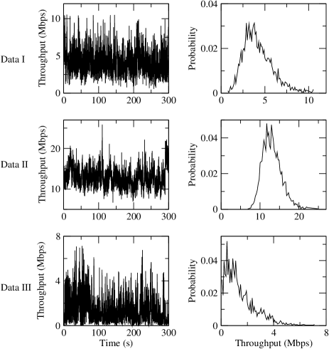
Figure 1: Examples of non-Gaussian nature of traffic variability.

Table 1: Skewness of three example traces.

	Data I	Data II	Data III
$skewness$	0.812	0.655	1.320

2.3 Non-Gaussian nature and network performance

For Data I and II, we performed trace-driven simulation to see the effect of non-Gaussian nature on network performance in conditions having similar bandwidth and buffer capacity. We used Internet-to-ECL traffic for Data I and OCN-to-SINET traffic for Data II because these directions have more traffic than the opposite directions. We did not use Data III because we could not clarify the direction of traffic from given traces.

We also show the relationship between the Hurst parameter and network performance for comparison. The Hurst parameter, $H$, is between 0.5 and 1, where a large value means a high degree of LRD [6],[9]. To estimate $H$, we employed power spectrum density estimation, removing the linear trend from the throughput time series before employing a Fourier transform (Fig. 2). From the slope $\alpha$ of the log-log regression of the power spectrum density versus the frequency, we get $H=\frac{1-\alpha}{2}$ [1],[12]. Here, the lowest 10% of frequency was used for regression. Table 2 shows estimated Hurst parameters of three example traces given in Fig. 1. All values are larger than 0.5, which indicates that all traces have LRD.

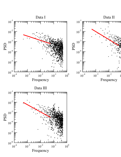
Figure 2: Power spectrum density for three traces given in Fig. 1.

Table 2: Estimated Hurst parameters of three example traces.

	Data I	Data II	Data III
$H$	0.714	0.894	0.858

Figure 3: Simulation environment.

Figure 3 shows our simulation model. As the network simulator, we used ns-2 [14]. The one-way trace data was set to ‘Trace source’ and packets were sent from it to ‘Trace sink’ via two nodes following the timestamp and packet size recorded in the trace data. In this study, there was no host-side traffic control scheme such as TCP; all packets were treated like UDP packets. This is because we wanted to see how packets would be discarded given a constrained bandwidth for originally demanded (non-shaped) traffic. Here, we set the buffer size of the ‘aggregation link’ to 50 packets to see the difference in performance clearly, and used FIFO as the packet scheduling. The link bandwidth was changed so that the link utilization of each trace was 0.6. For example, if the average traffic variability (throughput) of a trace was 6 Mbps, we set the bandwidth to 10 Mbps.

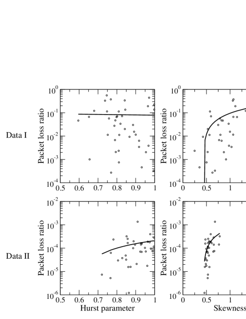
Figure 4: Results of trace-driven simulation. Left side shows Hurst parameter vs. packet loss ratio; right side shows skewness vs. packet loss ratio. Top is the result using Data I and bottom is Data II.

Table 3: Correlation coefficients of Hurst parameter and skewness vs. packet loss ratio.

	Data I	Data II
Hurst parameter	-0.015	0.169
skewness	0.584	0.435

For each trace, we calculated its skewness and Hurst parameter from its throughput variability, and performed the trace-driven simulation. Figure 4 shows the results where each point corresponds to the result of one trace. From the figure, we can see that both Hurst parameter and skewness took a wide range of values for two networks. That is, most of traffic had LRD and was positively skewed (non-Gaussian). It also shows that as skewness increased, network performance degraded as well. That is, as the non-Gaussian nature became stronger, the network performance became more degraded. To see the relationship between network performance and the above two characteristics (LRD, non-Gaussian) quantitatively, we calculated correlation coefficients between them (Table 3). In Fig. 4, solid lines indicate linear regression. The table shows that skewness was positively correlated with network performance while the Hurst parameter had little correlation with it. These results imply that the non-Gaussian nature of traffic strongly affects the network performance.

3 Mechanism of Non-Gaussian Nature

This section investigates the mechanism of the non-Gaussian nature of network traffic. For this, we first introduce ‘per-time-unit flow’ — an IP flow defined in a given time unit — to analyze the behavior of IP flows composing the aggregated traffic. Here IP flow is a group of packets having a unique combination of source IP address, destination IP address, source port, destination port, and protocol as is defined in [15, 5]. Then we show that ‘greedy flows’ strongly affect the non-Gaussian nature of network traffic. After that, we show the nature of greedy flows from the viewpoints of hop counts distributions. Investigating the relationship between traffic variability and hop count distributions will also enable us to establish efficient network bandwidth design according to its topology. To investigate the nature of greedy flows in detail, we also studied RTT and protocol distributions of per-time-unit flows.

3.1 Definition of per-time-unit flow and greedy flows

Many recent ON/OFF source traffic models (also known as packet train models) such as [16] and [8] assume that traffic is aggregated from a number of flows having a uniform rate. Accordingly, each flow has a similar size on a certain time scale when the flow is in the ON-period. It should also be pointed out that in these models, aggregated traffic shows the Gaussian nature according to the central limit theorem, as mentioned in section 1. However, it is not clear that the above “uniform rate assumption” is appropriate for modern Internet traffic. So we introduce ‘per-time-unit flow’ to investigate how traffic is aggregated on a certain time scale, and to see how the behavior of each flow contributes to the non-Gaussian nature of aggregated traffic.

In Fig. 5, each square corresponds to one IP flow. We divided traces into time unit $T_{i}$, where $1\leq i\leq M$. For all $i$, the length of $T_{i}$ was set to time interval $\tau$. For each $T_{i}$, we define per-time-unit flow $fl\_j\left(T_{i}\right)$ as shown by the shaded regions in the figure, where $1\leq j\leq N_{T_{i}}$ and $N_{T_{i}}$ is the number of flows during $T_{i}$. The per-time-unit flow $fl\_j\left(T_{i}\right)$ should contain at least two packets during $T_{i}$. In this work the length of $\tau$ was set to 0.1 s.

For each per-time-unit flow $fl\_j\left(T_{i}\right)$, we counted the number of packets $N_{p}\left(fl\_j\left(T_{i}\right)\right)$. In this study, we defined a ‘greedy flow’ as one whose $N_{p}\left(fl\_j\left(T_{i}\right)\right)$ is larger than 20, which corresponds to throughput of about 1 Mbps assuming the average packet size to be 700 bytes.

3.2 Size distribution of per-time-unit flow

For Data I and II, we investigated the size distribution of $N_{p}\left(fl\_j\left(T_{i}\right)\right)$. We calculated the following complementary cumulative distribution for all $i,j$.

$$P\left[N_{p}\left(fl\_j\left(T_{i}\right)\right)>n_{p}\right]$$ (2)

Figure 6 shows the log-log complementary cumulative distribution (LLCD) plots of $N_{p}\left(fl\_j\left(T_{i}\right)\right)$ for all $i,j$. As we can see immediately, the figure shows that distributions of $N_{p}\left(fl\_j\left(T_{i}\right)\right)$ are in good agreement with the power-law; that is,

$$P\left[N_{p}\left(fl\_j\left(T_{i}\right)\right)>n_{p}\right]\sim n_{p}^{-\alpha},\quad as\quad n_{p}\to\infty.$$ (3)

Figure 5: Definition of per-time-unit flow.

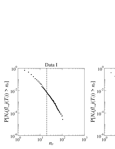
Figure 6: LLCD plots of $N_{p}\left(fl\_j\left(T_{i}\right)\right)$ for two traces given in Fig. 1.

Estimated power exponents $\alpha$ of equation (3) for traces given in Fig. 1 are 2.96 for Data I and 1.83 for Data II, where the regression range was set to $n_{p}\geq 10$. Correlation coefficients for regressions are -0.99 for both Data I and II. The power-law of distributions of $N_{p}\left(fl\_j\left(T_{i}\right)\right)$ indicates that both traces described in Fig. 6 had greedy flows with non-negligible probability (right side of the dashed line in the figure. It should also be pointed out that as $\alpha$ approaches 2, the distribution of $N_{p}\left(fl\_j\left(T_{i}\right)\right)$ approaches a heavy-tailed distribution, which indicates that very large values existed with non-negligible probability.

3.3 Greedy flows and non-Gaussian nature

In order to see the relationship between greedy flows and the non-Gaussian nature of network traffic, we investigated the relationship between estimated power exponents $\alpha$ of equation (3) and the skewness of throughput variability for each trace. In Fig. 7, the estimated power exponents $\alpha$ are plotted against skewness for all traces of Data I and II. The figure shows that in both cases, skewness increased as $\alpha$ decreased, and this tendency was stronger when $\alpha$ was close to 2 (inside ellipses and dashed lines). These results lead to the conclusion that greedy flows existing with non-negligible probability contribute to the non-Gaussian nature of network traffic, because the decrease in $\alpha$ corresponds to an increase in the probability of a greedy flow existing and the increase in skewness corresponds to an increase in the degree of non-Gaussian nature of network traffic.

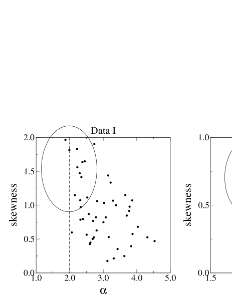
Figure 7: Exponents $\alpha$ vs. skewness. Left side is Data I and right side is Data II.

Figure 8: Hop count estimation between two hosts.

3.4 Hop count distribution of per-time-unit flow

For each per-time-unit flow $fl\_j\left(T_{i}\right)$, we investigated hop counts $hop\left(fl\_j\left(T_{i}\right)\right)$. We used only Data I because traces of Data II contain only one-way traffic and we could not estimate hop counts of each flow with our method described below. To study hop counts between two nodes from the given trace data, we used the TTL (time to live) field of an IP packet. As its value is decreased when an IP packet passes a router, we can estimate hop counts between the source node and measuring point from the initial TTL value and the TTL value of the received packet. So, if we can obtain the hop counts from both the source and destination nodes to the measuring point, we can estimate the hop counts between these nodes. We show an example below.

In Fig. 8, client C and server S compose an IP flow. Let initial TTL values of each host to be 128 and 64. If we obtain TTL values as 125 and 62 at the measuring point, hop counts between these two nodes can be estimated as $\left(128-125\right)+\left(64-62\right)+1=6$, where we assume that the route between two nodes does not change during a round-trip. One difficulty with this approach is that the initial TTL values depend on the operating system or network equipment such as routers (see [11] for example). To overcome this difficulty, we employed the technique introduced by Fujii et al. in [2]; that is, we assumed initial TTL values to be 32, 64, 128, and 255, and ignored other initial TTL values such as 30 or 60 because systems that create such non-$2^{n}$ related initial TTL values can be considered to be rather out-of-date and unusual in today’s network. From measured TTL values, we choose the closer (and larger) value from the above four values, and used it as its initial TTL value. For example, if we receive a packet with initial TTL value of 45, we assume the initial TTL value of the packet to be 64.

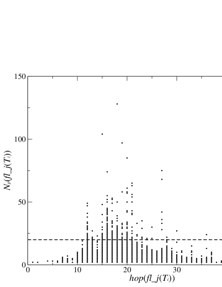
Figure 9: $hop\left(fl\_j\left(T_{i}\right)\right)$ vs. $N_{p}\left(fl\_j\left(T_{i}\right)\right)$ for the trace of Data I given in Fig. 1.

We investigated hop counts $hop\left(fl\_j\left(T_{i}\right)\right)$ of each per-time-unit flow $fl\_j\left(T_{i}\right)$ for all traces of Data I, using the hop count estimation methodology described above. Here, we removed flows having multiple hop counts for one source IP address. Figure 9 shows the relationship between $hop\left(fl\_j\left(T_{i}\right)\right)$ and $N_{p}\left(fl\_j\left(T_{i}\right)\right)$ for the trace given in Fig 1. Hop counts of greedy flows (above the dashed line) can be considered to be smaller than those of all flows. Figure 10 shows a histogram of $hop\left(fl\_j\left(T_{i}\right)\right)$ for (a) all per-time-unit flows and (b) for greedy per-time-unit flows, where we used all traces of Data I. Average hop counts for greedy flows were smaller than those of all flows, and most greedy flows had relatively smaller hop counts. Actually, average hop counts were 20.84 for all flows and 18.22 for greedy flows (see dashed lines in Fig. 10) .

From these results, we conclude that greedy flows had smaller hop counts than those of all flows in our study. This is because the RTTs of flows with smaller hop counts are assumed to be smaller statistically, as demonstrated in [2], and TCP flows with smaller RTTs can quickly make their window size larger (i.e., can become greedy) following the mechanism of TCP flow control. Accordingly we can assume that if TCP flows having smaller hop counts (i.e., smaller RTTs) exist with non-negligible probability, then the aggregated traffic shows a non-Gaussian nature. To verify the above assumptions, we examine the relationship between hop counts and RTT, and protocol distribution for our trace data in the following two sections. Our goal is to verify the linear relationship between hop counts and RTTs, and protocol breakdown for trace data used in this study.

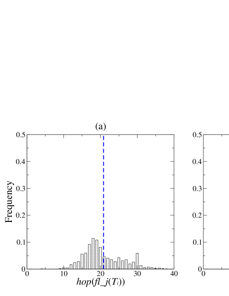
Figure 10: Histogram of $hop\left(fl\_j\left(T_{i}\right)\right)$ for all traces of Data I. (a) is for all per-time-unit flows and (b) is for greedy ones. The dashed lines indicate average hop counts.

3.5 Relationship between hop counts and RTTs

Here, we introduce the technique for estimating RTTs from given passively measured traces and then give results of analyses for our trace data. Our approach is based on the technique proposed in [2], which is to analyze TCP’s 3-way handshake packets. Adding to the description given in [2], we give a more detailed description of the technique. Figure 11 diagrams this between hosts $\alpha$ and $\beta$. For convenience, we call a TCP packet with a SYN (SYN and ACK, ACK) flag bit on a SYN (SYN+ACK, ACK) packet. In our study, we measured traffic at measuring point M between the two hosts.

First host $\alpha$ sends a SYN packet in order to request connection establishment. Let the time at this moment be $t_{\alpha}\left(S\right)$. The SYN packet passes the measuring point at $t_{M}\left(S\right)$, and is received by host $\beta$ at $t_{\beta}\left(S\right)$. Immediately upon receiving the SYN packet, host $\beta$ sends back a SYN+ACK packet at $t_{\beta}\left(SA\right)$, and it is received by host $\alpha$ at $t_{\alpha}\left(SA\right)$. Similarly, host $\alpha$ immediately sends back an ACK packet at $t_{\alpha}\left(A\right)$, and it passes measuring point M at $t_{M}\left(A\right)$, and it is received by host $\beta$ at $t_{\beta}\left(A\right)$ for the end of negotiation. Assuming that the delay caused by transactions of each host is quite small (i.e., $t_{\beta}\left(S\right)\sim t_{\beta}\left(SA\right),t_{\alpha}\left(SA\right)\sim t_{\alpha}\left(A\right)$) and there is no queueing delay caused by network congestion, RTT between host $\alpha$ and $\beta$ can be estimated as $t_{M}\left(A\right)-t_{M}\left(S\right)$ as described in the figure .

Using the above approach, we estimated RTTs of IP flows that contain TCP’s 3-way handshake, where we removed flows that contain duplicated SYN and SYN+ACK to estimate RTTs exactly. In the trace of Data I given in Fig. 1, the total number of IP flows in the Internet-to-ECL direction was 16,358. We could estimate RTTs for 6834 of them and estimate both RTTs and hop counts for 1987 of them.

Figure 11: Diagram of TCP’s 3-way handshake.

Figure 12 shows (a) the relationship between hop counts and number of IP flows and (b) the relationship between hop counts and the average of estimated RTTs, where we collected estimated RTTs per hop count and used their average as a representative value. The correlation coefficient of the average of the estimated RTTs and hop counts was 0.93, where the regression range of hop counts $h$ was set to $14\leq h\leq 30$, where the number of IP flows exceeds 1% (inside dashed lines). The result indicates that hop counts and RTTs are in good agreement with a linear correlation. Thus, it was verified that statistically, IP flows with smaller (larger) hop counts have smaller (larger) RTTs for trace data used in this study. This suggests that if the IP flow has smaller hop counts and its protocol is TCP, it can be greedier, following the mechanisms of TCP as mentioned in the previous paragraph. In the next section, we show the protocol distribution for trace data.

3.6 Protocol distribution

For each per-time-unit flow $fl\_j\left(T_{i}\right)$, we investigated the protocol. Table 4 shows the protocol distribution of all per-time-unit flows and greedy per-time-unit flows for Data I and II. The results show that for both cases, most of their protocols were TCP. That is, most per-time-unit flows followed TCP’s flow control mechanism, and if flows had smaller RTTs (i.e., smaller hop counts as shown in previous section), they could quickly make their window size larger and be greedy in a short time, leading to the non-Gaussian nature of aggregated network traffic. As today’s most popular Internet applications such as WWW are based on TCP (HTTP), this implication is very important.

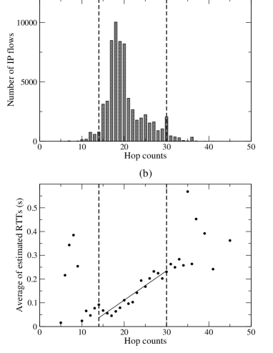
Figure 12: (a) Hop counts vs. number of IP flows and (b) hop counts vs. average of estimated RTTs.

4 Conclusion

In this work, we showed the performance implication of the non-Gaussian nature of network traffic and analyzed its mechanisms using some Internet traffic data. Our main findings are that (1) the non-Gaussian nature degrades network performance, (2) it is caused by greedy existing flows with non-negligible probability, and (3) a large majority of greedy flows are TCP flows having relatively small hop counts, which correspond to small RTTs. Accordingly, we conclude that in a network that has greedy flows with non-negligible probability, a traffic controlling scheme or bandwidth design that considers non-Gaussian nature is essential.

We expect that detecting non-Gaussian factors will allow us to propose practical methodologies for traffic engineering. We show some examples below. As we have shown in section 3, the behavior of each IP flow is related to its hop count; that is, IP flows with smaller hop counts tends to be greedier than ones with larger hop counts. So, classifying IP flows with their hop counts (e.g., using TTL fields) at routers will be useful for traffic engineering. For instance, decreasing queueing priority for IP flows with smaller hop counts will decrease the number of possible greedy flows. The decrease in the number of greedy flows will let the nature of aggregated traffic to be close to Gaussian, where network performance will be improved for a given utilization and buffer capacity, as we showed in Fig. 4. It will also lead to the establishment of fairness among IP flows. Another example is to clarify the relationship between traffic characterization and network topology as mentioned in section 3. Efficient network design according to its topology will be established by this study. That is, from the hop count distribution obtained by analyzing the network topology, we can estimate whether the network is likely to have greedy flows (i.e., IP flows having smaller hop counts). If it does with non-negligible probability, then the aggregated traffic will show non-Gaussian nature and bandwidth design considering the effect of non-Gaussian nature will be effective for efficient operation of the network.

Table 4: Protocol distribution for all per-time-unit flows and greedy ones.

	Data I		Data II
	All	Greedy	All	Greedy
TCP	97.00 %	99.90 %	95.76 %	95.36 %
UDP	1.02 %	0.10 %	4.20 %	4.62 %
Other	1.98 %	0.00 %	0.04 %	0.01 %

We consider that the existence of greedy flows is due to the heterogeneity of the Internet. As shown in section 3.2, flows were aggregated in various manners on a certain time scale. Actually, they were following a power-law (Fig. 6). We expect that this power-law mainly comes from (a) the heterogeneity of network topology, which is partly found in hop count distributions or (b) the heterogeneity of user links, which ranges from low-speed links such as analog modem to high-speed links such as gigabit Ethernet. So, in the Internet, there exist various kinds of IP flows and this diversity leads to greedy flows existing with non-negligible probability. As pointed out in [10], learning the characteristics of the Internet is an immensely challenging undertaking because of the network’s great heterogeneity and rapid changes. However, we believe that seeking some invariant characteristics in the Internet such as self-similarity or non-Gaussian nature or power-law of per-time-unit flows will help us to build practical models of it and propose methodologies for operating it efficiently.

References

- [1] J. Beran, Statistics for long-memory processes. Chapman & Hall, New York, 1994.
- [2] K. Fujii and S. Goto, “Correlation between hop count and packet transfer time”, APAN/IWS2000, February 2000.
- [3] M. Grossglauser and J. C. Bolot, “On the relevance of long-range dependence in network traffic”, IEEE/ACM Transactions on Networking, pp. 629-640, October 1999.
- [4] Postel, J., Editor, “Transmission control protocol”, STD 7, RFC 793, September 1981.
- [5] R. Kawahara, K. Ishibashi, T. Hirano, H. Saito, H. Ohara, D. Satoh, S. Asano and J. Matsukata, “Traffic measurement and analysis in an ATM-based internet backbone”, Computer Communications, Vol. 24, pp. 1508-1524, 2001.
- [6] W. E. Leland, M. S. Taqqu, W. Willinger, and D. V. Wilson, “On the self-similar nature of ethernet traffic” (Extended Version), IEEE/ACM Transactions on Networking, Vol. 2, No. 1, Feb 1994.
- [7] I. Norros, “On the use of fractional brownian motion in the theory of connectionless networks, IEEE Journal on Selected Areas in Communications”, Vol. 13, No. 6, August 1995.
- [8] K. Park, G. Kim, and M. Crovella. “On the effect of traffic self-similarity on network performance”, In Proc. of the SPIE International Conference on Performance and Control of Network Systems, November, 1997.
- [9] K. Park and W. Willinger, Self-similar network traffic and performance evaluation, Wiley Interscience, 2000.
- [10] V. Paxson, and S. Floyd, “Why we don’t know how to simulate the internet”, Proceedings of the 1997 Winter Simulation Conference, December 1997.
-
[11]
L. Spitzner, “Know your enemy: passive fingerprinting”,
http://project.honeynet.org/papers/finger/,
March 2002. - [12] M. S. Taqqu, V. Teverovsky and W. Willinger, “Estimators for long-range dependence: an empirical study”, Fractals, Vol. 3, No. 4, 785-788, 1995.
-
[13]
The internet traffic archive
http://ita.ee.lbl.gov/index.html -
[14]
The network simulator - ns-2,
http://isi.edu/nsnam/ns/ - [15] K. Thompson, G. Miller, and R. Wilder, “Wide area internet traffic patterns and characteristics”, IEEE Network, November 1997
- [16] W. Willinger and M. S. Taqqu, “Self-similarity through high variability: statistical analysis of ethernet LAN traffic at the source level”, IEEE/ACM Transactions on Networking, February 1997.