Abstract

The advent of multicast and the growth and complexity of the Internet has complicated network protocol design and evaluation. Evaluation of Internet protocols usually uses random scenarios or scenarios based on designers’ intuition. Such approach may be useful for average-case analysis but does not cover boundary-point (worst or best-case) scenarios. To synthesize boundary-point scenarios a more systematic approach is needed.

In this paper, we present a method for automatic synthesis of worst and best case scenarios for protocol boundary-point evaluation. Our method uses a fault-oriented test generation (FOTG) algorithm for searching the protocol and system state space to synthesize these scenarios. The algorithm is based on a global finite state machine (FSM) model. We extend the algorithm with timing semantics to handle end-to-end delays and address performance criteria. We introduce the notion of a virtual LAN to represent delays of the underlying multicast distribution tree. The algorithms used in our method utilize implicit backward search using branch and bound techniques and start from given target events. This aims to reduce the search complexity drastically.

As a case study, we use our method to evaluate variants of the timer suppression mechanism, used in various multicast protocols, with respect to two performance criteria: overhead of response messages and response time. Simulation results for reliable multicast protocols show that our method provides a scalable way for synthesizing worst-case scenarios automatically. Results obtained using stress scenarios differ dramatically from those obtained through average-case analyses. We hope for our method to serve as a model for applying systematic scenario generation to other multicast protocols.

1 Introduction

The longevity and power of Internet technologies derives from its ability to operate under a wide range of operating conditions (underlying topologies and transmission characteristics, as well as heterogeneous applications generating varied traffic inputs). Perhaps more than any other technology, the range of operating conditions is enormous (it is the cross product of the top and bottom of the IP protocol stack).

Perhaps it is this enormous set of conditions that has inhibited the development of systematic approaches to analyzing Internet protocol designs. How can we test correctness or characterize performance of a protocol when the set of inputs is intractable? Nevertheless, networking infrastructure is increasingly critical and there is enormous need to increase the understanding and robustness of network protocols. Most current approaches for protocol evaluation use average-case analysis and are based on random or intuitive scenarios. Such approach does not address protocol robustness or boundary-point analysis, in which the protocol exhibits worst or best-case behavior. We believe that such protocol breaking points should be identified and studied in depth to understand and hopefully increase protocol robustness. It is time to develop techniques for systematic testing of protocol behavior, even in the face of the above challenges and obstacles. At the same time we do not expect that complex adaptive protocols will be automatically verifiable under their full range of conditions. Rather, we are proposing a framework in which a protocol designer can follow a set of systematic steps, assisted by automation where possible, to cover a specific part of the design and operating space. Our goal is to complement average case studies and enrich the evaluation test-suites for multicast protocols.

In our proposed framework, a protocol designer will still need to create the initial mechanisms, describe it in the form of a finite state machine, and identify the performance criteria or correctness conditions that need to be investigated. Our automated method will pick up at that point, providing algorithms that generate scenarios or test suites that stress the protocol with respect to the identified criteria. The algorithms used in our method utilize implicit backward search using branch and bound techniques and start from given target events. This aims to reduce the search complexity drastically, as we shall discuss based on our case studies.

This paper demonstrates our progress in realizing this vision as we present our method and apply it to boundary-point (worst and best-case) performance evaluation of the timer suppression mechanism used in numerous multicast protocols.

1.1 Motivation

The recent growth of the Internet and its increased heterogeneity has introduced new failure modes and added complexity to protocol design and testing. In addition, the advent of multicast applications has introduced new challenges of qualitatively different nature than the traditional point-to-point protocols. Multicast applications involve a group of receivers and one or more senders. As more complex multicast applications and protocols are coming to life, the need for systematic and automatic methods to study and evaluate such protocols is becoming more apparent. Such methods aim to expedite the protocol development cycle and improve resulting protocol robustness and performance.

Through our proposed methodology for test synthesis, we hope to address the following key issues of protocol design and evaluation.

• Scenario dependent evaluation, and the use of validation test suites: Protocols may be evaluated for correctness and performance. In many evaluation studies of multicast protocols, the results are dependent upon several factors, such as membership distribution and network topology, among others. Hence, conclusions drawn from these studies depend heavily upon the evaluation scenarios.

  Protocol development usually passes through iterative cycles of refinement, which requires revisiting the evaluation scenarios to ensure that no erroneous behavior has been introduced. This brings about the need for validation test suites. Constructing these test suites can be an onerous and error-prone task if performed manually. Unfortunately, little work has been done to automate the generation of such tests for multicast network protocols. In this paper, we propose a method for synthesizing test scenarios automatically for boundary-point analysis of timer-suppression mechanisms employed by several classes of Internet multicast protocols.

• Worst-case analysis of protocols: It is difficult to design a protocol that would perform well in all environments. However, identifying breaking points that violate correctness or exhibit worst-case performance behaviors of a protocol may give insight to protocol designers and help in evaluating design trade-offs. In general, it is desirable to identify, early on in the protocol development cycle, scenarios under which the protocol exhibits worst or best case behavior. The method presented in this paper automates the generation of scenarios in which multicast protocols exhibit worst and best case behaviors.

• Performance benchmarking: New protocols may propose to refine a mechanism with respect to a particular performance metric, using for evaluation those scenarios that show performance improvement. However, without systematic evaluation, these refinement studies often (though unintentionally) overlook other scenarios that may be relevant. To alleviate such a problem we propose to integrate stress test scenarios that provide an objective benchmark for performance evaluation.

  Using our scenario synthesis methodology we hope to contribute to the understanding of better performance benchmarking and the design of more robust protocols.

1.2 Background

The design of multicast protocols has introduced new challenges and problems. Some of the problems are common to a wide range of protocols and applications. One such problem is the multi-responder problem, where multiple members of a group may respond (almost) simultaneously to an event, which may cause a flood of messages throughout the network, and in turn may lead to synchronized responses, and may cause additional overhead (e.g., the well-known Ack implosion problem), leading to performance degradation.

One common technique to alleviate the above problem is the multicast damping technique, which employs a timer suppression mechanism (TSM). TSM is employed in several multicast protocols, including the following:

• IP-multicast protocols, e.g., PIM [1] [2] and IGMP [3], use TSM on LANs to reduce Join/Prune control overhead.

• Reliable multicast schemes, e.g., SRM [4] and MFTP [5], use this mechanism to alleviate Ack implosion. Variants of the SRM timers are used in registry replication (e.g., RRM [6] [7]) and adaptive web caching [8].

• Multicast address allocation schemes, e.g., AAP and SDr [9], use TSM to avoid an implosion of responses during the collision detection phase.

• Active services [10] use multicast damping to launch one service agent ‘servent’ from a pool of servers.

TSM is also used in self-organizing hierarchies (SCAN [11]), and transport protocols (e.g., XTP [12] and RTP [13]).

We believe TSM is a good building block to analyze as our first end-to-end case study, since it is rich in multicast and timing semantics, and can be evaluated using standard performance criteria. As a case study, we examine its worst and best case behaviors in a systematic, automatic fashion.

In TSM, a member of a multicast group that has detected loss of a data packet multicasts a request for recovery. Other members of the group, that receive this request and that have previously received the data packet, schedule transmission of a response. In general, randomized timers are used in scheduling the response. While a response timer is running at one node, if a response is received from another node then the response timer is suppressed to reduce the number of responses triggered. Consequently, the response time may be delayed to allow for more suppression.

Two main performance evaluation criteria used in this case are overhead of response messages and time to recover from packet loss. Depending on the relative delays between group members and the timer settings, the mechanism may exhibit different performance. In this study, our method attempts to obtain scenarios of best case and worst case performance according to the above criteria.

We are not aware of any related work that attempts to achieve this goal systematically. However, we borrow from previous work on protocol verification and test generation.

The rest of the paper is organized as follows. Section 2 introduces the protocol and topology models. Section 3 outlines the main algorithm, and Section 4 presents the model for TSM. Sections 5 and  6 present performance analyses for protocol overhead and response time, and Section 7 presents simulation results. Related work is described in Section 8. Issues and future work are discussed in Section 9. We present concluding remarks in Section 10. Algorithmic details, mathematical models and example case studies are given in the appendices.

2 The Model

The model is a processable representation of the system under study that enables automation of our method. Our overall model consists of: A) the protocol model, B) the topology model, and C) the fault model.

2.1 The Protocol Model

We represent the protocol by a finite state machine (FSM) and the overall system by a global FSM (GFSM).

I. FSM model: Every instance of the protocol, running on a single end-system, is modeled by a deterministic FSM consisting of: (i) a set of states, (ii) a set of stimuli causing state transitions, and (iii) a state transition function (or table) describing the state transition rules. A protocol running on an end-system $i$ is represented by the machine ${\mathcal{M}}_{i}=({\mathcal{S}}_{i},\tau_{i},\delta_{i})$, where ${\mathcal{S}}_{i}$ is a finite set of state symbols, $\tau_{i}$ is the set of stimuli, and $\delta_{i}$ is the state transition function ${\mathcal{S}}_{i}\times\tau_{i}\rightarrow{\mathcal{S}}_{i}$.

II. Global FSM model: The global state is defined as the composition of individual end-system states. The behavior of a system with $n$ end-systems may be described by $\mathcal{M}_{\mathcal{G}}=(\mathcal{S}_{\mathcal{G}},\tau_{\mathcal{G}},\delta_{\mathcal{G}})$, where $\mathcal{S}_{\mathcal{G}}$: ${\mathcal{S}}_{1}\times{\mathcal{S}}_{2}\times\dots\times{\mathcal{S}}_{n}$ is the global state space, $\tau_{\mathcal{G}}$: $\overset{n}{\underset{i=1}{\bigcup}}\tau_{i}$ is the set of stimuli, and $\delta_{\mathcal{G}}$ is the global state transition function $\mathcal{S}_{\mathcal{G}}\times\tau_{\mathcal{G}}\rightarrow\mathcal{S}_{\mathcal{G}}$.

2.2 The Topology Model

The topology cannot be captured simply by one metric. Indeed, its dynamics may be complex to model and sometimes intractable. We model the topology at the network layer and we abstract the network using end-to-end delays. We model the delays using the delay matrix and loss patterns using the fault model. We use a virtual LAN (VLAN) model to represent the underlying network topology and multicast distribution tree. The VLAN captures delay semantics using a delay matrix $D$ (see Figure 1), where $d_{i,j}$ is the delay from system $i$ to system $j$. The VLAN model may seem as an over-simplification of the topology as it abstracts the internal network connectivity and queues. This, however, renders our model tractable and is quite useful in obtaining characteristics of boundary-point scenarios. We shall further investigate the utility and accuracy of our model in Section 7 through detailed packet level simulations of sophisticated timer mechanisms over complex topologies.

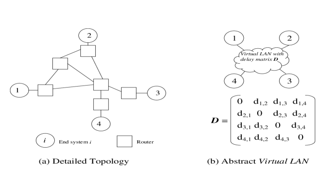
Figure 1: Representing network details using virtual LAN and delay matrix D. ($d_{i,j}$ is delay from $i$ to $j$.)

2.3 The Fault Model

A fault is a low level (e.g., physical layer) anomalous behavior that may affect the protocol under test. Faults may include packet loss, system crashes, or routing loops. For brevity, we only consider selective packet loss in this study. Selective packet loss occurs when a multicast message is received by some group members but not others. The selective loss of a message prevents the transition that this message triggers at the intended recipient.

3 Algorithm and Objectives

To apply our method, the designer specifies the protocol as a global FSM model. In addition, the evaluation criteria, be it related to performance or correctness, are given as input to the method. In this paper we address performance criteria, correctness has been addressed in previous studies [14, 15]. The algorithm operates on the specified model and synthesizes a set of ‘test scenarios’; protocol events and relations between topology delays and timer values, that stress the protocol according to the evaluation criteria (e.g., exhibit maximum overhead or delay). In this section, we outline the algorithmic details of our method. The algorithm is further discussed in Section 5 and illustrated by a case study. Algorithmic complexity issues are discussed in Section 9.

3.1 Algorithm Outline

Our algorithm is a variant of the fault-oriented test generation (FOTG) algorithm presented in [15]. It includes the topology synthesis, the backward search and the forward search stages. Here we describe those aspects of our algorithm that deal with timing and performance semantics. The basic algorithm passes through three main steps (1) the target event identification, (2) the search, and (3) the task specific solution. The algorithm is outlined in Figure 2.

1. The target event: The algorithm starts from a given event, called the ‘target event’. The target event (e.g., sending a message) is identified by the designer based on the protocol evaluation criteria, e.g., overhead.

2. The search: Three steps are taken in the search: (a) identifying conditions, (b) obtaining sequences, and (c) formulating inequalities.

   1. Identifying conditions: The algorithm uses the protocol transition rules to identify transitions necessary to trigger the target event and those that prevent it, these transitions are called wanted transitions and unwanted transitions, respectively.

   2. Obtaining sequences: Once the above transitions are identified, the algorithm uses backward and forward search to build event sequences leading to these transitions and calculates the times of these events as follows.

      1. Backward search is used to identify events preceding the wanted and unwanted transitions, and uses implication rules that operate on the protocol’s transition table. Section 4.2.5 describes the implication rules.

      2. Forward search is used to verify the backward search. Every backward step must correspond to valid forward step(s). Branches leading to contradictions between forward and backward search are rejected. Forward search is also used to complete event sequences necessary to maintain system consistency.

   3. Formulating inequalities: Based on the transitions and timed sequences obtained in the previous steps, the algorithm formulates relations between timer values and network delays that trigger the wanted transitions and avoid the unwanted transitions.

3. Task specific solution: The output of the search is a set of event sequences and inequalities that satisfy the evaluation criteria. These inequalities are solved mathematically to find a topology or timer configuration, depending on the task definition.

3.2 Task Definition

We apply our method to two kinds of tasks:

1. Topology synthesis is performed to identify the delays, $d_{i,j}$, in the dealy matrix $D$ that produce the best or worst case behavior, given the timer values.

2. Timer configuration is performed to obtain the timer values that cause the best and worst case behavior, given the topology delay matrix $D$.

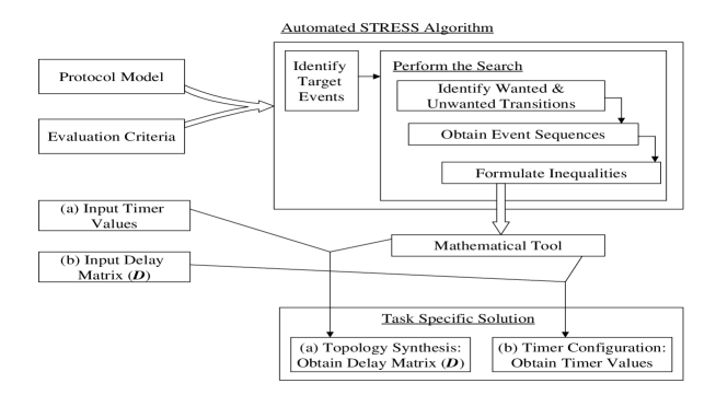
Figure 2: STRESS framework for boundary-point scenario synthesis.

4 The Timer Suppression Mechanism (TSM)

In this section, we present a simple description of TSM, then present its model, used thereafter in the analysis. TSM involves a request, $q$, and one or more responses, $p$. When a system, $Q$, detects the loss of a data packet it sets a request timer and multicasts a request $q$. When a system $i$ receives $q$ it sets a response timer (e.g., randomly), the expiration of which, after duration $Exp_{i}$, triggers a response $p$. If the system $i$ receives a response $p$ from another system $j$ while its timer is running, it suppresses its own response.

4.1 Performance Evaluation Criteria

We use two performance criteria to evaluate TSM:

1. Overhead of response messages, where the worst case produces the maximum number of responses per data packet loss. As an extreme case, this occurs when all potential responders respond and no suppression takes place.

2. The response delay, where worst case scenario produces maximum loss recovery time.

4.2 Timer Suppression Model

Following is the TSM model used in the analysis.

4.2.1 Protocol states ($\mathcal{S}$)

Following is the state symbol table for the TSM model.

State	Meaning
$R$	original state of the requester $Q$
$R_{T}$	requester with the request timer set
$D$	potential responder
$D_{T}$	responder with the response timer set

4.2.2 Stimuli or events

1. Sending/receiving messages: transmitting response ($p_{t}$) and request ($q_{t}$), receiving response ($p_{r}$) and request ($q_{r}$).

2. Timer events and other events: the events of firing the request timer, $Req$, and response timer, $Res$, and the event of detecting packet loss, $L$.

4.2.3 Notation

Following are the notations used in the transition table and the analysis thereafter.

• An event subscript denotes the system initiating the event, e.g., $p_{t_{i}}$ is response sent by system $i$, while the subscript $m$ denotes multicast reception, e.g., $p_{r_{m}}$ denotes scheduled reception of a response by all members of the group if no loss occurs. When system $i$ receives a message sent by system $j$, this is denoted by the subscript $i,j$, e.g., $p_{r_{i,j}}$ denotes system $i$ receiving response from system $j$.

• The state subscript $T$ denotes the existence of a timer, and is used by the algorithm to apply the timer implication to fire the timer event after the expiration period $Exp$.

• A state transition has a $start$ state and an $end$ state and is expressed in the form $startState\rightarrow endState$ (e.g. $D\rightarrow D_{T}$). It implies the existence of a system in the $startState$ (i.e., $D$) as a condition for the transition to the $endState$ (i.e., $D_{T}$).

• Effect in the transition table may contain transition and stimulus in the form ($startState\rightarrow endState).stimulus$, which indicates that the condition for triggering $stimulus$ is the state transition. An effect may contain several transitions (e.g., $Trans1$, $Trans2$), which means that out of these transitions only those with satisfied conditions will take effect.

• To describe event sequences in the backward search we denote $a\Leftarrow b$, where $a$ and $b$ are global states, which means that $a$ succeeds $b$ in the event sequence, and that $b$ can be implied from $a$. Also, for forward search we use $a\Rightarrow b$, which means that $a$ precedes $b$ in the event sequence and that $b$ can be implied from $a$.

4.2.4 Transition table

Following is the transition table for TSM.

Symbol	Event	Effect	Meaning
$loss$	$L$	$(R\rightarrow R_{T}).q_{t}$	Loss detection causes $q_{t}$ and setting of request timer
$tx\_req$	$q_{t}$	$q_{r_{m}}$	Transmission of $q$ causes multicast reception of $q$ after network delay
$rcv\_req$	$q_{r}$	$D\rightarrow D_{T}$	Reception of $q$ causes a system in $D$ state to set response timer
$res\_tmr$	$Res$	$(D_{T}\rightarrow D).p_{t}$	Response timer expiration causes transmission of $p$ and a change to $D$ state
$tx\_res$	$p_{t}$	$p_{r_{m}}$	Transmission of $p$ causes multicast reception of $p$ after network delay
$rcv\_res$	$p_{r}$	$R_{T}\rightarrow R$, $D_{T}\rightarrow D$	Reception of $p$ by a system with the timer set causes suppression
$req\_tmr$	$Req$	$q_{t}$	Expiration of request timer causes re-transmission of $q$

The model contains a requester, $Q$, and several potential responders (e.g., $i$ and $j$). Initially, the requester, $Q$, exists in state $R$ and all potential responders exist in state $D$. Let $t_{0}$ be the time at which $Q$ sends the request, $q$. The request sent by $Q$ is received by $i$ and $j$ at times $d_{Q,i}$ and $d_{Q,j}$, respectively. When the request, $q$, is sent, the requester transitions into state $R_{T}$ by setting the request timer. Upon receiving a request, a potential responder in state $D$ transitions into state $D_{T}$, by setting the response timer. The time at which an event occurs is given by $t(event)$, e.g., $q_{r_{j}}$ occurs at $t(q_{r_{j}})$.

4.2.5 Implication rules

The backward search uses the following cause-effect implication rules:

1. Transmission/Reception (Tx_Rcv): By the reception of a message, the algorithm implies the transmission of that message –without loss– sometime in the past (after applying the network delays). An example of this implication is $p_{r_{i,j}}\Leftarrow p_{t_{j}}$, where $t(p_{r_{i,j}})=t(p_{t_{j}})+d_{j,i}$.

2. Timer Expiration (Tmr_Exp): When a timer expires, the algorithm infers that it was set $Exp$ time units in the past, and that no event occurred during that period to reset the timer. An example of this implication is $Res_{i}.(D_{i}\leftarrow D_{T_{i}})\Leftarrow D_{T_{i}}$, where $t(Res_{i})=t(D_{T_{i}})+Exp_{i}$, and $Exp_{i}$ is the duration of the response timer $Res_{i}$.

3. State Creation (St_Cr): To build a history of events leading to a certain state, we reverse the transition rules and get to the $startState$ of the transitions leading to the creation of the state in question. For example, $D_{T_{i}}\Leftarrow(D_{T_{i}}\leftarrow D_{i})$ means that for the system to be in state $D_{T_{i}}$ the system must have existed in state $D_{i}$ and this is implied from the transition $(D_{T_{i}}\leftarrow D_{i})$.

In the following sections we use the above model to synthesize worst and best case scenarios according to protocol overhead and response time.

5 Protocol Overhead Analysis

In this section, we conduct worst and best case performance analyses for TSM with respect to the number of responses triggered per packet loss. Initially, we assume no loss of request or response messages until recovery, and that the request timer is high enough that the recovery will occur within one request round. The case of multiple request rounds is discussed in Appendix C.

5.1 Worst-Case Analysis

Worst-case analysis aims to obtain scenarios with maximum number of responses per data loss. In this section we present the algorithm to obtain inequalities that lead to worst-case scenarios. These inequalities are a function of network delays and timer expiration values.

5.1.1 Target event

Since the overhead in this case is measured as the number of response messages, the designer identifies the event of triggering a response, $p_{t}$, as the target event, and the goal is to maximize the number of response messages.

5.1.2 The search

As previously described in Section 3.1, the main steps of the search algorithm are to: (1) identify the wanted and unwanted transitions, (2) obtain sequences leading to the above transitions, and calculating the times for these sequences, and (3) formulate the inequalities that achieve the time constraints required to invoke wanted transitions and avoid unwanted transitions.

• Identifying conditions: The algorithm searches for the transitions necessary to trigger the target event, and their conditions, recursively. These are called wanted transitions and wanted conditions, respectively. The algorithm also searches for transitions that nullify the target event or invalidate any of its conditions. These are called unwanted transitions.

  In our case the target event is the transmission of a response (i.e., $p_{t}$). From the transition table described in Section 4.2.4, the algorithm identifies transition res_tmr, or $Res.(D_{T}\rightarrow D).p_{t}$, as a wanted transition and its condition $D_{T}$ as a wanted condition. Transition rcv_req, or $q_{r}.(D\rightarrow D_{T})$, is also identified as a wanted transition since it is necessary to create $D_{T}$. The unwanted transition is identified as transition rcv_res, or $p_{r}.(D_{T}\rightarrow D)$, since it alters the $D_{T}$ state without invoking $p_{t}$.

• Obtaining sequences: Using backward search, the algorithm obtains sequences and calculates time values for the following transitions: (1) wanted transition, res_tmr, (2) wanted transition rcv_req, and (3) unwanted transition rcv_res, as follows:

  1. To obtain the sequence of events for transition res_tmr, the algorithm applies implication rules (see Section 4.2.5) Tmr_Exp, St_Cr, Tx_Rcv in that order, and we get $res\_tmr_{i}\Leftarrow rcv\_req_{i}\Leftarrow tx\_req$, or

     $Res_{i}.(D_{i}\leftarrow D_{T_{i}}).p_{t_{i}}\Leftarrow q_{r_{i}}.(D_{T_{i}}\leftarrow D_{i})\Leftarrow q_{t}$.

     Hence the calculated time for $t(p_{t_{i}})$ becomes

     $$t(p_{t_{i}})=t_{0}+d_{Q,i}+Exp_{i},$$

     where $t_{0}$ is the time at which $q_{t}$ occurs.

  2. To obtain the sequence of events for transition rcv_req the algorithm applies implication rule Tx_Rcv, and we get $rcv\_req_{i}\Leftarrow tx\_req$, or

     $q_{r_{i}}.(D_{T_{i}}\leftarrow D_{i})\Leftarrow q_{t}$.

     Hence the calculated time for $t(q_{r_{i}})$ becomes

     $$t(q_{r_{i}})=t_{0}+d_{Q,i}.$$

  3. To obtain sequence of events for transition rcv_res for systems $i$ and $j$ the algorithm applies implication rules Tx_Rcv,Tmr_Exp, St_Cr, Tx_Rcv in that order, and we get $rcv\_res_{i}\Leftarrow res\_tmr_{j}\Leftarrow rcv\_req_{j}\Leftarrow tx\_req$, or

     $p_{r_{i,j}}.(D_{i}\leftarrow D_{T_{i}})\Leftarrow Res_{j}.(D_{j}\leftarrow D_{T_{j}}).p_{t_{j}}\Leftarrow q_{r_{j}}.(D_{T_{j}}\leftarrow D_{j})\Leftarrow q_{t}$.

     Hence the calculated time for $t(p_{r_{i,j}})$ becomes

     $$t(p_{r_{i,j}})=t_{0}+d_{Q,j}+Exp_{j}+d_{j,i}.$$

• Formulating Inequalities: Based on the above wanted and unwanted transitions the algorithm forms constraints and conditions to aoivd the unwanted transition, rcv_res, while invoking the wanted transition, res_tmr, to transit out of $D_{T}$. To achieve this, the algorithm automatically derives the following inequality (see Appendix A for more details):

  $$t(p_{t_{i}})<t(p_{r_{i,j}}).$$ (1)

  Substituting expressions for $t(p_{t_{i}})$ and $t(p_{r_{i,j}})$ previously derived, we get:

  $d_{Q,i}+Exp_{i}<d_{Q,j}+Exp_{j}+d_{j,i}$.

  Alternatively, we can avoid the unwanted transition rcv_res if the system did not exist in $D_{T}$ when the response is received. Hence, the algorithm automatically derives the following inequality (see Appendix A for more details):

  $$t(p_{r_{i,j}})<t(q_{r_{i}}).$$ (2)

  Again, substituting expressions derived above, we get:

  $d_{Q,i}>d_{Q,j}+Exp_{j}+d_{j,i}$.

  Note that equations (1) and (2) are general for any number of responders, where $i$ and $j$ are any two responders in the system. Figure 3 (a) and (b) show equations (1) and (2), respectively.

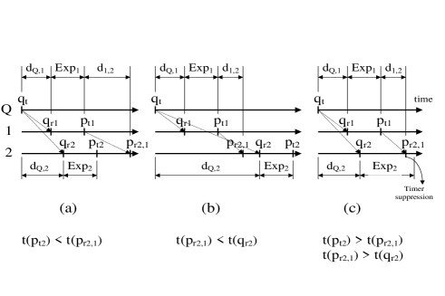
Figure 3: Event sequencing: sequences (a) & (b) do not lead to suppression, whereas (c) leads to suppression.

5.1.3 Task specific solutions

• Topology synthesis: Given the timer expiration values or ranges we want to find a feasible solution for the worst-case delays. A feasible solution in this context means assigning positive values to the delays $d_{i,j}\forall i,j$.

  In equation (1) above, if we take $d_{Q,i}=d_{Q,j}$, we get:

  $Exp_{i}-Exp_{j}<d_{j,i}$.

  These inequalities put a lower limit on the delays $d_{j,i}$, hence, we can always find a positive $d_{j,i}$ to satisfy the inequalities. Note that, the delays used in the delay matrix reflect delays over the multicast distribution tree. In general, these delays are affected by several factors including the multicast and unicast routing protocols, tree type and dynamics, propagation, transmission and queuing delays. One simple topology that reflects the delays of the delay matrix is a completely connected network where the underlying multicast distribution tree coincides with the unicast routing. There may also exist many other complex topologies that satisfy the delay matrix $D$.

• Timer configuration: Given the delay values, ranges or bounds, we want to obtain timer expiration values that produce worst-case behavior. We obtain a range for the relative timer settings (i.e., $Exp_{i}-Exp_{j}$) using equation (1) above.

The solution for the system of inequalities given by (1) and (2) above can be solved in the general case using linear programming (LP) techniques (see Appendix B for more details). Section 7 uses the above solutions to synthesize simulation scenarios.

Note, however, that it may not be feasible to satisfy all these constraints, due to upper bounds on the delays for example. In this case the problem becomes one of maximization, where the worst-case scenario is one that triggers maximum number of responses per packet loss. This problem is discussed in Appendix B.

5.2 Best-Case Analysis

Best case overhead analysis constructs constraints that lead to maximum suppression, i.e., minimum number of responses. The following conditions are formulated using steps similar to those given in the worst-case analysis:

$$t(p_{t_{i}})>t(p_{r_{i,j}}),$$ (3)

and

$$t(p_{r_{i,j}})>t(q_{r_{i}}).$$ (4)

These are complementary conditions to those given in the worst case analysis. Figure 3 (c) shows equations (3) and (4). Refer to the Appendix A for more details on the inequality derivation.

This concludes our description of the algorithmic details to construct worst and best-case delay-timer relations for overhead of response messages. Solutions to these relations represent delay and timer settings for stress scenarios that are used later on for simulations.

6 Response Time Analysis

In this section, we conduct the performance analysis with respect to response time, i.e., the time for the requester to recover from the packet loss. The algorithm obtains possible sequences leading to the target event and calculates the response time for each sequence. To synthesize the worst case scenario that maximizes the response time, for example, the sequence with maximum time is chosen.

To systematically approach this problem we consider the following three cases: (1) The case of no loss to the response message. This case leads to single round of request-response messages. Without loss of response messages this problem becomes one of maximizing the round trip delay between the requester and the first responder. (2) The case of single selective loss of the response message. This case may lead to two rounds of request-response messages. We analyze this case in the first part of this section. (3) The case of multiple selective losses of the response messages. This case may lead to more than two rounds of request-response messages, and is discussed at the end of this section.

We now consider the case of single selective loss of the response message during the recovery phase. For selective losses, transition rules are applied to only those systems that receive the message.

6.1 Target Event

The response time is the time taken by the mechanism to recover from the packet loss, i.e., until the requester receives the response $p$ and resets its request timer by transitioning out of the $R_{T}$ state. In other words, the response interval is $t(p_{r_{Q}})-t(q_{t})=t(p_{r_{Q}})-t_{0}$. The designer identifies $t(p_{r_{Q}})$ as the target time, hence, $p_{r_{Q}}$ is the target event.

6.2 The Search

We present in detail the case of single responder, then discuss the multiple responders case.

• Backward search: As shown in Figure 4 (a), the backward search starts from $p_{r_{Q}}$ and is performed over the transition table (see Section 4.2.4) using the implication rules in Section 4.2.5, yielding $rcv\_res_{Q}\Leftarrow res\_tmr_{j}\Leftarrow rcv\_req_{j}$, or :

  $D_{j}.p_{r_{Q}}.(R\leftarrow R_{T})\Leftarrow p_{t_{j}}.(D_{j}\leftarrow D_{T_{j}}).Res_{j}.R_{T}\Leftarrow q_{r_{j}}.(D_{T_{j}}\leftarrow D_{j}).R_{T}$

  At which point the algorithm reaches a branching point, where two possible preceding states could cause $q_{r_{j}}$:

  • The first is transition loss, or $D_{j}.q_{t}.(R_{T}\leftarrow R)$, and since the initial state $R$ is reached, the backward search ends for this branch.

  • The second is transition req_tmr, or $D_{j}.Req.q_{t}.R_{T}$. Note that $Req$ indicates the need for a transition to $R_{T}$, i.e., ($R_{T}\leftarrow R$), and the search for this last state yields the intial (data packet loss) state $loss$: $D_{j}.q_{t}.(R_{T}\leftarrow R)$. However, $q_{t}$ is message transmission, which implies that the message must be received (or lost). Hence, there are gaps in the event sequence (indicated by the $dots$ in Figure 4 (a)) that are filled through forward search (in Figure 4 (b)).

  

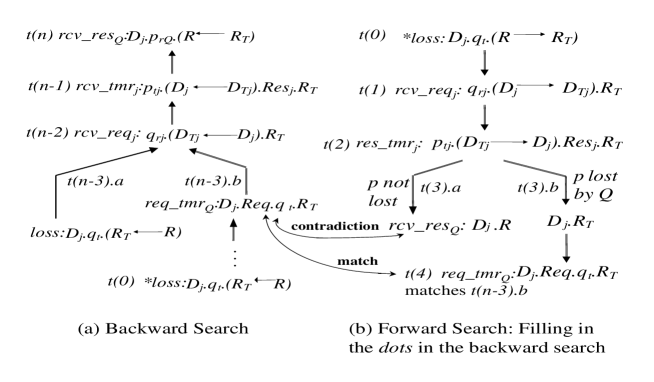
  Figure 4: Backward and forward search for response time analysis: (a) Backward search starts from the loss recovery state (at time $t(n)$) when the requester receives a response ($rcv\_res_{Q}$), and ends at the initial (packet $loss$) state at time $t(0)$. Part of the event sequence is incomplete (denoted by $dots$). (b) Forward search starts (at time $t(0)$) from the last state reached by the backward search after the $dots$ (denoted by $*loss$). It attempts to fill the gap in the sequence while checking for consistency, and finds a match.

• Forward search: The algorithm performs a forward search and checks for consistency of the GFSM. The forward search step may lead to contradiction with the original backward search, causing rejection of that branch as a feasible sequence. For example, as shown in Figure 4 (b), one possible forward sequence from the initial state gives $loss\Rightarrow tx\_req\Rightarrow rcv\_req_{j}\Rightarrow res\_tmr_{j}\Rightarrow tx\_res_{j}$, or:

  $D_{j}.q_{t}.(R\rightarrow R_{T})\Rightarrow q_{r_{j}}.(D_{j}\rightarrow D_{T_{j}}).R_{T}\Rightarrow p_{t_{j}}.(D_{T_{j}}\rightarrow D_{j}).Res_{j}.R_{T}$

  The algorithm then searches two possible next states:

  • If $p_{t_{j}}$ is not lost, and hence causes $p_{r_{Q}}$, then the next state is $D_{j}.R$. But the original backward search started from $D_{j}.q_{t}.Req.R_{T}$ which cannot be reached from $D_{j}.R$. Hence, we get contradiction and the algorithm rejects this sequence.

  • If the response $p$ is lost by $Q$, we get $D_{j}.R_{T}$ that leads to $D_{j}.Req.q_{t}.R_{T}$. The algorithm identifies this as a feasible sequence.

  Calculating the time for each feasible sequence, the algorithm identifies the latter sequence as one of maximum response time.

For multiple responders, the algorithm automatically explores the different possible selective loss patterns of the response message. The search identifies the sequence with maximum response as one in which only one responder triggers a response that is selectively lost by the requester. To construct such a sequence, the algorithm creates conditions and inequalities similar to those formulated for the best-case overhead analysis with respect to number of responses (see Section 5.2).

Effectively, the sequence obtained above occurs when the response is lost by the requester, which triggers another request. Intuitively, the response delay is increased with multiple request rounds. The case of multiple selective loss of the response messages may trigger multiple (more than two) request rounds. Practically, the number of request rounds is bounded by the protocol implementation, which imposes an upper bound on the number of requests sent per packet loss. This, in turn, imposes an upper bound on the worst-case response time. This bound can be easily integrated into the search to end the search when the maximum number of allowed request rounds is reached.

After conducting the above analyses, we have applied our method to generate worst-case overhead scenarios for topology synthesis and timer configuration tasks using determinsitic and adaptive timers (see Appendix D). We also applied it to response time analysis and to best-case analyses. In the next section we show network simulations using our generated worst-case overhead scenarios.

7 Simulations Using Systematic Scenarios

To evaluate the utility and accuracy of our method, we have conducted a set of detailed simulations for the Scalable Reliable Multicast (SRM) [4] based on our worst-case scenario synthesis results for the timer-suppression mechanism. We tied our method to the network simulator (NS) [16]. The output of our method, in the form of inequalities (see Section 5), is solved using a mathematical package (LINDO). The solution, in terms of a delay matrix, is then used to generate the simulation topologies for NS automatically.

For our simulations we measured the number of responses triggered for each data packet loss. We have conducted two sets of simulations, each using two sets of topologies. The simulated topologies included topologies with up to 200 receivers. The first set of topologies was generated according to the overhead analysis presented in this paper. We call this set of topologies the stress topologies. Example stress topology is shown in Figure 5 (a), and its corresponding fully-connected topology is shown in Figure 5 (b). Both topologies satisfy the delay matrix, $D$, produced by stress. The second set of topologies was generated by the GT-ITM topology generator [17], generating random and transit stub topologies. We call this set of topologies the random topologies.

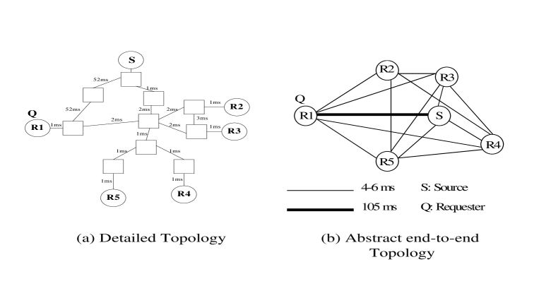
Figure 5: Example stress topology used for the simulation.

The first set of simulations was conducted for the SRM deterministic timers.The results of the simulation are shown in Figure 6 (a). The number of responses triggered for all the $stress$ topologies was $n-1$, where $n$ is the number of receivers (i.e., no suppression occurred). For the $random$ topologies, with up to 200 receivers, the number of responses triggered was less than 20 responses in the worst case.

Using the same two sets of topologies, the second set of simulations was conducted for the SRM adaptive timers. The results are given in Figure 6 (b). For the $stress$ topologies almost 50% of the receivers triggered responses. Whereas $random$ topologies simulation generated almost 10 responses in the worst case, for topologies with 100-200 receivers.

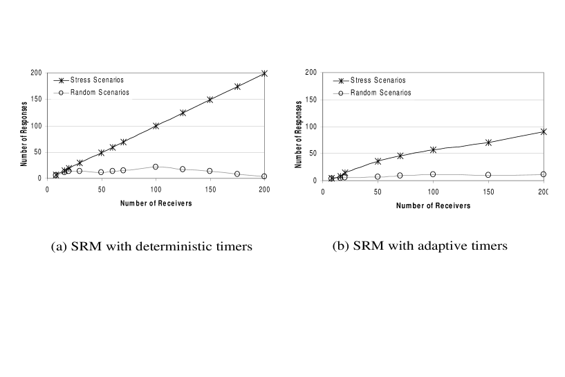
Figure 6: Simulation results for deterministic and adaptive timers over stress and random topologies.

These simulations illustrate how our method may be used to generate consistent worst-case scenarios in a scalable fashion. It is interesting to notice that worst-case topologies generated for simple deterministic timers also experienced substantial overhead (perhaps not the worst, though) for more complicated timers (such as the adaptive timers). It is also obvious from the simulations that stress scenarios are more consistent than the other scenarios when used to compare different mechanisms, in this case deterministic and adaptive timers; the performance gain for adaptive timers is very clear under stress scenarios.

So, in addition to experiencing the worst-case behavior of a mechanism, our stress methodology may be used to compare protocols in the above fashion and to aid in investigating design trade-offs. It is a useful tool for generating meaningful simulation scenarios that we believe should be considered in performance evaluation of protocols in addition to the average case performance and random simulations. We plan to apply our method to test a wider range of protocols through simulation.

8 Related Work

Related work falls mainly in the areas of protocol verification, VLSI test generation and network simulation.

There is a large body of literature dealing with verification of protocols. Verification systems typically address well-defined properties –such as safety, liveness, and responsiveness [24]– and aim to detect violations of these properties. In general, the two main approaches for protocol verification are theorem proving and reachability analysis [25]. Theorem proving systems define a set of axioms and relations to prove properties, and include model-based and logic-based formalisms [26, 27]. These systems are useful in many applications. However, these systems tend to abstract out some network dynamics that we study (e.g., selective packet loss). Moreover, they do not synthesize network topologies and do not address performance issues per se.

Reachability analysis algorithms [28], on the other hand, try to inspect reachable protocol states, and suffer from the ‘state space explosion’ problem. To circumvent this problem, state reduction techniques could be used [29]. These algorithms, however, do not synthesize network topologies. Reduced reachability analysis has been used in the verification of cache coherence protocols [30], using a global FSM model. We adopt a similar FSM model and extend it for our approach in this study. However, our approach differs in that we address end-to-end protocols, that encompass rich timing, delay, and loss semantics, and we address performance issues (such as overhead or response delays).

There is a good number of publications dealing with conformance testing [31] [32] [33] [34]. However, conformance testing verifies that an implementation (as a black box) adheres to a given specification of the protocol by constructing input/output sequences. Conformance testing is useful during the implementation testing phase –which we do not address in this paper– but does not address performance issues nor topology synthesis for design testing. By contrast, our method synthesizes test scenarios for protocol design, according to evaluation criteria.

Automatic test generation techniques have been used in several fields. VLSI chip testing [35] uses test vector generation to detect target faults. Test vectors may be generated based on circuit and fault models, using the fault-oriented technique, that utilizes implication techniques. These techniques were adopted in [15] to develop fault-oriented test generation (FOTG) for multicast routing. In [15], FOTG was used to study correctness of a multicast routing protocol on a LAN. We extend FOTG to study performance of end-to-end multicast mechanisms. We introduce the concept of a virtual LAN to represent the underlying network, integrate timing and delay semantics into our model and use performance criteria to drive our synthesis algorithm.

In [14], a simulation-based stress testing framework based on heuristics was proposed. However, that method does not provide automatic topology generation, nor does it address performance issues. The VINT [36] tools provide a framework for Internet protocols simulation. Based on the network simulator (NS) [16] and the network animator (NAM) [37], VINT provides a library of protocols and a set of validation test suites. However, it does not provide a generic tool for generating these tests automatically. Work in this paper is complementary to such studies, and may be integrated with network simulation tools similar to our work in Section 7.

9 Issues and Future Work

In this paper we have presented our first endeavor to automate the test synthesis as applies to boundary-point performance evaluation of multicast timer suppression protocols. Our case studies were by no means exhaustive. However, they gave us insights into the research issues involved. Particularly, in this section we shall discuss issues of algorithmic complexity. In addition, we present our future plans to explore several potential extensions and applications of our method.

• Algorithmic complexity

  One goal of our case studies is to understand and evaluate the computational complexity of our method and algorithms. Our main algorithm uses a mix of backward and forward search techniques. The algorithm starts from target events and uses implicit backward search and branch and bound techniques to synthesize the required scenario sequences. Complexity of such algorithm depends on the finite state machine (FSM), the state transition rules, and the target events from which the algorithm starts. Hence, it is hard to quantify, in general terms, the complexity of our algorithm. Nonetheless, we shall comment on the nature of the method and the algorithm qualitatively based on our case studies. We note the following: (a) Our algorithms use branch and bound techniques and utilize implicit backward search starting from a target event (vs. explicit forward reachability analysis starting from initial states). Branch and bound techniques are, generally, hard to quantify in terms of (worst-case or average case) complexity in abstract terms. Although the worst-case for branch and bound could be exponential, through our experiments we found that, on average, the target-based approach has far less complexity than forward search. In many cases the branch bounds immediately (e.g., due to contradiction if the sequence is not feasible). For all our STRESS case studies, we have found our search algorithms to be quite manageable. (b) Scenarios synthesized using the STRESS method usually are simple and include relatively small topologies. Thus, they often experience low computational complexity. It is our observation, in all our case studies thus far, that erroneous and worst-case protocol behaviors may be invoked using relatively simple (yet carefully synthesized) scenarios. Also, it was often the case that these simple scenarios were extensible to larger and more complex scenarios using simple heuristics. In Section 7, we have demonstrated how the simple scenarios generated by STRESS, with only a few receivers, could be scaled up to include hundreds of receivers. Accuracy of such extrapolation was validated through detailed simulations.

• Automated generation of simulation test suites

  Simulation is a valuable tool for designing and evaluating network protocols. Researchers usually use their insight and expertise to develop simulation inputs and test suites. Our method may be used to assist in automating the process of choosing simulation inputs and scenarios. The inputs to the simulation may include the topology, host events (such as traffic models), network dynamics (such as link failures or packet loss) and membership distribution and dynamics. Our future work includes implementing a more complete tool to automate our method (including search algorithms and modeling semantics) and tie it to a network simulator to be applied to a wider range of multicast protocols.

• Validating protocol building blocks

  The design of new protocols and applications often borrows from existing protocols or mechanisms. Hence, there is a good chance of re-using established mechanisms, as appropriate, in the protocol design process. Identifying, verifying and understanding building blocks for such mechanisms is necessary to increase their re-usability. Our method may be used as a tool to improve that understanding in a systematic and automatic manner. Ultimately, one may envision that a library of these building blocks will be available, from which protocols (or parts thereof) will be readily composable and verifiable using CAD tools; similar to the way circuit and chip design is carried out today using VLSI design tools. In this work and earlier works [15] [14], some mechanistic building blocks for multicast protocols were identified, namely, the timer-suppression mechanism and the Join/Prune mechanism (for multicast routing). More work is needed to identify more building blocks to cover a wider range of protocols and mechanisms.

• Generalization to performance bound analysis

  An approach similar to the one we have taken in this paper may be based on performance bounds, instead of worst or best case analyses. We call such approach ‘condition-oriented test generation’.

  For example, a target event may be defined as ‘the response time exceeding certain delay bounds’ (either absolute or parametrized bounds). If such a scenario is not feasible, that indicates that the protocol gives absolute guarantees (under the assumptions of the study). This may be used to design and analyze quality-of-service or real-time protocols, for example.

• Applicability to other problem domains

  So far, our method has been applied mainly to case studies on multicast protocols in the context of the Internet.

  Other problem and application domains may introduce new mechanistic semantics or assumptions about the system or environment. One example of such domains includes sensor networks. These networks, similar to ad-hoc networks, assume dynamic topologies, lossy channels, and deal with stringent power constraints, which differentiates their protocols from Internet protocols [38].

  Possible research directions in this respect include:

  • Extending the topology representation or model to capture dynamics, where delays vary with time.

  • Defining new evaluation criteria that apply to the specific problem domain, such as power usage.

  • Investigating the algorithms and search techniques that best fit the new model or evaluation criteria.

10 Conclusion

We have presented a methodology for scenario synthesis for boundary-point performance evaluation of multicast protocols. In this paper we applied our method to worst and best-case evaluation of the timer suppression mechanism; a common building block for various multicast protocols. We introduced a virtual LAN model to represent the underlying network topology and an extended global FSM model to represent the protocol mechanism. We adopted the fault-oriented test generation algorithm for search, and extended it to capture timing/delay semantics and performance issues for end-to-end multicast protocols.

Two performance criteria were used for evaluation of the worst and best case scenarios; the number of responses per packet loss, and the response delay. Simulation results illustrate how our method can be used in a scalable fashion to test and compare reliable multicast protocols.

We do not claim to have a generalized algorithm that applies to any arbitrary protocol. However, we hope that similar approaches may be used to identify and analyze other protocol building blocks. We believe that such systematic analysis tools will be essential in designing and testing protocols of the future.

Appendices: Algorithmic Details

In this appendix we present details of inequality formulation for the end-to-end performance evaluation. In addition, we present the mathematical model to solve these inequalities. We also discuss the case of multiple request rounds for the timer suppression mechanism, and present several example case studies.

Appendix A Deriving Stress Inequalities

Given the target event, transitions are identified as either wanted or unwanted transitions, according to the maximization or minimization objective. For maximization, wanted transitions are those that establish conditions to trigger the target event, while unwanted transitions are those that nullify these conditions.

Let $W$ be the wanted transition, and let $t(W)$ be the time of its occurrence. Let $C$ be the condition for the wanted transition, and let $t(C)$ be the time at which it is satisfied. Let $U$ be the unwanted transition occurring at $t(U)$.

We want to establish and maintain $C$ until $W$ occurs, i.e., in the duration [$t(C)$, $t(W)$]. Hence, $U$ may only occur outside (before or after) that interval. In Figure 7, this means that $U$ can only occur in $Region(1)$ or $Region(3)$.

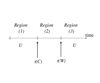
Figure 7: The time-line for transition ordering

Hence, the inequalities must satisfy the following

1. the condition for the wanted transition, $C$, must be established before the event for the wanted transition, $W$, triggers, i.e., $t(C)<t(W)$, and

2. one of the following two conditions must be satisfied:

   1. the unwanted transition, $U$, must occur before $C$, i.e., $t(U)<t(C)$, or

   2. the unwanted transition, $U$, must occur after the wanted transition, $W$, i.e., $t(W)<t(U)$.

These conditions must be satisfied for all systems. In addition, the algorithm needs to verify, using backward search and implication rules, that no contradiction exists between the above conditions and the nature of the events of the given protocol.

A.1 Worst-case Overhead Analysis

The target event for the overhead analysis is $p_{t}$. The objective for the worst case analysis is to maximize the number of responses $p_{t}$. The wanted transition is transition res_tmr, or $Res.(D_{T}\rightarrow D).p_{t}$ (see Section 4). Hence $t(W)=t(p_{t})$. The condition for the wanted transition is $D_{T}$ and its time is $t(C)=t(q_{r})$, from transition tx_req, or $q_{r}.(D\rightarrow D_{T})$.

The unwanted transition is one that nullifies the condition $D_{T}$. Transition rcv_res, or $p_{r}.(D_{T}\rightarrow D)$, is identified by the algorithm as the unwanted transition, hence $t(U)=t(p_{r})$.

For a given system $i$, the inequalities become:

$$t(q_{r_{i}})<t(p_{t_{i}}),$$

and either

$$t(p_{r_{i,j}})<t(q_{r_{i}})$$

or

$$t(p_{t_{i}})<t(p_{r_{i,j}}).$$

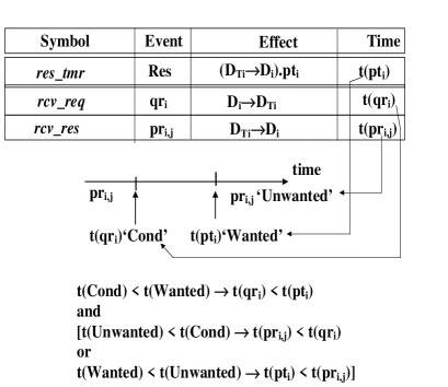
Figure 8: Formulating the inequalities automatically

The above automated process is shown in Figure 8. From the timer expiration implication rule, however, we get that the response time must have been set earlier by the request reception, i.e., $Res_{i}.(D_{i}\leftarrow D_{T_{i}}).p_{t_{i}}\Leftarrow q_{r_{i}}.(D_{T_{i}}\leftarrow D_{i})$ and $t(p_{t_{i}})=t(q_{r_{i}})+Exp_{i}$. Hence, $t(q_{r_{i}})<t(p_{t_{i}})$ is readily satisfied and we need not add any constraints on the expiration timers or delays to satisfy this condition. Thus, the inequalities formulated by the algorithm to produce worst-case behavior are:

$$t(p_{r_{i,j}})<t(q_{r_{i}}),$$

or

$$t(p_{t_{i}})<t(p_{r_{i,j}}).$$

A.2 Best-case Analysis

Using a similar approach to the above analysis, the algorithm identifies transition rcv_res, or $p_{r}.(D_{T}\rightarrow D)$, as the wanted transition. Hence $t(W)=t(p_{r})$, and $t(C)=t(q_{r})$. The unwanted transition is transition res_tmr, and $t(U)=t(p_{t})$.

For system $i$ the inequalities become:

$$t(q_{r_{i}})<t(p_{r_{i,j}}),$$

and either

$$t(p_{t_{i}})<t(q_{r_{i}})$$

or

$$t(p_{r_{i,j}})<t(p_{t_{i}}).$$

But from the backward implication we have $t(q_{r_{i}})<t(p_{t_{i}})$. Hence, the algorithm encounters contradiction and the inequality $t(p_{t_{i}})<t(q_{r_{i}})$ cannot be satisfied.

Thus, the inequalities formulated by the algorithm to produce best-case behavior are:

$$t(q_{r_{i}})<t(p_{r_{i,j}}),$$

and

$$t(p_{r_{i,j}})<t(p_{t_{i}}).$$

Appendix B Solving the System of Inequalities

In this section we present the general model of the constraints (or inequalities) generated by our method. As a first step, we form a linear programming problem and attempt to find a solution. If a solution is not found, then we form a mixed non-linear programming problem to get the maximum number of feasible constraints.

In general, the system of inequalities generated by our method to obtain worst or best case scenarios, can be formulated as a linear programming problem. In our case, satisfying all the constraints, regardless of the objective function, leads to obtaining the absolute worst/best case. For example, in the case of worst case overhead analysis, this means obtaining the scenario leading to no-suppression. The formulated inequalities by our method as given in Section 5 are as follows.

• for the worst case behavior:

  $$d_{Q,i}+Exp_{i}<d_{Q,j}+Exp_{j}+d_{j,i},$$

  or

  $$d_{Q,i}>d_{Q,j}+Exp_{j}+d_{j,i}.$$

• for the best case behavior:

  $$d_{Q,i}+Exp_{i}>d_{Q,j}+Exp_{j}+d_{j,i},$$

  and

  $$d_{Q,i}<d_{Q,j}+Exp_{j}+d_{j,i}.$$

The above systems of inequalities can be represented by a linear programming model. The general form of a linear programming (LP) problem is:

$$MaximizeZ=C^{T}X=\sum_{0\leq i\leq n}c_{i}\cdot x_{i}$$

subject to:

$$AX\leq B$$

$$X\geq 0$$

where $Z$ is the objective function (in our case it is a dummy objective function such as $Z=const$), $C$ is a vector of $n$ constants $c_{i}$, $X$ is a vector of $n$ variables $x_{i}$, $A$ is $m\times n$ matrix, and $B$ is a vector of $m$ elements. This problem can be solved practically in polynomial time using Karmarkar [39] or simplex method [40], if a feasible solution exists.

In some cases, however, the absolute worst/best case may not be attainable, and it may not be possible to find a feasible solution to the above problem. In such cases we want to obtain the maximum feasible set of constraints in order to get the worst/best case scenario. To achieve this, we define the problem as follows:

$$Maximize\sum_{0\leq i\leq m}y_{i}$$

subject to:

$$y_{i}\cdot f_{i}(x)\leq 0,\forall i$$

$$y_{i}\in\{0,1\}$$

or

$$y_{i}\cdot(1-y_{i})=0$$

where $f_{i}(x)$ is the original constraint from the previous problem.

This problem is a mixed integer non-linear programming (MINLP) problem, that can be solved using branch and bound methods [41].

Obtaining Link Delays:

In the previous discussion we assumed that the model deals only with end-to-end delays ($d_{i,j}$ of the delay matrix $D$). In some cases, however, it may be the case that the connectivity of the network topology is given and the task is to find the link delays (instead of end-to-end delays). We present a very simple extension to the model to accommodate such situation, as follows. Let $l_{x}$ be any link in the topology and let $d_{l_{x}}$ be its delay. Take any two end systems $i$ and $j$ and let the path from $i$ to $j$ pass through links $l_{a},l_{b},\dots\l_{n}$. Hence, we get $d_{i,j}=\sum_{x\in L}d_{l_{x}}$, where $L=\{l_{a},l_{b},\dots\l_{n}\}$. Substituting these relations in the above inequalities we can formulate the problem in terms of link delays.

Appendix C Multiple request rounds

In Section 5 we conducted the protocol overhead analysis with the assumption that recovery will occur in one round of request. In general, however, loss recovery may require multiple rounds of request, and we need to consider the request timer as well as the response timers. Considering multiple timers or stimuli adds to the branching factor of the search. Some of these branches may not satisfy the timing and delay constraints. It would be more efficient then to incorporate timing semantics into the search technique to prune off infeasible branches.

Let us consider forward search first. For example, consider the state $q_{t_{i}}.R_{T_{i}}$ having a transmitted request message and a request timer running. Depending on the timer expiration value $Exp_{i}$ and the delay experienced by the message $d_{i,j}$, we may get different successor states. If $d_{i,j}>Exp_{i}$ then the request timer fires first triggering the event $Req_{i}$ and we get $q_{t_{i}}.Req_{i}$ as the successor state. Otherwise, the request message will be received first, and the successor state will be $q_{r_{j}}.R_{T_{i}}$. Note that in this case the timer value must be decremented by $d_{i,j}$. This is illustrated in figure 9. The condition for branching is given on the arrow of the branch, and the timer value of $i$ is given by $T_{i}$.

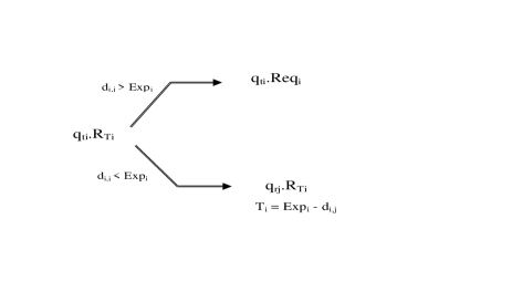
Figure 9: Forward search for multiple simultaneous events

For backward search, instead of decreasing timer values (as is done with forward search), timer values are increased, and the starting point of the search is arbitrary in time, as opposed to time ‘0’ for forward search.

To illustrate, consider the state having $(D_{i}\leftarrow D_{T_{i}}).R_{T_{j}}$, with the request timer running at $j$ and the response timer firing at $i$.

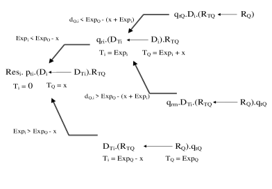
Figure 10: Backward search for multiple simultaneous events

Figure 10, shows the backward branching search, with the timer values at each step and the condition for each branch. In the first state, the timer $T_{Q}$ starts at an arbitrary point in time $x$, and the timer $T_{i}$ is set to ‘0’ (i.e. the timer expired triggering a response $p_{t_{i}}$). One step backward, either the timer at $i$ must have been started ‘$Exp_{Q}-x$’ units in the past, or the response timer must have been started ‘$Exp_{i}$’ units in the past. Depending on the relative values of these times some branch(es) become valid. The timer values at each step are updated accordingly. Note that if a timer expires while a message is in flight (i.e. transmitted but not yet received), we use the $m$ subscript to denote it is still multicast, as in $q_{r_{m}}$ in the figure.

Sometimes, the values of the timers and the delays are given as ranges or intervals. Following we present how branching decision are made when comparing intervals.

Branching decision for intervals

In order to conduct the search for multiple stimuli, we need to check the constraints for each branch. To decide on the branches valid for search, we compare values of timers and delays. These values are often given as intervals, e.g. $[a,b]$.

Comparison of two intervals $Int_{1}=[a_{1},b_{1}]$ and $Int_{2}=[a_{2},b_{2}]$ is done according to the following rules.

Branch $Int_{1}>Int_{2}$ becomes valid if there exists a value in $[a_{1},b_{1}]$ that is greater than a value in $[a_{2},b_{2}]$, i.e. if there is overlap of more than one number between the intervals. We define the ‘$<$’ and ‘$=$’ relations similarly, i.e., if there are any numbers in the interval that satisfy the relation then the branch becomes valid.

For example, if we have the following branch conditions: (i) $Exp_{i}<Exp_{j}$, (ii) $Exp_{i}=Exp_{j}$, and (iii) $Exp_{i}>Exp_{j}$. If $Exp_{i}=[3,5]$ and $Exp_{j}=[4,6]$, then, according to our above definitions, all the branch conditions are valid. However, if $Exp_{i}=[3,5]$ and $Exp_{j}=[5,7]$, then only branches (i) and (ii) are valid.

The above definitions are sufficient to cover the forward search branching. However, for backward search branching, we may have an arbitrary value $x$ as noted above.

For example, take the state $(D_{i}\leftarrow D_{T_{i}}).R_{T_{Q}}$. Consider the timer at $Q$, the expiration duration of which is $Exp_{Q}$ and the value of which is $x$, and the timer at $i$, the expiration duration of which is $Exp_{i}$ and the value of which is ‘0’, as given in figure 10. Depending on the relevant values of $Exp_{i}$ and $Exp_{Q}-x$ the search follows some branch(es). If $Exp_{Q}=[a_{1},b_{1}]$, then $x=[0,b_{1}]$ and $Exp_{Q}-x=[0,b_{1}]$. Hence, we can apply the forward branching rules described earlier by taking $Exp_{Q}-x=[0,b_{1}]$, as follows. Since $Exp_{i}=[a_{2},b_{2}]$, where $a_{2}>0$ and $b_{2}>0$, hence, the branch condition $Exp_{i}>Exp_{Q}-x$ is always true. The condition $Exp_{i}=Exp_{Q}-x$ is valid when: (i) $Exp_{i}=Exp_{Q}$, or (ii) $Exp_{i}<Exp_{Q}$. The last condition, $Exp_{i}<Exp_{Q}-x$, is valid only if $Exp_{i}<Exp_{Q}$.

These rules are integrated into the search algorithm for our method to deal with multiple stimuli and timers simultaneously.

Appendix D Example Case Studies

In this section, we present several case studies that show how to apply the previous analysis results to examples in reliable multicast and related protocol design problems.

D.1 Topology Synthesis

In this subsection we apply the test synthesis method to the task where the timer values are known and the topology (i.e., $D$ matrix) is to be synthesized according to the worst-case behavior. We explore various timer settings. We investigate two examples of topology synthesis, one uses timers with fixed randomization intervals and the other uses timers that are a function of distance.

Let $Q$ be the requester and $1$, $2$ and $3$ be potential responders. Let $V_{t_{i}}$ be the time required for system $i$ to trigger a response transmission from the time a request was sent, i.e., $V_{t_{i}}=d_{Q,i}+Exp_{i}$. From Section 5, we get $V_{t_{i}}<V_{t_{j}}+d_{j,i}$ for worst-case overhead.

At time $t_{0}$ $Q$ sends the request. For simplicity we assume, without loss of generality, that the systems are ordered such that $V_{t_{i}}<V_{t_{j}}$ for $i<j$ (e.g., system $1$ has the least $d_{Q,1}+Exp_{1}$, then 2, and then 3). Thus the inequalities $V_{t_{i}}<V_{t_{j}}+d_{j,i}$ are readily satisfied for $i<j$ and we need only satisfy it for $i>j$.

From equation (1) for the worst-case (see Section 5) we get:

$$V_{t_{2}}<V_{t_{1}}+d_{1,2},$$

$$V_{t_{3}}<V_{t_{1}}+d_{1,3},$$

$$V_{t_{3}}<V_{t_{2}}+d_{2,3}.$$ (5)

By satisfying these inequalities we obtain the delay settings of the worst case topology, as will be shown in the rest of this section.

D.1.1 Timers with fixed randomization intervals

Some multicast applications and protocols (such as wb [4], IGMP [3] or PIM [42]) employ fixed randomization intervals to set the suppression timers. For instance, for the shared white board (wb) [4], the response timer is assigned a random value from the (uniformly distributed) interval [t,2*t] where t = 100 msec for the source $src$, and 200 msec for other responders.

Assume $Q$ is a receiver with a lost packet. Using wb parameters we get $Exp_{src}=[100,200]$ msec, and $Exp_{i}=[200,400]$ msec for all other nodes.

To derive worst-case topologies from inequalities (A.1) we may use a standard mathematical tool for linear or non-linear programming, for more details see Appendix B. However, in the following we illustrate general techniques that may be used to obtain the solution.

From inequalities (A.1) we get:

$d_{Q,2}+Exp_{2}=V_{t_{2}}<V_{t_{1}}+d_{1,2}=d_{Q,1}+Exp_{1}+d_{1,2}$.

This can be rewritten as

$$d_{Q,2}-(d_{Q,1}+d_{1,2})<Exp_{1}-Exp_{2}=diff_{1,2},$$ (6)

where

$$diff_{1,2}=\begin{cases}$[100,200] - [200,400] = [-300,0]$&\text{if 1 is src},\\ $[200,400] - [100,200] = [0,300]$&\text{if 2 is src},\\ $[200,400] - [200,400] = [-200,200]$&\text{Otherwise}.\end{cases}$$

Similarly, we derive the following from inequalities for $V_{t_{3}}$:

$d_{Q,3}-(d_{Q,1}+d_{1,3})<diff_{1,3}$, and

$d_{Q,3}-(d_{Q,2}+d_{2,3})<diff_{2,3}$.

If we assume system 1 to be the source, and for a conservative solution we choose the minimum value of $diff$, we get:

$min(diff_{1,2})=min(diff_{1,3})=-300$,

$min(diff_{2,3})=-200$.

We then substitute these values in the above inequalities, and assign the values of some of the delays to compute the others.

Example: if we assign $d_{Q,1}=d_{Q,2}=d_{Q,3}=100$msec, we get: $d_{1,2}>300$, $d_{1,3}>300$ and $d_{2,3}>200$.

These delays exhibit worst-case behavior for the timer suppression mechanism.

D.1.2 Timers as function of distance

In contrast to fixed timers, this section uses timers that are function of an estimated distance. The expiration timer may be set as a function of the distance to the requester. For example, system $i$ may set its timer to repond to a request from system $Q$ in the interval: $[C_{1}*E_{i,Q},(C_{1}+C_{2})*E_{i,Q}]$, where $E_{i,Q}$ is the estimated distance/delay from $i$ to $Q$, which is calculated using message exchange (e.g. SRM session messages) and is equal to $(d_{i,Q}+d_{Q,i})/2$. (Note that this estimate assumes symmetry which sometimes is not valid.)

[4] suggests values for $C_{1}$ and $C_{2}$ as 1 or $log_{10}G$, where $G$ is the number of members in the group.

We take $C_{1}=C_{2}=1$ to synthesize the worst-case topology. We get the expression

$Exp_{1}-Exp_{2}=[(d_{1,Q}+d_{Q,1})/2,d_{1,Q}+d_{Q,1}]-[(d_{2,Q}+d_{Q,2})/2,d_{2,Q}+d_{Q,2}]$.

Example: If we assume that $d_{1,Q}=d_{Q,1}=d_{2,Q}=d_{Q,2}=100msec$, we can rewrite the above relation as $Exp_{1}-Exp_{2}=[-100,100]$ msec.

Substituting in equation (A.2) above, we get $d_{1,2}>100$msec. Under similar assumptions, we can obtain $d_{2,3}>100$msec, and $d_{1,3}>100$msec.

Topologies with the above delay settings will experience the worst case overhead behavior (as defined above) for the timer suppression mechanism.

As was shown, the inequalities formulated automatically by our method in section 5, can be used with various timer strategies (e.g., fixed timers or timers as function of distance). Although the topologies we have presented are limited, a mathematical tool (such as LINDO) can be used to obtain solutions for larger topologies.

D.2 Timer configuration

In this subsection we give simple examples of the timer configuration task solution, where the delay bounds (i.e., D matrix) are given and the timer values are adjusted to achieve the required behavior.

In these examples the delay is given as an interval [x,y] msec. We show an example for worst-case analysis.

D.2.1 Worst-case analysis

If the given ranges for the delays are [2,200] msec for all delays, then the term $d_{Q,j}-d_{Q,i}+d_{j,i}$ evaluates to [-196,398]. From equation (A.2) above, we get

$Exp_{i}<Exp_{j}-196$, to guarantee that a response is triggered.

If the delays are [5,50] msec, we get:

$$Exp_{i}<Exp_{j}-45,$$

i.e., $i$’s expiration timer must be less than $j$’s by at least 45 msecs. Note that we have an implied inequality that $Exp_{i}>0$ for all $i$.

These timer expiration settings would exhibit worst-case behavior for the given delay bounds.

References

- [1] D. Estrin, D. Farinacci, A. Helmy, D. Thaler, S. Deering, M. Handley, V. Jacobson, C. Liu, P. Sharma, and L. Wei. Protocol Independent Multicast - Sparse Mode (PIM-SM): Protocol Specification. IETF RFC 2362., June 1998.
- [2] D. Estrin, D. Farinacci, A. Helmy, V. Jacobson, and L. Wei. Protocol Independent Multicast - Dense Mode (PIM-DM): Protocol Specification. IETF Proposed RFC, September 1996.
- [3] W. Fenner. Internet Group Management Protocol, Version 2. IDMR Internet-Draft proposed standard, November 1997.
- [4] S. Floyd, V. Jacobson, C. Liu, S. McCanne, and L. Zhang. A Reliable Multicast Framework for Light-weight Sessions and Application Level Framing. IEEE/ACM Transactions on Networking, November 1996.
- [5] K. Miller, K. Robertson, A. Tweedly, and M. White. StarBurst Multicast File Transfer Protocol (MFTP) Specification. Internet-Draft, 1998.
- [6] R. Govindan, H. Yu, and D. Estrin. Large-scale weakly consistent replication using multicast. USC-CS-TR-98-682, Sep 1998.
- [7] H. Yu, L. Breslau, and S. Shenker. A scalable web cache consistency architecture. ACM SIGCOMM, 1999.
- [8] L. Zhang, S. Michel, K. Nguyen, A. Rosenstein, S. Floyd, and V. Jacobson. Adaptive Web Caching: Towards a New Global Caching Architecture. 3rd International WWW Caching Workshop, June 1998.
- [9] M. Handley. Session Directories and Scalable Internet Multicast Address Allocation. ACM SIGCOMM, 1998.
- [10] Elan Amir, Steve McCanne, and Randy Katz. An active service framework and its application to real-time multimedia transcoding. ACM SIGCOMM’98, September 1998.
- [11] A. Reddy, R. Govindan, and D. Estrin. Fault Isolation in Multicast Trees. ACM SIGCOMM, 2000.
- [12] J. Atwood, O. Catrina, J. Fenton, and W. Strayer. Reliable Multicasting in the Xpress Transport Protocol. Proceedings of the 21st Local Computer Networks Conference, October 1996.
- [13] H. Schulzrinne, S. Casner, R. Frederick, and V. Jacobson. RTP: A Transport Protocol for Real-Time Applications. RFC 1889, January 1996.
- [14] A. Helmy and D. Estrin. Simulation-based STRESS Testing Case Study: A Multicast Routing Protocol. Sixth International Symposium on Modeling, Analysis and Simulation of Computer and Telecommunication Systems (MASCOTS ’98), July 1998.
- [15] Ahmed Helmy, Deborah Estrin, and Sandeep Gupta. Fault-oriented test generation for multicast routing protocol design. Formal Description Techniques (FORTE XI) & Protocol Specification, Testing, and Verification (PSTV XVIII), 1998 IFIP TC6/WG6.1 Joint International Conference, Paris, France., November 1998.
- [16] L. Breslau, D. Estrin, K. Fall, S. Floyd, J. Heidemann, A. Helmy, P. Huang, S. McCanne, K. Varadhan, H. Yu, and Y. Xu. Advances in Network Simulation. IEEE Computer, May 2000.
- [17] K. Calvert, M. Doar, and E. Zegura. Modeling Internet Topology. IEEE Communications, 1997.
- [18] K. Varadhan, D. Estrin, and S. Floyd. Impact of Network Dynamics on End-to-End Protocols: Case Studies in Reliable Multicast. ISCC98, 1998.
- [19] P. Huang, D. Estrin, and J. Heidemann. Enabling Large-Scale Simulations: Selective Abstraction Approach to The Study of Multicast Protocols. Sixth International Symposium on Modeling, Analysis and Simulation of Computer and Telecommunication Systems (MASCOTS ’98), July 1998.
- [20] A. Helmy, D. Estrin, and S. Gupta. Systematic Testing of Multicast Routing Protocol Robustness: Analysis of Forward and Backward Search Techniques. IEEE Int’l Conf. on Computer Communications and Networks (IC3N), October 2000.
- [21] S. Begum, M. Sharma, A. Helmy, and S. Gupta. Systematic Testing of Protocol Robustness: Case Studies on Mobile IP and MARS. IEEE Conf. on Local Computer Networks (LCN), November 2000.
- [22] K. Seada, S. Gupta, and A. Helmy. Systematic Evaluation of Multicast Congestion Control Protocols. SCS International Symposium on Performance Evaluation of Computer and Telecommunication Systems (SPECTS), July 2002.
- [23] K. Seada and A. Helmy. Fairness Evaluation Experiments for Multicast Congestion Control Protocols. IEEE GLOBECOM, November 2002.
- [24] K. Saleh, I. Ahmed, K. Al-Saqabi, and A. Agarwal. A recovery approach to the design of stabilizing communication protocols. Journal of Computer Communication, Vol. 18, No. 4, pages 276–287, April 1995.
- [25] E. Clarke and J. Wing. Formal Methods: State of the Art and Future Directions. ACM Workshop on Strategic Directions in Computing Research, Vol. 28, No. 4, pages 626–643, December 1996.
- [26] R. Boyer and J. Moore. A Computational Logic Handbook. Academic Press, Boston, 1988.
- [27] J. Spivey. Understanding Z: a Specification Language and its Formal Semantics. Cambridge University Press, 1988.
- [28] F. Lin, P. Chu, and M. Liu. Protocol Verification using Reachability Analysis. Computer Communication Review, Vol. 17, No. 5, 1987.
- [29] P. Godefroid. Using partial orders to improve automatic verification methods. Proc. 2nd Workshop on Computer-Aided Verification, Springer Verlag, New York, 1990.
- [30] F. Pong and M. Dubois. Verification Techniques for Cache Coherence Protocols. ACM Computing Surveys, Volume 29, No. 1, pages 82–126, March 1996.
- [31] Mihalis Yannakakis and David Lee. Testing Finite State Machines: Fault Detection. Journal of Computer and Systems Sciences, 1995.
- [32] D. Rayner. OSI conformance testing. Computer Networks and ISDN Systems, Special issue on Conformance Testing, Vol. 14, No. 1, pages 79–98, 1987.
- [33] K. Sabnani and A. Dahbura. A new technique for generating protocol tests. ACM Computer Communication Review, Vol. 15, No. 4, September 1985.
- [34] K. Sabnani and A. Dahbura. A protocol test generation procedure. Computer Networks and ISDN Systems, Vol. 15, 1988.
- [35] M. Abramovici, M. Breuer, and A. Friedman. Digital Systems Testing and Testable Design. AT & T Labs., 1990.
- [36] S. Bajaj, L. Breslau, D. Estrin, K. Fall, S. Floyd, P. Haldar, M. Handley, A. Helmy, J. Heidemann, P. Huang, S. Kumar, S. McCanne, R. Rejaie, P. Sharma, S. Shenker, K. Varadhan, H. Yu, Y. Xu, and D. Zappala. Virtual InterNetwork Testbed: Status and research agenda. USC-CS-TR 98-678, July 1998.
- [37] D. Estrin, M. Handley, J. Heidemann, S. McCanne, Y. Xu, and H. Yu. Network Visualization with the VINT Network Animator Nam. To Appear in IEEE Computer Magazine, November 1999.
- [38] D. Estrin, R. Govindan, J. Heidemann, and S. Kumar. Scalable coordination in sensor networks. MobiCOM, August 1999.
- [39] N. Karmarkar. A new polynomial-time algorithm for linear programming. Combinatorica, pages 373–395, 1984.
- [40] G. Dantzig. Simplex Method for Solving Linear Programs. The Macmillian Press, Ltd., London, 1987.
- [41] B. Borchers and J. Mitchell. An Improved Branch and Bound Algorithm for Mixed Integer Nonlinear Programs. Computers and Operations Research, 1994.
- [42] D. Estrin, D. Farinacci, A. Helmy, D. Thaler, S. Deering, M. Handley, V. Jacobson, C. Liu, P. Sharma, and L. Wei. Protocol Independent Multicast - Sparse Mode (PIM-SM): Motivation and Architecture. IETF Proposed RFC., October 1996.