Optimal Ordered Problem Solver

Abstract

In a quite pragmatic sense oops is the fastest general way of solving one task after another, always optimally exploiting solutions to earlier tasks when possible. It can be used for increasingly hard problems of optimization or prediction. Suppose there is only one task and a bias in form of a probability distribution $P$ on programs for a universal computer. In the $i$-th phase $(i=1,2,3,\ldots)$ of asymptotically optimal nonincremental universal search (Levin, 1973, 1984) we test all programs $p$ with runtime $\leq 2^{i}P(p)$ until the task is solved. Now suppose there is a sequence of tasks, e.g., the $n$-th task is to find a shorter path through a maze than the best found so far. To reduce the search time for new tasks, previous incremental extensions of universal search tried to modify $P$ through experience with earlier tasks—but in a heuristic and non-general and suboptimal way prone to overfitting. Oops, however, does it right.

Tested self-delimiting program prefixes (beginnings of code that may continue) are immediately executed while being generated. They grow by one instruction whenever they request this. The storage for the first found program computing a solution to the current task becomes non-writeable. Programs tested during search for solutions to later task may copy non-writeable code into separate modifiable storage, to edit it and execute the modified result. Prefixes may also recompute the probability distribution on their suffixes in arbitrary computable ways. To solve the $n$-th task we sacrifice half the total search time for testing (via universal search) programs that have the most recent successful program as a prefix. The other half remains for testing fresh programs starting at the address right above the top non-writeable address. When we are searching for a universal solver for all tasks in the sequence we have to time-share the second half (but not the first!) among all tasks $1..n$. For realistic limited computers we need efficient backtracking in program space to reset storage contents modified by tested programs. We introduce a recursive procedure for doing this in time-optimal fashion.

Oops can solve tasks unsolvable by traditional reinforcement learners and AI planners, such as Towers of Hanoi with 30 disks (minimal solution size $>10^{9}$). In our experiments OOPS demonstrates incremental learning by reusing previous solutions to discover a prefix that temporarily rewrites the distribution on its suffixes, such that universal search is accelerated by a factor of 1000. This illustrates how oops can benefit from self-improvement and metasearching, that is, searching for faster search procedures.

We mention several oops variants and outline oops-based reinforcement learners. Since oops will scale to larger problems in essentially unbeatable fashion, we also examine its physical limitations.

Keywords: oops, bias-optimality, incremental optimal universal search, efficient planning & backtracking in program space, metasearching & metalearning, self-improvement

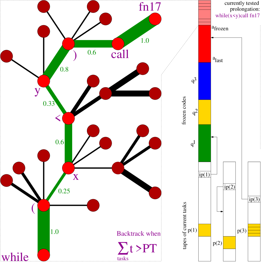
Figure 2: Search tree during an oops application; compare Section 4.1 and Figure 1. The tree branches are program prefixes (a single prefix may modify several task-specific tapes in parallel); nodes represent tokens; widths of connections between nodes stand for temporary, task-specific transition probabilities encoded on the modifiable tapes. Prefixes may contain (or call previously frozen) subprograms that dynamically modify the conditional probabilities during runtime, thus rewriting the suffix search procedure. In the example, the currently tested prefix (above the previously frozen codes) consists of the token sequence while $(x<y)$ call fn17 (real values denote transition probabilities). Here fn17 might be a time-consuming primitive, say, for manipulating the arm of a realistic virtual robot. Before requesting an additional token, this prefix may run for a long time, thus changing many components of numerous tapes. Node-oriented backtracking through procedure Try will restore partially solved task sets and modifications of internal states and continuation probabilities once          there is an error or the sum of the runtimes of the current prefix on all current tasks exceeds the prefix probability multiplied by the total search time so far. See text for details.

Based on arXiv:cs.AI/0207097 v1 (TR-IDSIA-12-02 version 1.0, July 2002) (Schmidhuber, 2002d, a). All sections are illustrated by Figures 1 and 2 at the end of this paper. Frequently used symbols are collected in reference Table 1 (general oops-related symbols) and Table 2 (less important implementation-specific symbols, explained in the appendix, Section A).

1 Introduction

We train children and most machine learning systems on sequences of harder and harder tasks. This makes sense since new problems often are more easily solved by reusing or adapting solutions to previous problems.

Often new tasks depend on solutions for earlier tasks. For example, given an NP-hard optimization problem, the $n$-th task in a sequence of tasks may be to find an approximation to the unknown optimal solution such that the new approximation is at least 1 % better (according to some measurable performance criterion) than the best found so far.

Alternatively we may want to find a strategy for solving all tasks in a given sequence of more and more complex tasks. For example, we might want to teach our learner a program that computes fac$(n)=1\times 2\times\ldots n$ for any given positive integer $n$. Naturally, the $n$-th task in the “training sequence” will be to compute fac$(n)$.

In general we would like our learner to continually profit from useful information conveyed by solutions to earlier tasks. To do this in an optimal fashion, the learner may also have to improve the way it exploits earlier solutions. Is there a general yet time-optimal way of achieving such a feat? Indeed, there is. The Optimal Ordered Problem Solver (oops) is a simple, general, theoretically sound way of solving one task after another, efficiently searching the space of programs that compute solution candidates, including programs that organize and manage and adapt and reuse earlier acquired knowledge.

1.1 Overview

Section 2 will survey previous relevant work on general optimal search algorithms. Section 3 will use the framework of universal computers to explain oops and how it benefits from incrementally extracting useful knowledge hidden in training sequences. The remainder of the paper is devoted to “Realistic” oops which uses a recursive procedure for time-optimal planning and backtracking in program space to perform efficient storage management (Section 4) on realistic, limited computers. Appendix A describes an pilot implementation of Realistic oops based on a stack-based universal programming language inspired by Forth (Moore and Leach, 1970), with initial primitives for defining and calling recursive functions, iterative loops, arithmetic operations, domain-specific behavior, and even for rewriting the search procedure itself. Experiments in Section 6 use the language of Appendix A to solve 60 tasks in a row: we first teach oops something about recursion, by training it to construct samples of the simple context free language $\{1^{k}2^{k}\}$ ($k$ 1’s followed by $k$ 2’s), for $k$ up to 30. This takes roughly 0.3 days on a standard personal computer (PC). Thereafter, within a few additional days, oops demonstrates the benefits of incremental knowledge transfer: it exploits certain properties of its previously discovered universal $1^{k}2^{k}$-solver to greatly accelerate the search for a universal solver for all $k$ disk Towers of Hanoi problems, solving all instances up to $k=30$ (solution size $2^{k}-1$). Previous, less general reinforcement learners and nonlearning AI planners tend to fail for much smaller instances.

2 Survey of Universal Search and Suboptimal Incremental Extensions

Let us start by briefly reviewing general, asymptotically optimal search methods by Levin (1973, 1984) and Hutter (2002a). These methods are nonincremental in the sense that they do not attempt to accelerate the search for solutions to new problems through experience with previous problems. We will point out drawbacks of existing heuristic extensions for incremental search. The remainder of the paper will describe oops which overcomes these drawbacks.

2.1 Bias-Optimality

For the purposes of this paper, a problem $r$ is defined by a recursive procedure $f_{r}$ that takes as an input any potential solution (a finite symbol string $y\in Y$, where $Y$ represents a search space of solution candidates) and outputs 1 if $y$ is a solution to $r$, and 0 otherwise. Typically the goal is to find as quickly as possible some $y$ that solves $r$.

Define a probability distribution $P$ on a finite or infinite set of programs for a given computer. $P$ represents the searcher’s initial bias (e.g., $P$ could be based on program length, or on a probabilistic syntax diagram). A bias-optimal searcher will not spend more time on any solution candidate than it deserves, namely, not more than the candidate’s probability times the total search time:

Definition 1 (Bias-Optimal Searchers)

Given is a problem class $\cal R$, a search space $\cal C$ of solution candidates (where any problem $r\in\cal R$ should have a solution in $\cal C$), a task-dependent bias in form of conditional probability distributions $P(q\mid r)$ on the candidates $q\in\cal C$, and a predefined procedure that creates and tests any given $q$ on any $r\in\cal R$ within time $t(q,r)$ (typically unknown in advance). A searcher is $n$-bias-optimal ($n\geq 1$) if for any maximal total search time $T_{max}>0$ it is guaranteed to solve any problem $r\in\cal R$ if it has a solution $p\in\cal C$ satisfying $t(p,r)\leq P(p\mid r)~{}T_{max}/n$. It is bias-optimal if $n=1$.

This definition makes intuitive sense: the most probable candidates should get the lion’s share of the total search time, in a way that precisely reflects the initial bias.

2.2 Near-Bias-Optimal Nonincremental Universal Search

The following straight-forward method (sometimes referred to as Levin Search or Lsearch) is near-bias-optimal. For simplicity, we notationally suppress conditional dependencies on the current problem. Compare Levin (1973, 1984), Solomonoff (1986), Schmidhuber et al. (1997b), Li and Vitányi (1997), Hutter (2002a) (Levin also attributes similar ideas to Allender):

Method 2.1 (Lsearch)

Set current time limit T=1. While problem not solved do:

Test all programs $q$ such that $t(q)$, the maximal time spent on creating and running and testing $q$, satisfies $t(q)<P(q)~{}T$. Set $T:=2T.$

Note that Lsearch has the optimal order of computational complexity: Given some problem class, if some unknown optimal program $p$ requires $f(k)$ steps to solve a problem instance of size $k$, then Lsearch will need at most $O(P(p)f(k))=O(f(k))$ steps — the constant factor $P(p)$ may be huge but does not depend on $k$.

The near-bias-optimality of Lsearch is hardly affected by the fact that for each value of $T$ we repeat certain computations for the previous value. Roughly half the total search time is still spent on $T$’s maximal value (ignoring hardware-specific overhead for parallelization and nonessential speed-ups due to halting programs if there are any). Note also that the time for testing is properly taken into account here: any result whose validity is hard to test is automatically penalized.

Universal Lsearch provides inspiration for nonuniversal but very practical methods which are optimal with respect to a limited search space, while suffering only from very small slowdown factors. For example, designers of planning procedures often just face a binary choice between two options such as depth-first and breadth-first search. The latter is often preferrable, but its greater demand for storage may eventually require to move data from on-chip memory to disk. This can slow down the search by a factor of 10,000 or more. A straightforward solution in the spirit of Lsearch is to start with a 50 % bias towards either technique, and use both depth-first and breadth-first search in parallel — this will cause a slowdown factor of at most 2 with respect to the best of the two options (ignoring a bit of overhead for parallelization). Such methods have presumably been used long before Levin’s 1973 paper. Wiering and Schmidhuber (1996) and Schmidhuber et al. (1997b) used rather general but nonuniversal variants of Lsearch to solve machine learning toy problems unsolvable by traditional methods. Probabilistic alternatives based on probabilistically chosen maximal program runtimes in Speed-Prior style (Schmidhuber, 2000, 2002e) also outperformed traditional methods on toy problems (Schmidhuber, 1995, 1997).

2.3 Asymptotically Fastest Nonincremental Problem Solver

Recently my postdoc Hutter (2002a) developed a more complex asymptotically optimal search algorithm for all well-defined problems. Hsearch (or Hutter Search) cleverly allocates part of the total search time to searching the space of proofs for provably correct candidate programs with provable upper runtime bounds; at any given time it focuses resources on those programs with the currently best proven time bounds. Unexpectedly, Hsearch manages to reduce the constant slowdown factor to a value smaller than $5$. In fact, it can be made smaller than $1+\epsilon$, where $\epsilon$ is an arbitrary positive constant (M. Hutter, personal communication, 2002).

Unfortunately, however, Hsearch is not yet the final word in computer science, since the search in proof space introduces an unknown additive problem class-specific constant slowdown, which again may be huge. While additive constants generally are preferrable to multiplicative ones, both types may make universal search methods practically infeasible—in the real world constants do matter. For example, the last to cross the finish line in the Olympic 100 m dash may be only a constant factor slower than the winner, but this will not comfort him. And since constants beyond $2^{500}$ do not even make sense within this universe, both Lsearch and Hsearch may be viewed as academic exercises demonstrating that the $O()$ notation can sometimes be practically irrelevant despite its wide use in theoretical computer science.

2.4 Previous Work on Incremental Extensions of Universal Search

“Only math nerds would consider $2^{500}$ finite.” (Leonid Levin)

Hsearch and Lsearch (Sections 2.2, 2.3) neglect one potential source of speed-up: they are nonincremental in the sense that they do not attempt to minimize their constant slowdowns by exploiting experience collected in previous searches for solutions to earlier tasks. They simply ignore the constants — from an asymptotic point of view, incremental search does not buy anything.

A heuristic attempt (Schmidhuber et al., 1997b) to greatly reduce the constants through experience was called Adaptive Lsearch or Als — compare related ideas by Solomonoff (1986, 1989). Essentially Als works as follows: whenever Lsearch finds a program $q$ that computes a solution for the current problem, $q$’s probability $P(q)$ is substantially increased using a “learning rate,” while probabilities of alternative programs decrease appropriately. Subsequent Lsearches for new problems then use the adjusted $P$, etc. Schmidhuber et al. (1997b) and Wiering and Schmidhuber (1996) used a nonuniversal variant of this approach to solve reinforcement learning (RL) tasks in partially observable environments unsolvable by traditional RL algorithms.

Each Lsearch invoked by Als is bias-optimal with respect to the most recent adjustment of $P$. On the other hand, the rather arbitrary $P$-modifications themselves are not necessarily optimal. They might lead to overfitting in the following sense: modifications of $P$ after the discovery of a solution to problem 1 could actually be harmful and slow down the search for a solution to problem 2, etc. This may provoke a loss of near-bias-optimality with respect to the initial bias during exposure to subsequent tasks. Furthermore, Als has a fixed prewired method for changing $P$ and cannot improve this method by experience. The main contribution of this paper is to overcome all such drawbacks in a principled way.

2.5 Other Work on Incremental Learning

Since the early attempts of Newell and Simon (1963) at building a “General Problem Solver” —see also Rosenbloom et al. (1993)—much work has been done to develop mostly heuristic machine learning algorithms that solve new problems based on experience with previous problems, by incrementally shifting the inductive bias in the sense of Utgoff (1986). Many pointers to learning by chunking, learning by macros, hierarchical learning, learning by analogy, etc. can be found in the book by Mitchell (1997). Relatively recent general attempts include program evolvers such as Adate (Olsson, 1995) and simpler heuristics such as Genetic Programming (GP) (Cramer, 1985, Banzhaf et al., 1998). Unlike logic-based program synthesizers (Green, 1969, Waldinger and Lee, 1969, Deville and Lau, 1994), program evolvers use biology-inspired concepts of Evolutionary Computation (Rechenberg, 1971, Schwefel, 1974) or Genetic Algorithms (Holland, 1975) to evolve better and better computer programs. Most existing GP implementations, however, do not even allow for programs with loops and recursion, thus ignoring a main motivation for search in program space. They either have very limited search spaces (where solution candidate runtime is not even an issue), or are far from bias-optimal, or both. Similarly, traditional reinforcement learners (Kaelbling et al., 1996) are neither general nor close to being bias-optimal.

A first step to make GP-like methods bias-optimal would be to allocate runtime to tested programs in proportion to the probabilities of the mutations or “crossover operations” that generated them. Even then there would still be room for improvement, however, since GP has quite limited ways of making new programs from previous ones—it does not learn better program-making strategies.

This brings us to several previous publications on learning to learn or metalearning (Schmidhuber, 1987), where the goal is to learn better learning algorithms through self-improvement without human intervention—compare the human-assisted self-improver by Lenat (1983). We introduced the concept of incremental search for improved, probabilistically generated code that modifies the probability distribution on the possible code continuations: incremental self-improvers (Schmidhuber et al., 1997a) use the success-story algorithm SSA to undo those self-generated probability modifications that in the long run do not contribute to increasing the learner’s cumulative reward per time interval. An earlier meta-GP algorithm (Schmidhuber, 1987) was designed to learn better GP-like strategies; Schmidhuber (1987) also combined principles of reinforcement learning economies (Holland, 1985) with a “self-referential” metalearning approach. A gradient-based metalearning technique (Schmidhuber, 1993) for continuous program spaces of differentiable recurrent neural networks (RNNs) was also designed to favor better learning algorithms; compare the remarkable recent success of the related but technically improved RNN-based metalearner by Hochreiter et al. (2001).

The algorithms above generally are not near-bias-optimal though. The method discussed in this paper, however, combines optimal search and incremental self-improvement, and will be $n$-bias-optimal, where $n$ is a small and practically acceptable number, such as 8.

3 OOPS on Universal Computers

An informed reader familiar with concepts such as universal computers (Turing, 1936) and self-delimiting programs (Levin, 1974, Chaitin, 1975) will probably understand the simple basic principles of oops by just reading the abstract. For the others, Subsection 3.1 will start the formal description of oops by introducing notation and explaining program sets that are prefix codes. Subsection 3.2 will provide oops pseudocode and point out its essential properties and a few essential differences to previous work. The remainder of the paper is about practical implementations of the basic principles on realistic computers with limited storage.

Symbol	Description
$Q$	variable set of instructions or tokens
$Q_{i}$	$i$-th possible token (an integer)
$n_{Q}$	current number of tokens
$Q^{*}$	set of strings over alphabet $Q$, containing the search space of programs
$q$	total current code $\in Q^{*}$
$q_{n}$	$n$-th token of code $q$
$q^{n}$	$n$-th frozen program $\in Q^{*}$, where total code $q$ starts with $q^{1}q^{2}\ldots$
$qp$	$q$-pointer to the highest address of code $q=q_{1:qp}$
$a_{last}$	start address of a program (prefix) solving all tasks so far
$a_{frozen}$	top frozen address, can only grow, $1\leq a_{last}\leq a_{frozen}\leq qp$
$q_{1:a_{frozen}}$	current code bias
$R$	variable set of tasks, ordered in cyclic fashion; each task has a computation tape
$S$	set of possible tape symbols (here: integers)
$S^{*}$	set of strings over alphabet $S$, defining possible states stored on tapes
$s^{i}$	an element of $S^{*}$
$s(r)$	variable state of task $r\in R$, stored on tape $r$
$s_{i}(r)$	$i$-th component of $s(r)$
$l(s)$	length of any string $s$
$z(i)(r)$	equal to $q_{i}$ if $0<i\leq l(q)$ or equal to $s_{-i}(r)$ if $-l(s(r))\leq i\leq 0$
$ip(r)$	current instruction pointer of task $r$, encoded on tape $r$ within state $s(r)$
$p(r)$	variable probability distribution on $Q$, encoded on tape $r$ as part of $s(r)$
$p_{i}(r)$	current history-dependent probability of selecting $Q_{i}$ if $ip(r)=qp+1$

Table 1: Symbols used to explain the basic principles of oops (Section 3).

3.1 Formal Setup and Notation

Unless stated otherwise or obvious, to simplify notation, throughout the paper newly introduced variables are assumed to be integer-valued and to cover the range implicit in the context. Given some finite or countably infinite alphabet $Q=\{Q_{1},Q_{2},\ldots\}$, let $Q^{*}$ denote the set of finite sequences or strings over $Q$, where $\lambda$ is the empty string. Then let $q,q^{1},q^{2},\ldots\in Q^{*}$ be (possibly variable) strings. $l(q)$ denotes the number of symbols in string $q$, where $l(\lambda)=0$; $q_{n}$ is the $n$-th symbol of string $q$; $q_{m:n}=\lambda$ if $m>n$ and $q_{m}q_{m+1}\ldots q_{n}$ otherwise (where $q_{0}:=q_{0:0}:=\lambda$). $q^{1}q^{2}$ is the concatenation of $q^{1}$ and $q^{2}$ (e.g., if $q^{1}=abc$ and $q^{2}=dac$ then $q^{1}q^{2}=abcdac$).

Consider countable alphabets $S$ and $Q$. Strings $s,s^{1},s^{2},\ldots\in S^{*}$ represent possible internal states of a computer; strings $q,q^{1},q^{2},\ldots\in Q^{*}$ represent token sequences or code or programs for manipulating states. We focus on $S$ being the set of integers and $Q:=\{1,2,\ldots,n_{Q}\}$ representing a set of $n_{Q}$ instructions of some universal programming language (Gödel, 1931, Turing, 1936). (The first universal programming language due to Gödel (1931) was based on integers as well, but ours will be more practical.) $Q$ and $n_{Q}$ may be variable: new tokens may be defined by combining previous tokens, just as traditional programming languages allow for the declaration of new tokens representing new procedures. Since $Q^{*}\subset S^{*}$, substrings within states may also encode programs.

$R$ is a set of currently unsolved tasks. Let the variable $s(r)\in S^{*}$ denote the current state of task $r\in R$, with $i$-th component $s_{i}(r)$ on a computation tape $r$ (a separate tape holding a separate state for each task, initialized with task-specific inputs represented by the initial state). Since subsequences on tapes may also represent executable code, for convenience we combine current code $q$ and any given current state $s(r)$ in a single address space, introducing negative and positive addresses ranging from $-l(s(r))$ to $l(q)+1$, defining the content of address $i$ as $z(i)(r):=q_{i}$ if $0<i\leq l(q)$ and $z(i)(r):=s_{-i}(r)$ if $-l(s(r))\leq i\leq 0$. All dynamic task-specific data will be represented at nonpositive addresses (one code, many tasks). In particular, the current instruction pointer ip(r) $:=z(a_{ip}(r))(r)$ of task $r$ (where $ip(r)\in{-l(s(r)),\ldots,l(q)+1})$ can be found at (possibly variable) address $a_{ip}(r)\leq 0$. Furthermore, $s(r)$ also encodes a modifiable probability distribution $p(r)=\{p_{1}(r),p_{2}(r),\ldots,p_{n_{Q}}(r)\}$ $(\sum_{i}p_{i}(r)=1)$ on $Q$.

Code is executed in a way inspired by self-delimiting binary programs (Levin, 1974, Chaitin, 1975) studied in the theory of Kolmogorov complexity and algorithmic probability (Solomonoff, 1964, Kolmogorov, 1965). Section 4.1 will present details of a practically useful variant of this approach. Code execution is time-shared sequentially among all current tasks. Whenever any $ip(r)$ has been initialized or changed such that its new value points to a valid address $\geq-l(s(r))$ but $\leq l(q)$, and this address contains some executable token $Q_{i}$, then $Q_{i}$ will define task $r$’s next instruction to be executed. The execution may change $s(r)$ including $ip(r)$. Whenever the time-sharing process works on task $r$ and $ip(r)$ points to the smallest positive currently unused address $l(q)+1$, $q$ will grow by one token (so $l(q)$ will increase by 1), and the current value of $p_{i}(r)$ will define the current probability of selecting $Q_{i}$ as the next token, to be stored at new address $l(q)$ and to be executed immediately. That is, executed program beginnings or prefixes define the probabilities of their possible suffixes. (Programs will be interrupted through errors or halt instructions or when all current tasks are solved or when certain search time limits are reached—see Section 3.2.)

To summarize and exemplify: programs are grown incrementally, token by token; their prefixes are immediately executed while being created; this may modify some task-specific internal state or memory, and may transfer control back to previously selected tokens (e.g., loops). To add a new token to some program prefix, we first have to wait until the execution of the prefix so far explicitly requests such a prolongation, by setting an appropriate signal in the internal state. Prefixes that cease to request any further tokens are called self-delimiting programs or simply programs (programs are their own prefixes). So our procedure yields task-specific prefix codes on program space: with any given task, programs that halt because they have found a solution or encountered some error cannot request any more tokens. Given a single task and the current task-specific inputs, no program can be the prefix of another one. On a different task, however, the same program may continue to request additional tokens.

$a_{frozen}\geq 0$ is a variable address that can increase but not decrease. Once chosen, the code bias $q_{0:a_{frozen}}$ will remain unchangeable forever — it is a (possibly empty) sequence of programs $q^{1}q^{2}\ldots$, some of them prewired by the user, others frozen after previous successful searches for solutions to previous task sets (possibly completely unrelated to the current task set $R$).

To allow for programs that exploit previous solutions, the instruction set $Q$ should contain instructions for invoking or calling code found below $a_{frozen}$, for copying such code into some $s(r)$, and for editing the copies and executing the results. Examples of such instructions will be given in the appendix (Section A).

3.2 Basic Principles of OOPS

Given a sequence of tasks, we solve one task after another in the given order. The solver of the $n$-th task $(n\geq 1)$ will be a program $q^{i}$ $(i\leq n)$ stored such that it occupies successive addresses somewhere between 1 and $l(q)$. The solver of the $1$st task will start at address 1. The solver of the $n$-th task $(n>1)$ will either start at the same address as the solver of the $n-1$-th task, or right after its end address. To find a universal solver for all tasks in a given task sequence, do:

Method 3.1 (oops)

FOR task index $n=1,2,\ldots$ DO:

1. Initialize current time limit $T:=2$.

2. Spend at most $T/2$ on a variant of Lsearch that searches for a program solving task $n$ and starting at the start address $a_{last}$ of the most recent successful code (1 if there is none). That is, the problem-solving program either must be equal to $q_{a_{last}:a_{frozen}}$ or must have $q_{a_{last}:a_{frozen}}$ as a prefix. If solution found, go to 5.

3. Spend at most $T/2$ on Lsearch for a fresh program that starts at the first writeable address and solves all tasks $1..n$. If solution found, go to 5.

4. Set $T:=2T$, and go to 2.

5. Let the top non-writeable address $a_{frozen}$ point to the end of the just discovered problem-solving program.

3.3 Essential Properties of OOPS

The following observations highlight important aspects of oops and point out in which sense oops is optimal.

Observation 3.1

A program starting at $a_{last}$ and solving task $n$ will also solve all tasks up to $n$.

Proof (exploits the nature of self-delimiting programs): Obvious for $n=1$. For $n>1$: By induction, the code between $a_{last}$ and $a_{frozen}$, which cannot be altered any more, already solves all tasks up to $n-1$. During its application to task $n$ it cannot request any additional tokens that could harm its performance on these previous tasks. So those of its prolongations that solve task $n$ will also solve tasks $1,\ldots,n-1$.

Observation 3.2

$a_{last}$ does not increase if task $n$ can be more quickly solved by testing prolongations of $q_{a_{last}:a_{frozen}}$ on task $n$, than by testing fresh programs starting above $a_{frozen}$ on all tasks up to $n$.

Observation 3.3

Once we have found an optimal solver for all tasks in the sequence, at most half of the total future time will be wasted on searching for faster alternatives.

Observation 3.4

Unlike the learning rate-based bias shifts of Als (Section 2.4), those of oops do not reduce the probabilities of programs that were meaningful and executable before the addition of any new $q^{i}$.

But consider formerly meaningless program prefixes trying to access code for earlier solutions when there weren’t any: such prefixes may suddenly become prolongable and successful, once some solutions to earlier tasks have been stored. That is, unlike with Als the acceleration potential of oops is not bought at the risk of an unknown slowdown due to nonoptimal changes of the underlying probability distribution through a heuristically chosen learning rate. As new tasks come along, oops remains near-bias-optimal with respect to the initial bias, while still being able to profit in from subsequent code bias shifts in an optimal way.

Observation 3.5

Given the initial bias and subsequent code bias shifts due to $q^{1},q^{2},\ldots,$ no bias-optimal searcher with the same initial bias will solve the current task set substantially faster than oops.

Ignoring hardware-specific overhead (e.g., for measuring time and switching between tasks), oops will lose at most a factor 2 through allocating half the search time to prolongations of $q_{a_{last}:a_{frozen}}$, and another factor 2 through the incremental doubling of time limits in Lsearch (necessary because we do not know in advance the final time limit).

Observation 3.6

If the current task (say, task $n$) can already be solved by some previously frozen program $q^{k}$, then the probability of a solver for task $n$ is at least equal to the probability of the most probable program computing the start address $a(q^{k})$ of $q^{k}$ and setting instruction pointer $ip(n):=a(q^{k})$.

Observation 3.7

As we solve more and more tasks, thus collecting and freezing more and more $q^{i}$, it will generally become harder and harder to identify and address and copy-edit useful code segments within the earlier solutions.

As a consequence we expect that much of the knowledge embodied by certain $q^{j}$ actually will be about how to access and copy-edit and otherwise use programs $q^{i}$ ($i<j$) previously stored below $q^{j}$.

Observation 3.8

Tested program prefixes may rewrite the probability distribution on their suffixes in computable ways (based on previously frozen $q^{i}$), thus temporarily redefining the search space structure of Lsearch, essentially rewriting the search procedure. If this type of metasearching for faster search algorithms is useful to accelerate the search for a solution to the current problem, then oops will automatically exploit this.

Since there is no fundamental difference between domain-specific problem-solving programs and programs that manipulate probability distributions and rewrite the search procedure itself, we collapse both learning and metalearning in the same time-optimal framework.

Observation 3.9

If the overall goal is just to solve one task after another, as opposed to finding a universal solver for all tasks, it suffices to test only on task $n$ in step 3.

For example, in an optimization context the $n$-th task usually is not to find a solver for all tasks in the sequence, but just to find an approximation to some unknown optimal solution such that the new approximation is better than the best found so far.

3.4 Summary

Lsearch is about optimal time-sharing, given one problem. Oops is about optimal time-sharing, given a sequence of problems. The basic principles of Lsearch can be explained in one line: time-share all program tests such that each program gets a constant fraction of the total search time. Those of oops require just a few more lines: use self-delimiting programs and freeze those that were successful; given a new task, spend a fixed fraction of the total search time on programs starting with the most recently frozen prefix (test only on the new task, never on previous tasks); spend the rest of the time on fresh programs (when looking for a universal solver, test them on all previous tasks).

Oops spends part of the total search time for a new problem on programs that exploit previous solutions in computable ways. If the new problem can be solved faster by copy-editing/invoking previous code than by solving the new problem from scratch, then oops will find this out. If not, then at least it will not suffer from the previous solutions.

If oops is so simple indeed, then why does the paper not end here but has 31 additional pages? The answer is: to describe the additional efforts required to make OOPS work on realistic limited computers, as opposed to universal machines.

4 OOPS on Realistic Computers

Unlike the Turing machines originally used to describe Lsearch and Hsearch, realistic computers have limited storage. So we need to efficiently reset storage modifications computed by the numerous programs oops is testing. Furthermore, our programs typically will be composed from more complex primitive instructions than those of typical Turing machines. In what follows we will address such issues in detail.

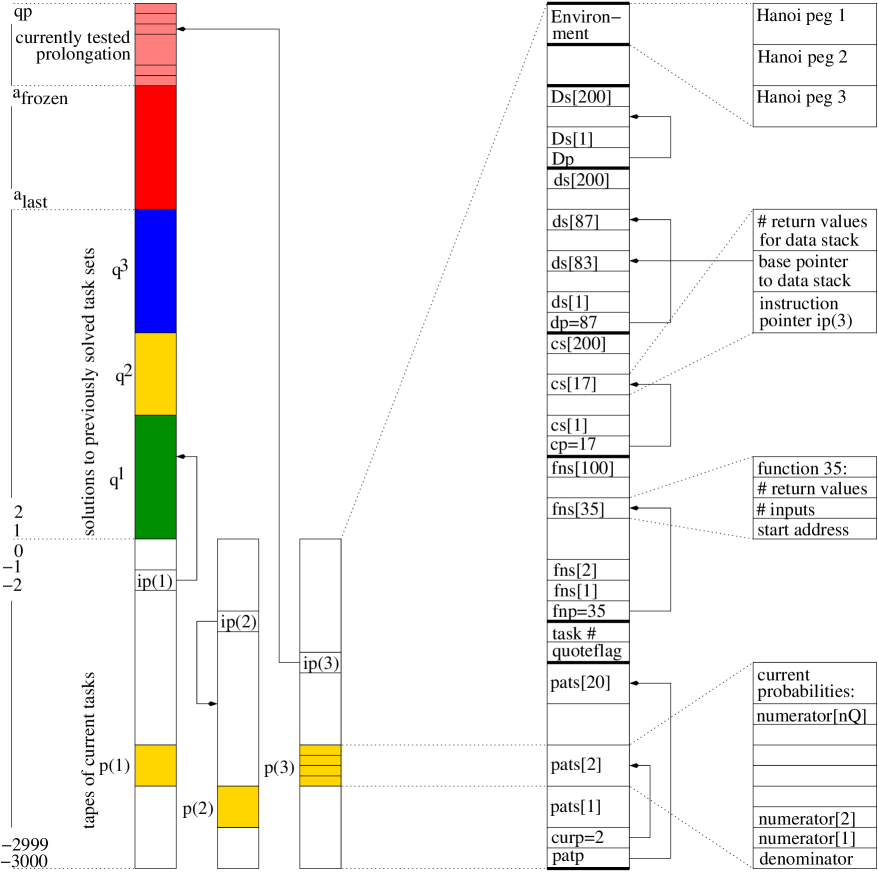
Figure 1: Storage snapshot during an oops application. Left: general picture (Section 3). Right: language-specific details for a particular Forth-like programming language (Sections A and 6). Left: current code $q$ ranges from addresses $1$ to $qp$ and includes previously frozen programs $q^{1},q^{2},q^{3}$. Three unsolved tasks require three tapes (lower left) with addresses $-3000$ to $0$. Instruction pointers $ip(1)$ and $ip(3)$ point to code in $q$, $ip(2)$ to code on the 2nd tape. Once, say, $ip(3)$ points right above the topmost address $qp$, the probability of the next instruction (at $qp+1$) is determined by the current probability distribution $p(3)$ on the possible tokens. oops spends equal time on programs starting with prefix $q_{a_{last}:a_{frozen}}$ (tested only on the most recent task, since such programs solve all previous tasks, by induction), and on all programs starting at $a_{frozen}+1$ (tested on all tasks). Right: Details of a single tape. There is space for several alternative self-made probability distributions on $Q$, each represented by $n_{Q}$ numerators and a common denominator. The pointer curp                   determines which distribution to use for the next token request. There is a stack fns of self-made function definitions, each with a pointer to its code’s start address, and its numbers of input arguments and return values expected on data stack ds (with stack pointer dp). The dynamic runtime stack cs handles all function calls. Its top entry holds the current instruction pointer ip and the current base pointer into ds below the arguments of the most recent call. There is also space for an auxiliary stack Ds, and for representing modifiable aspects of the environment.

4.1 Multitasking & Prefix Tracking By Recursive Procedure “Try”

Hsearch and Lsearch assume potentially infinite storage. Hence they may largely ignore questions of storage management. In any practical system, however, we have to efficiently reuse limited storage. Therefore, in both subsearches of Method 3.1 (steps 2 and 3), Realistic oops evaluates alternative prefix continuations by a practical, token-oriented backtracking procedure that can deal with several tasks in parallel, given some code bias in the form of previously found code.

The novel recursive method Try below essentially conducts a depth-first search in program space, where the branches of the search tree are program prefixes (each modifying a bunch of task-specific states), and backtracking (partial resets of partially solved task sets and modifications of internal states and continuation probabilities) is triggered once the sum of the runtimes of the current prefix on all current tasks exceeds the current time limit multiplied by the prefix probability (the product of the history-dependent probabilities of the previously selected prefix components in $Q$). This ensures near-bias-optimality (Def. 1), given some initial probabilistic bias on program space $\subseteq Q^{*}$.

Given task set $R$, the current goal is to solve all tasks $r\in R$, by a single program that either appropriately uses or extends the current code $q_{0:a_{frozen}}$ (no additional freezing will take place before all tasks in $R$ are solved).

4.1.1 Overview of “Try”

We assume an initial set of user-defined primitive behaviors reflecting prior knowledge and assumptions of the user. Primitives may be assembler-like instructions or time-consuming software, such as, say, theorem provers, or matrix operators for neural network-like parallel architectures, or trajectory generators for robot simulations, or state update procedures for multiagent systems, etc. Each primitive is represented by a token $\in Q$. It is essential that those primitives whose runtimes are not known in advance can be interrupted by oops at any time.

The searcher’s initial bias is also affected by initial, user-defined, task-dependent probability distributions on the finite or infinite search space of possible self-delimiting program prefixes. In the simplest case we start with a maximum entropy distribution on the tokens, and define prefix probabilities as the products of the probabilities of their tokens. But prefix continuation probabilities may also depend on previous tokens in context sensitive fashion defined by a probabilistic syntax diagram. In fact, we even permit that any executed prefix assigns a task-dependent, self-computed probability distribution to its own possible suffixes (compare Section 3.1).

Consider the left-hand side of Figure 1. All instruction pointers $ip(r)$ of all current tasks $r$ are initialized by some address, typically below the topmost code address, thus accessing the code bias common to all tasks, and/or using task-specific code fragments written into tapes. All tasks keep executing their instructions in parallel until interrupted or all tasks are solved, or until some task’s instruction pointer points to the yet unused address right after the topmost code address. The latter case is interpreted as a request for code prolongation through a new token, where each token has a probability according to the present task’s current state-encoded distribution on the possible next tokens. The deterministic method Try systematically examines all possible code extensions in a depth-first fashion (probabilities of prefixes are just used to order them for runtime allocation). Interrupts and backtracking to previously selected tokens (with yet untested alternatives) and the corresponding partial resets of states and task sets take place whenever one of the tasks encounters an error, or the product of the task-dependent probabilities of the currently selected tokens multiplied by the sum of the runtimes on all tasks exceeds a given total search time limit $T$.

To allow for efficient backtracking, Try tracks effects of tested program prefixes, such as task-specific state modifications (including probability distribution changes) and partially solved task sets, to reset conditions for subsequent tests of alternative, yet untested prefix continuations in an optimally efficient fashion (at most as expensive as the prefix tests themselves).

Since programs are created online while they are being executed, Try will never create impossible programs that halt before all their tokens are read. No program that halts on a given task can be the prefix of another program halting on the same task. It is important to see, however, that in our setup a given prefix that has solved one task (to be removed from the current task set) may continue to demand tokens as it tries to solve other tasks.

4.1.2 Details of “Try:” Bias-Optimal Depth-First Planning in Program Space

To allow us to efficiently undo state changes, we use global Boolean variables $mark_{i}(r)$ (initially False) for all possible state components $s_{i}(r)$. We initialize time $t_{0}:=0;$ probability $P:=1$; q-pointer $qp:=a_{frozen}$ and state $s(r)$ — including $ip(r)$ and $p(r)$ — with task-specific information for all task names $r$ in a so-called ring $R_{0}$ of tasks, where the expression “ring” indicates that the tasks are ordered in cyclic fashion; $\mid R\mid$ denotes the number of tasks in ring $R$. Given a global search time limit $T$, we Try to solve all tasks in $R_{0}$, by using existing code in $q=q_{1:qp}$ and / or by discovering an appropriate prolongation of $q$:

—————————————————————————————–

Method 4.1 (Boolean Try ($qp,r_{0},R_{0},t_{0},P$))

($r_{0}\in R_{0}$; returns True or False; may have the side effect of increasing $a_{frozen}$ and thus prolonging the frozen code $q_{1:a_{frozen}}$):

1. Make an empty stack $\cal S$; set local variables $r:=r_{0};R:=R_{0};t:=t_{0};$ Done$:=$ False.

While there are unsolved tasks ($\mid R\mid>0$) and there is enough time left ($t\leq PT$) and instruction pointer valid ($-l(s(r))\leq ip(r)\leq qp$) and instruction valid ($1\leq z(ip(r))(r)\leq n_{Q}$) and no halt condition is encountered (e.g., error such as division by 0, or robot bumps into obstacle; evaluate conditions in the above order until first satisfied, if any) Do:

Interpret / execute token $z(ip(r))(r)$ according to the rules of the given programming language, continually increasing $t$ by the consumed time. This may modify $s(r)$ including instruction pointer $ip(r)$ and distribution $p(r)$, but not code $q$. Whenever the execution changes some state component $s_{i}(r)$ whose $mark_{i}(r)=$ False, set $mark_{i}(r):=$ True and save the previous value $\hat{s}_{i}(r)$ by pushing the triple $(i,r,\hat{s}_{i}(r))$ onto $\cal S$. Remove $r$ from $R$ if solved. If $\mid R\mid>0$, set $r$ equal to the next task in ring $R$ (like in the round-robin method of standard operating systems). Else set Done $:=$ True; $a_{frozen}:=qp$ (all tasks solved; new code frozen, if any).

2. Use $\cal S$ to efficiently reset only the modified $mark_{i}(k)$ to False (the global mark variables will be needed again in step 3), but do not pop $\cal S$ yet.

3. If $ip(r)=qp+1$ (i.e., if there is an online request for prolongation of the current prefix through a new token): While Done $=$ False and there is some yet untested token $Z\in Q$ (untried since $t_{0}$ as value for $q_{qp+1}$) Do:

Set $q_{qp+1}:=Z$ and Done $:=$ Try ($qp+1,r,R,t,P*p(r)(Z)$), where $p(r)(Z)$ is $Z$’s probability according to current distribution $p(r)$.

4. Use $\cal S$ to efficiently restore only those $s_{i}(k)$ changed since $t_{0}$, thus restoring all tapes to their states at the beginning of the current invocation of Try. This will also restore instruction pointer $ip(r_{0})$ and original search distribution $p(r_{0})$. Return the value of Done.

—————————————————————————————–

A successful Try will solve all tasks, possibly increasing $a_{frozen}$ and prolonging total code $q$. In any case Try will completely restore all states of all tasks. It never wastes time on recomputing previously computed results of prefixes, or on restoring unmodified state components and marks, or on already solved tasks — tracking / undoing effects of prefixes essentially does not cost more than their execution. So the $n$ in Def. 1 of $n$-bias-optimality is not greatly affected by the undoing procedure: we lose at most a factor 2, ignoring hardware-specific overhead such as the costs of single push and pop operations on a given computer, or the costs of measuring time, etc.

Since the distributions $p(r)$ are modifiable, we speak of self-generated continuation probabilities. As the variable suffix $q^{\prime}:=q_{a_{frozen}+1:qp}$ of the total code $q=q_{1:qp}$ is growing, its probability can be readily updated:

$$P(q^{\prime}\mid s^{0})=\prod_{i=a_{frozen}+1}^{qp}P^{i}(q_{i}\mid s^{i}),$$ (1)

where $s^{0}$ is an initial state, and $P^{i}(q_{i}\mid s^{i})$ is the probability of $q_{i}$, given the state $s^{i}$ of the task $r$ whose variable distribution $p(r)$ (as a part of $s^{i}$) was used to determine the probability of token $q_{i}$ at the moment it was selected. So we allow the probability of $q_{qp+1}$ to depend on $q_{0:qp}$ and intial state $s^{0}$ in a fairly arbitrary computable fashion. Note that unlike the traditional Turing machine-based setup by Levin (1974) and Chaitin (1975) (always yielding binary programs $q$ with probability $2^{-l(q)}$) this framework of self-generated continuation probabilities allows for token selection probabilities close to 1.0, that is, even long programs may have high probability.

Example. In many programming languages the probability of token “(”, given a previous token “While”, equals 1. Having observed the “(” there is not a lot of new code to execute yet — in such cases the rules of the programming language will typically demand another increment of instruction pointer ip(r), which will lead to the request of another token through subsequent increment of the topmost code address. However, once we have observed a complete expression of the form “While (condition) Do (action),” it may take a long time until the conditional loop — interpreted via $ip(r)$ — is exited and the top address is incremented again, thus asking for a new token.

The round robin Try variant above keeps circling through all unsolved tasks, executing one instruction at a time. Alternative Try variants could also sequentially work on each task until it is solved, then try to prolong the resulting $q$ on the next task, and so on, appropriately restoring previous tasks once it turns out that the current task cannot be solved through prolongation of the prefix solving the earlier tasks. One potential advantage of round robin Try is that it will quickly discover whether the currently studied prefix causes an error for at least one task, in which case it can be discarded immediately.

Nonrecursive C-Code. An efficient iterative (nonrecursive) version of Try for a broad variety of initial programming languages was implemented in C. Instead of local stacks $\cal S$, a single global stack is used to save and restore old contents of modified cells of all tapes / tasks.

4.2 Realistic OOPS for Finding Universal Solvers

Recall that the instruction set $Q$ should contain instructions for invoking or calling code found below $a_{frozen}$, for copying such code into $s(r)$, and for editing the copies and executing the results (examples in Appendix A).

Now suppose there is an ordered sequence of tasks $r_{1},r_{2},\ldots$. Inductively suppose we have solved the first $n$ tasks through programs stored below address $a_{frozen}$, and that the most recently discovered program starting at address $a_{last}\leq a_{frozen}$ actually solves all of them, possibly using information conveyed by earlier programs $q^{1},q^{2},\ldots$. To find a program solving the first $n+1$ tasks, Realistic oops invokes Try as follows (using set notation for task rings, where the tasks are ordered in cyclic fashion—compare basic Method 3.1):

—————————————————————————————–

Method 4.2 (Realistic oops (n+1))

Initialize current time limit $T:=2$ and $q$-pointer $qp:=a_{frozen}$ (top frozen address).

1. Set instruction pointer $ip(r_{n+1}):=a_{last}$ (start address of code solving all tasks up to $n$).

If Try ($qp,r_{n+1},\{r_{n+1}\},0,\frac{1}{2}$) then exit.

(This means that half the search time is assigned to the most recent $q_{a_{last}:a_{frozen}}$ and all possible prolongations thereof).

2. If it is possible to initialize all $n+1$ tasks within time $T$:

Set local variable $a:=a_{frozen}+1$ (first unused address); for all $r\in\{r_{1},r_{2},\ldots,r_{n+1}\}$ set $ip(r):=a$. If Try ($qp,r_{n+1},\{r_{1},r_{2},\ldots,r_{n+1}\},0,\frac{1}{2}$) set $a_{last}:=a$ and exit.

(This means that half the time is assigned to all new programs with fresh starts).

3. Set $T:=2T$, and go to 1.

—————————————————————————————–

Therefore, given tasks $r_{1},r_{2},\ldots,$ first initialize $a_{last}$; then for $i:=1,2,\ldots$ invoke Realistic oops$(i)$ to find programs starting at (possibly increasing) address $a_{last}$, each solving all tasks so far, possibly eventually discovering a universal solver for all tasks in the sequence.

As address $a_{last}$ increases for the $n$-th time, $q^{n}$ is defined as the program starting at $a_{last}$’s old value and ending right before its new value. Program $q^{m}$ ($m>i,j$) may exploit $q^{i}$ by calling it as a subprogram, or by copying $q^{i}$ into some state $s(r)$, then editing it there, e.g., by inserting parts of another $q^{j}$ somewhere, then executing the edited variant.

4.3 Near-Bias-Optimality of Realistic OOPS

oops for realistic computers is not only asymptotically optimal in the sense of Levin (1973) (see Method 2.1), but also near bias-optimal (compare Def. 1, Observation 3.5). To see this, consider a program $p$ solving the current task set within $k$ steps, given current code bias $q_{0:a_{frozen}}$ and $a_{last}$. Denote $p$’s probability by $P(p)$ (compare Eq. (1) and Method 4.2; for simplicity we omit the obvious conditions). A bias-optimal solver would find a solution within at most $k/P(p)$ steps. We observe that oops will find a solution within at most $2^{3}k/P(p)$ steps, ignoring a bit of hardware-specific overhead (for marking changed tape components, measuring time, switching between tasks, etc, compare Section 4.1): At most a factor 2 might be lost through allocating half the search time to prolongations of the most recent code, another factor 2 for the incremental doubling of $T$ (necessary because we do not know in advance the best value of $T$), and another factor 2 for Try’s resets of states and tasks. So the method is essentially 8-bias-optimal (ignoring hardware issues) with respect to the current task. If we do not want to ignore hardware issues: on currently widely used computers we can realistically expect to suffer from slowdown factors smaller than acceptable values such as, say, 100.

The advantages of oops materialize when $P(p)>>P(p^{\prime})$, where $p^{\prime}$ is among the most probable fast solvers of the current task set that do not use previously found code. Ideally, $p$ is already identical to the most recently frozen code. Alternatively, $p$ may be rather short and thus likely because it uses information conveyed by earlier found programs stored below $a_{frozen}$. For example, $p$ may call an earlier stored $q^{i}$ as a subprogram. Or maybe $p$ is a short and fast program that copies a large $q^{i}$ into state $s(r_{j})$, then modifies the copy just a little bit to obtain $\bar{q}^{i}$, then successfully applies $\bar{q}^{i}$ to $r_{j}$. Clearly, if $p^{\prime}$ is not many times faster than $p$, then oops will in general suffer from a much smaller constant slowdown factor than nonincremental asymptotically optimal search, precisely reflecting the extent to which solutions to successive tasks do share useful mutual information, given the set of primitives for copy-editing them.

Given an optimal problem solver, problem $r$, current code bias $q_{0:a_{frozen}}$, the most recent start address $a_{last}$, and information about the starts and ends of previously frozen programs $q^{1},q^{2},\ldots,q^{k}$, the total search time $T(r,q^{1},q^{2},\ldots,q^{k},a_{last},a_{frozen})$ for solving $r$ can be used to define the degree of bias

$$B(r,q^{1},q^{2},\ldots,q^{k},a_{last},a_{frozen}):=1/T(r,q^{1},q^{2},\ldots,q^{k},a_{last},a_{frozen}).$$

Compare the concept of conceptual jump size (Solomonoff, 1986, 1989).

4.4 Realistic OOPS Variants for Optimization etc.

Sometimes we are not searching for a universal solver, but just intend to solve the most recent task $r_{n+1}$. E.g., for problems of fitness function maximization or optimization, the $n$-th task typically is just to find a program than outperforms the most recently found program. In such cases we should use a reduced variant of oops which replaces step 2 of Method 4.2 by:

2. Set $a:=a_{frozen}+1$; set $ip(r_{n+1}):=a$. If Try ($qp,r_{n+1},\{r_{n+1}\},0,\frac{1}{2}$), then set $a_{last}:=a$ and exit.

Note that the reduced variant still spends significant time on testing earlier solutions: the probability of any prefix that computes the address of some previously frozen program $p$ and then calls $p$ determines a lower bound on the fraction of total search time spent on $p$-like programs. Compare Observation 3.6.

Similar oops variants will also assign prewired fractions of the total time to the second most recent program and its prolongations, the third most recent program and its prolongations, etc. Other oops variants will find a program that solves, say, just the $m$ most recent tasks, where $m$ is an integer constant, etc. Yet other oops variants will assign more (or less) than half of the total time to the most recent code and prolongations thereof. We may also consider probabilistic oops variants in Speed-Prior style (Schmidhuber, 2000, 2002e).

One not necessarily useful idea: Suppose the number of tasks to be solved by a single program is known in advance. Now we might think of an OOPS variant that works on all tasks in parallel, again spending half the search time on programs starting at $a_{last}$, half on programs starting at $a_{frozen}+1$; whenever one of the tasks is solved by a prolongation of $q_{a_{last}:a_{frozen}}$ (usually we cannot know in advance which task), we remove it from the current task ring and freeze the code generated so far, thus increasing $a_{frozen}$ (in contrast to Try which does not freeze programs before the entire current task set is solved). If it turns out, however, that not all tasks can be solved by a program starting at $a_{last}$, we have to start from scratch by searching only among programs starting at $a_{frozen}+1$. Unfortunately, in general we cannot guarantee that this approach of early freezing will converge.

4.5 Illustrated Informal Recipe for OOPS Initialization

Given some application, before we can switch on oops we have to specify our initial bias.

1. Given a problem sequence, collect primitives that embody the prior knowledge. Make sure one can interrupt any primitive at any time, and that one can undo the effects of (partially) executing it.

   For example, if the task is path planning in a robot simulation, one of the primitives might be a program that stretches the virtual robot’s arm until its touch sensors encounter an obstacle. Other primitives may include various traditional AI path planners (Russell and Norvig, 1994), artificial neural networks (Werbos, 1974, Rumelhart et al., 1986, Bishop, 1995) or support vector machines (Vapnik, 1992) for classifying sensory data written into temporary internal storage, as well as instructions for repeating the most recent action until some sensory condition is met, etc.

2. Insert additional prior bias by defining the rules of an initial probabilistic programming language for combining primitives into complex sequential programs.

   For example, a probabilistic syntax diagram may specify high probability for executing the robot’s stretch-arm primitive, given some classification of a sensory input that was written into temporary, task-specific memory by some previously invoked classifier primitive.

3. To complete the bias initialization, add primitives for addressing / calling / copying & editing previously frozen programs, and for temporarily modifying the probabilistic rules of the language (that is, these rules should be represented in modifiable task-specific memory as well). Extend the initial rules of the language to accommodate the additional primitives.

   For example, there may be a primitive that counts the frequency of certain primitive combinations in previously frozen programs, and temporarily increases the probability of the most frequent ones. Another primitive may conduct a more sophisticated but also more time-consuming Bayesian analysis, and write its result into task-specific storage such that it can be read by subsequent primitives. Primitives for editing code may invoke variants of Evolutionary Computation (Rechenberg, 1971, Schwefel, 1974), Genetic Algorithms (Holland, 1975), Genetic Programming (Cramer, 1985, Banzhaf et al., 1998), Ant Colony Optimization (Gambardella and Dorigo, 2000, Dorigo et al., 1999), etc.

4. Use oops, which invokes Try, to bias-optimally spend your limited computation time on solving your problem sequence.

The experiments (Section 6) will use assembler-like primitives that are much simpler (and thus in a certain sense less biased) than those mentioned in the robot example above. They will suffice, however, to illustrate the basic principles.

4.6 Example Initial Programming Language

“If it isn’t 100 times smaller than ’C’ it isn’t Forth.” (Charles Moore)

The efficient search and backtracking mechanism described in Section 4.1 is designed for a broad variety of possible programming languages, possibly list-oriented such as LISP, or based on matrix operations for recurrent neural network-like parallel architectures. Many other alternatives are possible.

A given language is represented by $Q$, the set of initial tokens. Each token corresponds to a primitive instruction. Primitive instructions are computer programs that manipulate tape contents, to be composed by oops such that more complex programs result. In principle, the “primitives” themselves could be large and time-consuming software, such as, say, traditional AI planners, or theorem provers, or multiagent update procedures, or learning algorithms for neural networks represented on tapes. Compare Section 4.5.

For each instruction there is a unique number between 1 and $n_{Q}$, such that all such numbers are associated with exactly one instruction. Initial knowledge or bias is introduced by writing appropriate primitives and adding them to $Q$. Step 1 of procedure Try (see Section 4.1) translates any instruction number back into the corresponding executable code (in our particular implementation: a pointer to a $C$-function). If the presently executed instruction does not directly affect instruction pointer $ip(r)$, e.g., through a conditional jump, or the call of a function, or the return from a function call, then $ip(r)$ is simply incremented.

Given some choice of programming language / initial primitives, we typically have to write a new interpreter from scratch, instead of using an existing one. Why? Because procedure Try (Section 4.1) needs total control over all (usually hidden and inaccessible) aspects of storage management, including garbage collection etc. Otherwise the storage clean-up in the wake of executed and tested prefixes could become suboptimal.

For the experiments (Section 6) we wrote (in $C$) an interpreter for an example, stack-based, universal programming language inspired by Forth (Moore and Leach, 1970), whose disciples praise its beauty and the compactness of its programs.

The appendix (Section A) describes the details. Data structures on tapes (Section A.1) can be manipulated by primitive instructions listed in Sections A.2.1, A.2.2, A.2.3. Section A.3 shows how the user may compose complex programs from primitive ones, and insert them into total code $q$. Once the user has declared his programs, $n_{Q}$ will remain fixed.

5 Limitations and Possible Extensions of OOPS

In what follows we will discuss to which extent “no free lunch theorems” are relevant to oops (Section 5.1), which are the essential limitations of oops (Section 5.2), and how to use oops for reinforcement learning (Section 5.3).

5.1 How Often Can we Expect to Profit from Earlier Tasks?

How likely is it that any learner can indeed profit from earlier solutions? At first naive glance this seems unlikely, since it has been well-known for many decades that most possible pairs of symbol strings (such as problem-solving programs) do not share any algorithmic information; e.g., Li and Vitányi (1997). Why not? Most possible combinations of strings $x,y$ are algorithmically incompressible, that is, the shortest algorithm computing $y$, given $x$, has the size of the shortest algorithm computing $y$, given nothing (typically a bit more than $l(y)$ symbols), which means that $x$ usually does not tell us anything about $y$. Papers in evolutionary computation often mention no free lunch theorems (Wolpert and Macready, 1997) which are variations of this ancient insight of theoretical computer science.

Such at first glance discouraging theorems, however, have a quite limited scope: they refer to the very special case of problems sampled from i.i.d. uniform distributions on finite problem spaces. But of course there are infinitely many distributions besides the uniform one. In fact, the uniform one is not only extremely unnatural from any computational perspective — although most objects are random, computing random objects is much harder than computing nonrandom ones — but does not even make sense as we increase data set size and let it go to infinity: There is no such thing as a uniform distribution on infinitely many things, such as the integers.

Typically, successive real world problems are not sampled from uniform distributions. Instead they tend to be closely related. In particular, teachers usually provide sequences of more and more complex tasks with very similar solutions, and in optimization the next task typically is just to outstrip the best approximative solution found so far, given some basic setup that does not change from one task to the next. Problem sequences that humans consider to be interesting are atypical when compared to arbitrary sequences of well-defined problems (Schmidhuber, 1997). In fact, it is no exaggeration to claim that almost the entire field of computer science is focused on comparatively few atypical problem sets with exploitable regularities. For all interesting problems the consideration of previous work is justified, to the extent that interestingness implies relatedness to what’s already known (Schmidhuber, 2002b). Obviously, oops-like procedures are advantageous only where such relatedness does exist. In any case, however, they will at least not do much harm.

5.2 Fundamental Limitations of OOPS

An appropriate task sequence may help oops to reduce the slowdown factor of plain Lsearch through experience. Given a single task, however, oops does not by itself invent an appropriate series of easier subtasks whose solutions should be frozen first. Of course, since both Lsearch and oops may search in general algorithm space, some of the programs they execute may be viewed as self-generated subgoal-definers and subtask solvers. But with a single given task there is no incentive to freeze intermediate solutions before the original task is solved. The potential speed-up of oops does stem from exploiting external information encoded within an ordered task sequence. This motivates its very name.

Given some final task, a badly chosen training sequence of intermediate tasks may cost more search time than required for solving just the final task by itself, without any intermediate tasks.

Oops is designed for resetable environments. In nonresetable environments it loses its theoretical foundation, and becomes a heuristic method. For example, it is possible to use oops for designing optimal trajectories of robot arms in virtual simulations. But once we are working with a real physical robot there may be no guarantee that we will be able to precisely reset it as required by backtracking procedure Try.

Oops neglects one source of potential speed-up relevant for reinforcement learning (Kaelbling et al., 1996): it does not predict future tasks from previous ones, and does not spend a fraction of its time on solving predicted tasks. Such issues will be addressed in the next subsection.

5.3 Outline of OOPS-based Reinforcement Learning (OOPS-RL)

At any given time, a reinforcement learner (Kaelbling et al., 1996) will try to find a policy (a strategy for future decision making) that maximizes its expected future reward. In many traditional reinforcement learning (RL) applications, the policy that works best in a given set of training trials will also be optimal in future test trials (Schmidhuber, 2001). Sometimes, however, it won’t. To see the difference between searching (the topic of the previous sections) and reinforcement learning (RL), consider an agent and two boxes. In the $n$-th trial the agent may open and collect the content of exactly one box. The left box will contain $100n$ Swiss Francs, the right box $2^{n}$ Swiss Francs, but the agent does not know this in advance. During the first 9 trials the optimal policy is “open left box.” This is what a good searcher should find, given the outcomes of the first 9 trials. But this policy will be suboptimal in trial 10. A good reinforcement learner, however, should extract the underlying regularity in the reward generation process and predict the future reward, picking the right box in trial 10, without having seen it yet.

The first general, asymptotically optimal reinforcement learner is the recent AIXI model (Hutter, 2001, 2002b). It is valid for a very broad class of environments whose reactions to action sequences (control signals) are sampled from arbitrary computable probability distributions. This means that AIXI is far more general than traditional RL approaches. However, while AIXI clarifies the theoretical limits of RL, it is not practically feasible, just like Hsearch is not. From a pragmatic point of view, what we are really interested in is a reinforcement learner that makes optimal use of given, limited computational resources. In what follows, we will outline how to use oops-like bias-optimal methods as components of universal yet feasible reinforcement learners.

We need two oops modules. The first is called the predictor or world model. The second is an action searcher using the world model. The life of the entire system should consist of a sequence of cycles 1, 2, … At each cycle, a limited amount of computation time will be available to each module. For simplicity we assume that during each cyle the system may take exactly one action. Generalizations to actions consuming several cycles are straight-forward though. At any given cycle, the system executes the following procedure:

1. For a time interval fixed in advance, the predictor is first trained in bias-optimal fashion to find a better world model, that is, a program that predicts the inputs from the environment (including the rewards, if there are any), given a history of previous observations and actions. So the $n$-th task ($n=1,2,\ldots$) of the first oops module is to find (if possible) a better predictor than the best found so far.

2. Once the current cycle’s time for predictor improvement is used up, the current world model (prediction program) found by the first oops module will be used by the second module, again in bias-optimal fashion, to search for a future action sequence that maximizes the predicted cumulative reward (up to some time limit). That is, the $n$-th task ($n=1,2,\ldots$) of the second oops module will be to find a control program that computes a control sequence of actions, to be fed into the program representing the current world model (whose input predictions are successively fed back to itself in the obvious manner), such that this control sequence leads to higher predicted reward than the one generated by the best control program found so far.

3. Once the current cycle’s time for control program search is used up, we will execute the current action of the best control program found in step 2. Now we are ready for the next cycle.

The approach is reminiscent of an earlier, heuristic, non-bias-optimal RL approach based on two adaptive recurrent neural networks, one representing the world model, the other one a controller that uses the world model to extract a policy for maximizing expected reward (Schmidhuber, 1991). The method was inspired by previous combinations of nonrecurrent, reactive world models and controllers (Werbos, 1987, Nguyen and Widrow, 1989, Jordan and Rumelhart, 1990).

At any given time, until which temporal horizon should the predictor try to predict? In the AIXI case, the proper way of treating the temporal horizon is not to discount it exponentially, as done in most traditional work on reinforcement learning, but to let the future horizon grow in proportion to the learner’s lifetime so far (Hutter, 2002b). It remains to be seen whether this insight carries over to oops-based RL. In particular, is it possible to prove that variants of OOPS-RL as above are a near-bias-optimal way of spending a given amount of computation time on RL problems? Or should we instead combine oops and Hutter’s time-bounded AIXI$(t,l)$ model? We observe that certain important problems are still open.

6 Experiments

Experiments can tell us something about the usefulness of a particular initial bias such as the one incorporated by a particular programming language with particular initial instructions. In what follows we will describe illustrative problems and results obtained using the Forth-inspired language specified in the appendix (Section A). The latter should be consulted for the details of the instructions appearing in programs found by oops.

While explaining the learning system’s setup, we will also try to identify several more or less hidden sources of initial bias.

6.1 On Task-Specific Initialization

Besides the $61$ initial primitive instructions from Sections A.2.1, A.2.2, A.2.3 (appendix), the only user-defined (complex) tokens are those declared in Section A.3 (except for the last one, tailrec). That is, we have a total of $61+7=68$ initial non-task-specific primitives.

Given any task, we add task-specific instructions. In the present experiments, we do not provide a probabilistic syntax diagram defining conditional probabilities of certain tokens, given previous tokens. Instead we simply start with a maximum entropy distribution on the $n_{Q}>68$ tokens $Q_{i}$, initializing all probabilities $p_{i}=\frac{1}{n_{Q}}$, setting all $p[curp][i]:=1$ and $sum[curp]:=n_{Q}$ (compare Section A.1).

Note that the instruction numbers themselves significantly affect the initial bias. Some instruction numbers, in particular the small ones, are computable by very short programs, others are not. In general, programs consisting of many instructions that are not so easily computable, given the initial arithmetic instructions (Section A.2.1), tend to be less probable. Similarly, as the number of frozen programs grows, those with higher addresses in general become harder to access, that is, the address computation may require longer subprograms.

For the experiments we insert substantial prior bias by assigning the lowest (easily computable) instruction numbers to the task-specific instructions, and by boosting (see instruction boostq in Section A.2.3) the appropriate “small number pushers” (such as c1, c2, c3; compare Section A.2.1) that push onto data stack ds the numbers of the task-specific instructions, such that they become executable as part of code on ds. We also boost the simple arithmetic instructions by2 (multiply top stack element by 2) and dec (decrement top stack element), such that the system can easily create other integers from the probable ones. For example, without these boosts the code sequence (c3 by2 by2 dec) (which returns integer 11) would be much less likely. Finally we express our initial belief in the occasional future usefulness of previously useful instructions, by also boosting boostq itself.

The following numbers represent maximal values enforced in the experiments: state size: $l(s)=3000$; absolute tape cell contents $s_{i}(r)$: $10^{9}$; number of self-made functions: $100$, of self-made search patterns or probability distributions per tape: $20$; callstack pointer: $maxcp=100$; data stack pointers: $maxdp=maxDp=200$.

6.2 Towers of Hanoi: the Problem

Given are $n$ disks of $n$ different sizes, stacked in decreasing size on the first of three pegs. One may move some peg’s top disk to the top of another peg, one disk at a time, but never a larger disk onto a smaller. The goal is to transfer all disks to the third peg. Remarkably, the fastest way of solving this famous problem requires $2^{n}-1$ moves $(n\geq 0)$.

The problem is of the reward-only-at-goal type — given some instance of size $n$, there is no intermediate reward for achieving instance-specific subgoals.

The exponential growth of minimal solution size is what makes the problem interesting: Brute force methods searching in raw solution space will quickly fail as $n$ increases. But the rapidly growing solutions do have something in common, namely, the short algorithm that generates them. Smart searchers will exploit such algorithmic regularities. Once we are searching in general algorithm space, however, it is essential to efficiently allocate time to algorithm tests. This is what oops does, in near-bias-optimal incremental fashion.

Untrained humans find it hard to solve instances $n>6$. Anderson (1986) applied traditional reinforcement learning methods and was able to solve instances up to $n=3$, solvable within at most 7 moves. Langley (1985) used learning production systems and was able to solve instances up to $n=5$, solvable within at most 31 moves. (Side note: Baum and Durdanovic (1999) also applied an alternative reinforcement learner based on the artificial economy by Holland (1985) to a simpler 3 peg blocks world problem where any disk may be placed on any other; thus the required number of moves grows only linearly with the number of disks, not exponentially; Kwee et al. (2001) were able to replicate their results for $n$ up to 5.) Traditional AI planning procedures—compare chapter V by Russell and Norvig (1994) and Koehler et al. (1997)—do not learn but systematically explore all possible move combinations, using only absolutely necessary task-specific primitives (while oops will later use more than 70 general instructions, most of them unnecessary). On current personal computers AI planners tend to fail to solve Hanoi problem instances with $n>15$ due to the exploding search space (Jana Koehler, IBM Research, personal communication, 2002). oops, however, searches program space instead of raw solution space. Therefore, in principle it should be able to solve arbitrary instances by discovering the problem’s elegant recursive solution—given $n$ and three pegs $S,A,D$ (source peg, auxiliary peg, destination peg), define the following procedure:

hanoi(S,A,D,n): If $n=0$ exit; Else Do:

call hanoi(S, D, A, n-1); move top disk from S to D; call hanoi(A, S, D, n-1).

6.3 Task Representation and Domain-Specific Primitives

The $n$-th problem is to solve all Hanoi instances up to instance $n$. Following our general rule, we represent the dynamic environment for task $n$ on the $n$-th task tape, allocating $n+1$ addresses for each peg, to store the order and the sizes of its current disks, and a pointer to its top disk (0 if there isn’t one).

We represent pegs $S,A,D$ by numbers 1, 2, 3, respectively. That is, given an instance of size $n$, we push onto data stack ds the values $1,2,3,n$. By doing so we insert substantial, nontrivial prior knowledge about the fact that it is useful to represent each peg by a symbol, and to know the problem size in advance. The task is completely defined by $n$; the other 3 values are just useful for the following primitive instructions added to the programming language of Section A: Instruction mvdsk() assumes that $S,A,D$ are represented by the first three elements on data stack ds above the current base pointer $cs[cp].base$ (Section A.1). It operates in the obvious fashion by moving a disk from peg $S$ to peg $D$. Instruction xSA() exchanges the representations of $S$ and $A$, xAD() those of $A$ and $D$ (combinations may create arbitrary peg patterns). Illegal moves cause the current program prefix to halt. Overall success is easily verifiable since our objective is achieved once the first two pegs are empty.

6.4 Incremental Learning: First Solve Simpler Context Free Language Tasks

Despite the near-bias-optimality of oops, within reasonable time (a week) on a personal computer, the system with 71 initial instructions was not able to solve instances involving more than 3 disks. What does this mean? Since search time of an optimal searcher is a natural measure of initial bias, it just means that the already nonnegligible bias towards our task set was still too weak.

This actually gives us an opportunity to demonstrate that oops can indeed benefit from its incremental learning abilities. Unlike Levin’s and Hutter’s nonincremental methods it always tries to profit from experience with previous tasks. Therefore, to properly illustrate its behavior, we need an example where it does profit. In what follows, we will first train it on additional, easier tasks, to teach it something about recursion, hoping that the resulting code bias shifts will help to solve the Hanoi tasks as well.

For this purpose we use a seemingly unrelated problem class based on the context free language $\{1^{n}2^{n}\}$: given input $n$ on the data stack ds, the goal is to place symbols on the auxiliary stack Ds such that the $2n$ topmost elements are $n$ 1’s followed by $n$ 2’s. Again there is no intermediate reward for achieving instance-specific subgoals.

After every executed instruction we test whether the objective has been achieved. By definition, the time cost per test (measured in unit time steps; Section A.2) equals the number of considered elements of Ds. Here we have an example of a test that may become more expensive with instance size.

We add two more instructions to the initial programming language: instruction 1toD() pushes 1 onto Ds, instruction 2toD() pushes 2. Now we have a total of five task-specific instructions (including those for Hanoi), with instruction numbers 1, 2, 3, 4, 5, for 1toD, 2toD, mvdsk, xSA, xAD, respectively, which gives a total of 73 initial instructions.

So we first boost (Section A.2.3) the “small number pushers” c1, c2 (Section A.2.1) for the first training phase where the $n$-th task $(n=1,\ldots,30)$ is to solve all $1^{n}2^{n}$ problem instances up to $n$. Then we undo the $1^{n}2^{n}$-specific boosts of c1, c2 and boost instead the Hanoi-specific instruction number pushers $c3,c4,c5$ for the subsequent training phase where the $n$-th task (again $n=1,\ldots,30$) is to solve all Hanoi instances up to $n$.

6.5 C-Code

All of the above was implemented by a dozen pages of code written in C, mostly comments and documentation: Multitasking and storage management through an iterative variant of round robin Try (Section 4.1); interpreter and 62 basic instructions (Section A); simple user interface for complex declarations (Section A.3); applications to $1^{n}2^{n}$-problems (Section 6.4) and Hanoi problems (Section 6.2). The current nonoptimized implementation considers between one and two million discrete unit time steps per second on an off-the-shelf PC (1.5 GHz).

6.6 Experimental Results for Both Task Sets

Within roughly 0.3 days, oops found and froze code solving all thirty $1^{n}2^{n}$-tasks. Thereafter, within 2-3 additional days, it also found a universal Hanoi solver. The latter does not call the $1^{n}2^{n}$ solver as a subprogram (which would not make sense at all), but it does profit from experience: it begins with a rather short prefix that reshapes the distribution on the possible suffixes, an thus the search space, by temporally increasing the probabilities of certain instructions of the earlier found $1^{n}2^{n}$ solver. This in turn happens to increase the probability of finding a Hanoi-solving suffix. It is instructive to study the sequence of intermediate solutions. In what follows we will transform integer sequences discovered by oops back into readable programs (compare instruction details in Section A).

1. For the $1^{n}2^{n}$-problem, within 480,000 time steps (less than a second), oops found nongeneral but working code for $n=1$: (defnp 2toD).

2. At time $10^{7}$ (roughly 10 s) it had solved the 2nd instance by simply prolonging the previous code, using the old, unchanged start address $a_{last}$: (defnp 2toD grt c2 c2 endnp). So this code solves the first two instances.

3. At time $10^{8}$ (roughly 1 min) it had solved the 3rd instance, again through prolongation:

   (defnp 2toD grt c2 c2 endnp boostq delD delD bsf 2toD).

   Here instruction boostq greatly boosted the probabilities of the subsequent instructions.

4. At time $2.85*10^{9}$ (less than 1 hour) it had solved the 4th instance through prolongation:

   (defnp 2toD grt c2 c2 endnp boostq delD delD bsf 2toD fromD delD delD delD fromD bsf by2 bsf).

5. At time $3*10^{9}$ (a few minutes later) it had solved the 5th instance through prolongation:

   (defnp 2toD grt c2 c2 endnp boostq delD delD bsf 2toD fromD delD delD delD fromD bsf by2 bsf by2 fromD delD delD fromD cpnb bsf).

   The code found so far was lengthy and unelegant. But it does solve the first 5 instances.

6. Finally, at time $30,665,044,953$ (roughly 0.3 days), oops had created and tested a new, elegant, recursive program (no prolongation of the previous one) with a new increased start address $a_{last}$, solving all instances up to 6: (defnp c1 calltp c2 endnp).

   That is, it was cheaper to solve all instances up to 6 by discovering and applying this new program to all instances so far, than just prolonging the old code on instance 6 only.

7. The program above turns out to be a near-optimal universal $1^{n}2^{n}$-problem solver. On the stack, it constructs a 1-argument procedure that returns nothing if its input argument is 0, otherwise calls the instruction 1toD whose code is 1, then calls itself with a decremented input argument, then calls 2toD whose code is 2, then returns.

   That is, all remaining $1^{n}2^{n}$-tasks can profit from the solver of instance 6. Reusing this current program $q_{a_{last}:a_{frozen}}$ again and again, within very few additional time steps (roughly 20 milliseconds), by time $30,665,064,543$, oops had also solved the remaining 24 $1^{n}2^{n}$-tasks up to $n=30$.

8. Then oops switched to the Hanoi problem. Almost immediately (less than 1 ms later), at time $30,665,064,995$, it had found the trivial code for $n=1$: (mvdsk).

9. Much later, by time $260*10^{9}$ (more than 1 day), it had found fresh yet somewhat bizarre code (new start address $a_{last}$) for $n=1,2$: (c4 c3 cpn c4 by2 c3 by2 exec).

   The long search time so far indicates that the Hanoi-specific bias still is not very high.

10. Finally, by time $541*10^{9}$ (roughly 3 days), it had found fresh code (new $a_{last}$) for $n=1,2,3$:

    (c3 dec boostq defnp c4 calltp c3 c5 calltp endnp).

11. The latter turns out to be a near-optimal universal Hanoi solver, and greatly profits from the code bias embodied by the earlier found $1^{n}2^{n}$-solver (see analysis in Section 6.7 below). Therefore, by time $679*10^{9}$, oops had solved the remaining 27 tasks for $n$ up to 30, reusing the same program $q_{a_{last}:a_{frozen}}$ again and again.

The entire 4-day search for solutions to all 60 tasks tested 93,994,568,009 prefixes corresponding to 345,450,362,522 instructions costing 678,634,413,962 time steps. Recall once more that search time of an optimal solver is a natural measure of initial bias. Clearly, most tested prefixes are short — they either halt or get interrupted soon. Still, some programs do run for a long time; for example, the run of the self-discovered universal Hanoi solver working on instance 30 consumed 33 billion steps, which is already 5 % of the total time. The stack used by the iterative equivalent of procedure Try for storage management (Section 4.1) never held more than 20,000 elements though.

6.7 Analysis of the Results

The final 10-token Hanoi solution demonstrates the benefits of incremental learning: it greatly profits from rewriting the search procedure with the help of information conveyed by the earlier recursive solution to the $1^{n}2^{n}$-problem. How?

The prefix (c3 dec boostq) (probability 0.003) prepares the foundations: Instruction c3 pushes 3; dec decrements this; boostq takes the result 2 as an argument (interpreted as an address) and thus boosts the probabilities of all components of the 2nd frozen program, which happens to be the previously found universal $1^{n}2^{n}$-solver. This causes an online bias shift on the space of possible suffixes: it greatly increases the probability that defnp, calltp, endnp, will appear in the remainder of the online-generated program. These instructions in turn are helpful for building (on the data stack ds) the double-recursive procedure generated by the suffix (defnp c4 calltp c3 c5 calltp endnp), which essentially constructs (on data stack $ds$) a 4-argument procedure that returns nothing if its input argument is 0, otherwise decrements the top input argument, calls the instruction xAD whose code is 4, then calls itself on a copy of the top 4 arguments, then calls mvdsk whose code is 5, then calls xSA whose code is 3, then calls itself on another copy of the top 4 arguments, then makes yet another (unnecessary) argument copy, then returns (compare the standard Hanoi solution).

The total probability of the final solution, given the previous codes, is calculated as follows: since $n_{Q}=73$, given the boosts of c3, c4, c5, by2, dec, boostq, we have probability $(\frac{1+73}{7*73})^{3}$ for the prefix (c3 dec boostq); since this prefix further boosts defnp, c1, calltp, c2, endnp, we have probability $(\frac{1+73}{12*73})^{7}$ for the suffix (defnp c4 calltp c3 c5 calltp endnp). That is, the probability of the complete 10-symbol code is $9.3*10^{-11}$. On the other hand, the probability of the essential Hanoi-specific suffix (defnp c4 calltp c3 c5 calltp endnp), given just the initial boosts, is only $(\frac{1+73}{7*73})^{3}(\frac{1}{7*73})^{4}=4.5*10^{-14}$, which explains why it was not quickly found without the help of the solution to an easier problem set. (Without any initial boosts its probability would actually have been similar: $(\frac{1}{73})^{7}=9*10^{-14}$.) This would correspond to a search time of several years, as opposed to a few days.

So in this particular setup the simple recursion for the $1^{n}2^{n}$-problem indeed provided useful incremental training for the more complex Hanoi recursion, speeding up the search by a factor of 1000 or so.

On the other hand, the search for the universal solver for all $1^{n}2^{n}$-problems (first found with instance $n=6$) did not at all profit from solutions to earlier solved tasks (although instances $n>6$ did profit).

Note that the time spent by the final 10-token Hanoi solver on increasing the probabilities of certain instructions and on constructing executable code on the data stack (less than 50 time steps) quickly becomes negligible as the Hanoi instance size grows. In this particular application, most time is spent on executing the code, not on constructing it.

Once the universal Hanoi solver was discovered, why did the solution of the remaining Hanoi tasks substantially increase the total time (by roughly 25 %)? Because the sheer runtime of the discovered, frozen, near-optimal program on the remaining tasks was already comparable to the previously consumed search time for this program, due to the very nature of the Hanoi task: Recall that a solution for $n=30$ takes more than a billion mvdsk operations, and that for each mvdsk several other instructions need to be executed as well. Note that experiments with traditional reinforcement learners (Kaelbling et al., 1996) rarely involve problems whose solution sizes exceed a few thousand steps.

Note also that we could continue to solve Hanoi tasks up to $n>40$. The execution time required to solve such instances with an optimal solver greatly exceeds the search time required for finding the solver itself. There it does not matter much whether oops already starts with a prewired Hanoi solver, or first has to discover one, since the initial search time for the solver becomes negligible anyway.

Of course, different initial bias can yield dramatically different results. For example, using hindsight we could set to zero the probabilities of all 73 initial instructions (most are unnecessary for the 30 Hanoi tasks) except for the 7 instructions used by the Hanoi-solving suffix, then make those 7 instructions equally likely, and thus obtain a comparatively high Hanoi solver probability of $(\frac{1}{7})^{7}=1.2*10^{-6}$. This would allow for finding the solution to the 10 disk Hanoi problem within less than an hour, without having to learn easier tasks first (at the expense of obtaining a nonuniversal initial programming language). The point of this experimental section, however, is not to find the most reasonable initial bias for particular problems, but to illustrate the basic functionality of the first general, near-bias-optimal, incremental learner.

Future research may focus on devising particularly compact, particularly reasonable sets of initial codes with particularly broad practical applicability. It may turn out that the most useful initial languages are not traditional programming languages similar to the Forth-like one from Section A, but instead based on a handful of primitive instructions for massively parallel cellular automata (Ulam, 1950, von Neumann, 1966, Zuse, 1969, Wolfram, 1984), or on a few nonlinear operations on matrix-like data structures such as those used in recurrent neural network research (Werbos, 1974, Rumelhart et al., 1986, Bishop, 1995). For example, we could use the principles of oops to create a non-gradient-based, near-bias-optimal variant of the successful recurrent network metalearner by Hochreiter et al. (2001). It should also be of interest to study probabilistic Speed Prior-based oops variants (Schmidhuber, 2002e) and to devise applications of oops-like methods as components of universal reinforcement learners (Section 5.3). In ongoing work, we are applying oops to the problem of optimal trajectory planning for robotics in a realistic physics simulation. This involves the interesting trade-off between comparatively fast program-composing primitives or “thinking primitives” and time-consuming “action primitives”, such as stretch-arm-until-touch-sensor-input (compare Section 4.5).

6.8 Physical Limitations of OOPS

Due to its generality and its optimality properties, oops should scale to large problems in an essentially unbeatable fashion, thus raising the question: Which are its physical limitations? To give a very preliminary answer, we first observe that with each decade computers become roughly 1000 times faster by cost, reflecting Moore’s empirical law first formulated in 1965. Within a few decades nonreversible computation will encounter fundamental heating problems associated with high density computing (Bennett, 1982). Remarkably, however, oops can be naturally implemented using the reversible computing strategies (Fredkin and Toffoli, 1982), since it completely resets all state modifications due to the programs it tests. But even when we naively extrapolate Moore’s law, within the next century oops will hit the limit of Bremermann (1982): approximately $10^{51}$ operations per second on $10^{32}$ bits for the “ultimate laptop” (Lloyd, 2000) with 1 kg of mass and 1 liter of volume. Clearly, the Bremermann limit constrains the maximal conceptual jump size (Solomonoff, 1986, 1989) from one problem to the next. For example, given some prior code bias derived from solutions to previous problems, within 1 minute, a sun-sized oops (roughly $2\times 10^{30}kg$) might be able to solve an additional problem that requires finding an additional 200 bit program with, say, $10^{20}$ steps runtime. But within the next centuries, oops will fail on new problems that require additional 300 bit programs of this type, since the speed of light greatly limits the acquisition of additional mass, through a function quadratic in time.

Still, even the comparatively modest hardware speed-up factor $10^{9}$ expected for the next 30 years appears quite promising for oops-like systems. For example, with the 73 token language used in the experiments (Section 6), we could learn from scratch (within a day or so) to solve the 20 disk Hanoi problem ($>10^{6}$ moves), without any need for boosting task-specific instructions, or for incremental search through instances $<20$, or for additional training sequences of easier tasks. Comparable speed-ups will be achievable much earlier by distributing oops across large computer networks or by using supercomputers—on the fastest current machines our 60 tasks (Section 6) should be solvable within a few seconds as opposed to 4 days.

Acknowledgments

Thanks to Ray Solomonoff, Marcus Hutter, Sepp Hochreiter, Bram Bakker, Alex Graves, Douglas Eck, Viktor Zhumatiy, Giovanni Pettinaro, Andrea Rizzoli, Monaldo Mastrolilli, Ivo Kwee, and several unknown NIPS referees, for useful discussions or helpful comments on drafts or short versions of this paper, to Jana Koehler for sharing her insights concerning AI planning procedures, and to Philip J. Koopman Jr. for granting permission to reprint the quote in Section A.2.2. Hutter’s frequently mentioned work was funded through the author’s SNF grant 2000-061847 “Unification of universal inductive inference and sequential decision theory.”

A Example Programming Language

Oops can be seeded with a wide variety of programming languages. For the experiments, we wrote an interpreter for a stack-based universal programming language inspired by Forth (Moore and Leach, 1970). We provide initial instructions for defining and calling recursive functions, iterative loops, arithmetic operations, and domain-specific behavior. Optimal metasearching for better search algorithms is enabled through bias-shifting instructions that can modify the conditional probabilities of future search options in currently running self-delimiting programs. Sections A.1, explains the basic data structures; Sections A.2.1, A.2.2, A.2.3 define basic primitive instructions; Section A.3 shows how to compose complex programs from primitive ones, and explains how the user may insert them into total code $q$.

A.1 Data Structures on Tapes

Symbol	Description
ds	data stack holding arguments of functions, possibly also edited code
dp	stack pointer of ds
Ds	auxiliary data stack
Dp	stack pointer of Ds
cs	call stack or runtime stack to handle function calls
cp	stack pointer of cs
$cs[cp].ip$	current function call’s instruction pointer $ip(r):=cs[cp](r).ip$
$cs[cp].base$	current base pointer into ds right below the current input arguments
$cs[cp].out$	number of return values expected on top of ds above $cs[cp].base$
fns	stack of currently available self-made functions
fnp	stack pointer of fns
$fns[fnp].code$	start address of code of most recent self-made function
$fns[fnp].in$	number of input arguments of most recent self-made function
$fns[fnp].out$	number of return values of most recent self-made function
pats	stack of search patterns (probability distributions on $Q$)
patp	stack pointer of pats
curp	pointer to current search pattern in pats, $0\leq curp\leq patp$
$p[curp][i]$	$i$-th numerator of current search pattern
$sum[curp]$	denominator; the current probability of $Q_{i}$ is $p[curp][i]/sum[curp]$

Table 2: Frequently used implementation-specific symbols, relating to the data structures used by a particular Forth-inspired programming language (Section A). Not necessary for understanding the basic principles of oops.

Each tape $r$ contains various stack-like data structures represented as sequences of integers. For any stack $Xs(r)$ introduced below (here $X$ stands for a character string reminiscent of the stack type) there is a (frequently not even mentioned) stack pointer $Xp(r)$; $0\leq Xp(r)\leq maxXp$, located at address $a_{Xp}$, and initialized by 0. The $n$-th element of $Xs(r)$ is denoted $Xs[n](r)$. For simplicity we will often omit tape indices $r$. Each tape has:

1. A data stack ds(r) (or ds for short, omitting the task index) for storing function arguments. (The corresponding stack pointer is $dp:0\leq dp\leq maxdp$).

2. An auxiliary data stack Ds.

3. A runtime stack or callstack $cs$ for handling (possibly recursive) functions. Callstack pointer $cp$ is initialized by 0 for the “main” program. The $k$-th callstack entry ($k=0,\ldots,cp$) contains 3 variables: an instruction pointer $cs[k](r).ip$ (or simply $cs[k].ip$, omitting task index $r$) initialized by the start address of the code of some procedure $f$, a pointer $cs[k].base$ pointing into ds right below the values which are considered input arguments of $f$, and the number $cs[k].out$ of return values $ds[cs[k].base+1],\ldots,ds[dp]$ expected on top of ds once $f$ has returned. $cs[cp]$ refers to the topmost entry containing the current instruction pointer $ip(r):=cs[cp](r).ip$.

4. A stack fns of entries describing self-made functions. The entry for function fn contains 3 integer variables: the start address of fn’s code, the number of input arguments expected by fn on top of ds, and the number of output values to be returned.

5. A stack pats of search patterns. $pats[i]$ stands for a probability distribution on search options (next instruction candidates). It is represented by $n_{Q}+1$ integers $p[i][n]$ ($1\leq n\leq n_{Q}$) and sum[i] (for efficiency reasons). Once $ip(r)$ hits the current search address $l(q)+1$, the history-dependent probability of the $n$-th possible next instruction $Q_{n}$ (a candidate value for $q_{ip(r)}$) is given by $p[curp][n]/sum[curp]$, where $curp$ is another tape-represented variable ($0\leq curp\leq patp$) indicating the current search pattern.

6. A binary quoteflag determining whether the instructions pointed to by ip will get executed or just quoted, that is, pushed onto ds.

7. A variable holding the index $r$ of this tape’s task.

8. A stack of integer arrays, each having a name, an address, and a size (not used in this paper, but implemented and mentioned for the sake of completeness).

9. Additional problem-specific dynamic data structures for problem-specific data, e.g., to represent changes of the environment. An example environment for the Towers of Hanoi problem is described in Section 6.

A.2 Primitive Instructions

Most of the 61 tokens below do not appear in the solutions found by oops in the experiments (Section 6). Still, we list all of them for completeness’ sake, and to provide at least one example way of seeding oops with an initial set of behaviors.

In the following subsections, any instruction of the form inst ($x_{1},\ldots,x_{n}$) expects its $n$ arguments on top of data stack ds, and replaces them by its return values, adjusting dp accordingly — the form inst() is used for instructions without arguments.

Illegal use of any instruction will cause the currently considered program prefix to halt. In particular, it is illegal to set variables (such as stack pointers or instruction pointers) to values outside their prewired given ranges, or to pop empty stacks, or to divide by zero, or to call a nonexistent function, etc.

Since CPU time measurements on our PCs turned out to be unreliable, we defined our own, rather realistic time scales. By definition, most instructions listed below cost exactly 1 unit time step. Some, however, consume more time: Instructions making copies of strings with length $n$ (such as cpn(n)) cost $n$ time steps; so do instructions (such as find(x)) accessing an a priori unknown number $n$ of tape cells; so do instructions (such as boostq(k)) modifying the probabilities of an a priori unknown number $n$ of instructions.

A.2.1 Basic Data Stack-Related Instructions

1. Arithmetic. c0(),c1(), c2(), …, c5() return constants 0, 1, 2, 3, 4, 5, respectively; inc(x) returns $x+1$; dec(x) returns $x-1$; by2(x) returns $2x$; add(x,y) returns $x+y$; sub(x,y) returns $x-y$; mul(x,y) returns $x*y$; div(x,y) returns the smallest integer $\leq x/y$; powr(x,y) returns $x^{y}$ (and costs $y$ unit time steps).

2. Boolean. Operand eq(x,y) returns 1 if $x=y$, otherwise 0. Analogously for geq(x,y) (greater or equal), grt(x,y) (greater). Operand and(x,y) returns 1 if $x>0$ and $y>0$, otherwise 0. Analogously for or(x,y). Operand not(x) returns 1 if $x\leq 0$, otherwise 0.

3. Simple Stack Manipulators. del() decrements dp; clear() sets $dp:=0$; dp2ds() returns dp; setdp(x) sets $dp:=x$; ip2ds() returns $cs[cp].ip$; base() returns $cs[cp].base$; fromD() returns $Ds[Dp]$; toD() pushes $ds[dp]$ onto Ds; delD() decrements Dp; topf() returns the integer name of the most recent self-made function; intopf() and outopf() return its number of requested inputs and outputs, respectively; popf() decrements fnp, returning its old value; xmn(m,n) exchanges the $m$-th and the $n$-th elements of ds, measured from the stack’s top; ex() works like xmn(1,2); xmnb(m,n) exchanges the $m$-th and the $n$-th elements above the current base $ds[cs[cp].base]$; outn(n) returns $ds[dp-n+1]$; outb(n) returns $ds[cs[cp].base+n]$ (the $n$-th element above the base pointer); inn(n) copies $ds[dp]$ onto $ds[dp-n+1]$; innb(n) copies $ds[dp]$ onto $ds[cs[cp].base+n]$.

4. Pushing Code. Instruction getq(n) pushes onto ds the sequence beginning at the start address of the $n$-th frozen program (either user-defined or frozen by oops) and ending with the program’s final token. insq(n,a) inserts the $n$-th frozen program above $ds[cs[cp].base+a]$, then increases dp by the program size. Useful for copying previously frozen code into modifiable memory, to later edit the copy.

5. Editing Strings on Stack. Instruction cpn(n) copies the n topmost ds entries onto the top of ds, increasing dp by $n$; up() works like cpn(1); cpnb(n) copies $n$ ds entries above $ds[cs[cp].base]$ onto the top of ds, increasing dp by $n$; mvn(a,b,n) copies the $n$ ds entries starting with $ds[cs[cp].base+a]$ to $ds[cs[cp].base+b]$ and following cells, appropriately increasing dp if necessary; ins(a,b,n) inserts the $n$ ds entries above $ds[cs[cp].base+a]$ after $ds[cs[cp].base+b]$, appropriately increasing dp; deln(a,n) deletes the $n$ ds entries above $ds[cs[cp].base+a]$, appropriately decreasing dp; find(x) returns the stack index of the topmost entry in ds matching $x$; findb(x) the index of the first ds entry above base $ds[cs[cp].base]$ matching $x$. Many of the above instructions can be used to edit stack contents that may later be interpreted as executable code.

A.2.2 Control-Related Instructions

Each call of callable code $f$ increments $cp$ and results in a new topmost callstack entry. Functions to make and execute functions include:

1. Instruction def(m,n) defines a new integer function name (1 if it is the first, otherwise the most recent name plus 1) and increments fnp. In the new fns entry we associate with the name: $m$ and $n$, the function’s expected numbers of input arguments and return values, and the function’s start address $cs[cp].ip+1$ (right after the address of the currently interpreted token def).

2. Instruction dof(f) calls $f$: it views $f$ as a function name, looks up $f$’s address and input number $m$ and output number $n$, increments $cp$, lets $cs[cp].base$ point right below the $m$ topmost elements (arguments) in ds (if $m<0$ then $cs[cp].base=cs[cp-1].base$, that is, all ds contents corresponding to the previous instance are viewed as arguments), sets $cs[cp].out:=n$, and sets $cs[cp].ip$ equal to $f$’s address, thus calling $f$.

3. ret() causes the current function call to return; the sequence of the $n=cs[cp].out$ topmost values on ds is copied down such that it starts in ds right above $ds[cs[cp].base]$, thus replacing the former input arguments; dp is adjusted accordingly, and $cp$ decremented, thus transferring control to the ip of the previous callstack entry (no copying or dp change takes place if $n<0$ — then we effectively return the entire stack contents above $ds[cs[cp].base]$). Instruction rt0(x) calls ret() if $x\leq 0$ (conditional return).

4. oldq(n) calls the $n$-th frozen program (either user-defined or frozen by oops) stored in $q$ below $a_{frozen}$, assuming (somewhat arbitrarily) zero inputs and outputs.

5. Instruction jmp1(val, n) sets $cs[cp].ip$ equal to $n$ provided that $val$ exceeds zero (conditional jump, useful for iterative loops); pip(x) sets $cs[cp].ip:=x$ (also useful for defining iterative loops by manipulating the instruction pointer); bsjmp(n) sets current instruction pointer $cs[cp].ip$ equal to the address of $ds[cs[cp].base+n]$, thus interpreting stack contents above $ds[cs[cp].base+n]$ as code to be executed.

6. bsf(n) uses $cs$ in the usual way to call the code starting at $ds[cs[cp].base+n]$ (as usual, once the code is executed, we will return to the address of the next instruction right after bsf); exec(n) interprets $n$ as the number of an instruction and executes it.

7. qot() flips a binary flag quoteflag stored at address $a_{quoteflag}$ on tape as $z(a_{quoteflag})$. The semantics are: code in between two qot’s is quoted, not executed. More precisely, instructions appearing between the $m$-th ($m$ odd) and the $m+1$st qot are not executed; instead their instruction numbers are sequentially pushed onto data stack ds. Instruction nop() does nothing and may be used to structure programs.

In the context of instructions such as getq and bsf, let us quote Koopman Jr. (1989) (reprinted with friendly permission by Philip J. Koopman Jr., 2002):

Another interesting proposal for stack machine program execution was put forth by Tsukamoto (1977). He examined the conflicting virtues and pitfalls of self-modifying code. While self-modifying code can be very efficient, it is almost universally shunned by software professionals as being too risky. Self-modifying code corrupts the contents of a program, so that the programmer cannot count on an instruction generated by the compiler or assembler being correct during the full course of a program run. Tsukamoto’s idea allows the use of self-modifying code without the pitfalls. He simply suggests using the run-time stack to store modified program segments for execution. Code can be generated by the application program and executed at run-time, yet does not corrupt the program memory. When the code has been executed, it can be thrown away by simply popping the stack. Neither of these techniques is in common use today, but either one or both of them may eventually find an important application.

Some of the instructions introduced above are almost exactly doing what has been suggested by Tsukamoto (1977). Remarkably, they turn out to be quite useful in the experiments (Section 6).

A.2.3 Bias-Shifting Instructions to Modify Suffix Probabilities

The concept of online-generated probabilistic programs with “self-referential” instructions that modify the probabilities of instructions to be executed later was already implemented earlier by Schmidhuber et al. (1997b). Here we use the following primitives:

1. incQ(i) increases the current probability of $Q_{i}$ by incrementing $p[curp][i]$ and $sum[curp]$. Analogously for decQ(i) (decrement). It is illegal to set all $Q$ probabilities (or all but one) to zero; to keep at least two search options. incQ(i) and decQ(i) do not delete argument $i$ from ds, by not decreasing dp.

2. boostq(n) sequentially goes through all instructions of the $n$-th self-discovered frozen program; each time an instruction is recognized as some $Q_{i}$, it gets boosted: its numerator $p[curp][i]$ and the denominator $sum[curp]$ are increased by $n_{Q}$. (This is less specific than incQ(i), but can be useful, as seen in the experiments, Section 6.)

3. pushpat() stores the current search pattern $pat[curp]$ by incrementing $patp$ and copying the sequence $pat[patp]:=pat[curp]$; poppat() decrements $patp$, returning its old value. setpat(x) sets $curp:=x$, thus defining the distribution for the next search, given the current task.

   The idea is to give the system the opportunity to define several fairly arbitrary distributions on the possible search options, and switch on useful ones when needed in a given computational context, to implement conditional probabilities of tokens, given a computational history.

Of course, we could also explicitly implement tape-represented conditional probabilities of tokens, given previous tokens or token sequences, using a tape-encoded, modifiable probabilistic syntax diagram for defining modifiable n-grams. This may facilitate the act of ignoring certain meaningless program prefixes during search. In the present implementation, however, the system has to create / represent such conditional dependencies by invoking appropriate subprograms including sequences of instructions such as incQ(), pushpat() and setpat().

A.3 Initial User-Defined Programs: Examples

The user can declare initial, possibly recursive programs by composing the tokens described above. Programs are sequentially written into $q$, starting with $q_{1}$ at address 1. To declare a new token (program) we write decl(m, n, name, body), where name is the textual name of the code. Textual names are of interest only for the user, since the system immediately translates any new name into the smallest integer $>n_{Q}$ which gets associated with the topmost unused code address; then $n_{Q}$ is incremented. Argument $m$ denotes the code’s number of expected arguments on top of the data stack ds; $n$ denotes the number of return values; body is a string of names of previously defined instructions, and possibly one new name to allow for cross-recursion. Once the interpreter comes across a user-defined token, it simply calls the code in $q$ starting with that body’s first token; once the code is executed, the interpreter returns to the address of the next token, using the callstack $cs$. All of this is quite similar to the case of self-made functions defined by the system itself — compare instruction def in section A.2.2.

Here are some samples of user-defined tokens or programs composed from the primitive instructions defined above. Declarations omit parantheses for argument lists of instructions.

1. decl(0, 1, c999, c5 c5 mul c5 c4 c2 mul mul mul dec ret) declares c999(), a program without arguments, computing constant 999 and returning it on top of data stack ds.

2. decl(2, 1, testexp, by2 by2 dec c3 by2 mul mul up mul ret) declares testexp (x,y), which pops two values $x,y$ from ds and returns $[6x(4y-1)]^{2}$.

3. decl(1, 1, fac, up c1 ex rt0 del up dec fac mul ret) declares a recursive function fac(n) which returns 1 if $n=0$, otherwise returns $n\times$ fac(n-1).

4. decl(1, 1, fac2, c1 c1 def up c1 ex rt0 del up dec topf dof mul ret) declares fac2(n), which defines self-made recursive code functionally equivalent to fac(n), which calls itself by calling the most recent self-made function even before it is completely defined. That is, fac2(n) not only computes fac(n) but also makes a new fac-like function.

5. The following declarations are useful for defining and executing recursive procedures (without return values) that expect as many inputs as currently found on stack ds, and call themselves on decreasing problem sizes. defnp first pushes onto auxiliary stack Ds the number of return values (namely, zero), then measures the number $m$ of inputs on ds and pushes it onto Ds, then quotes (that is, pushes onto ds) the begin of the definition of a procedure that returns if its topmost input $n$ is 0 and otherwise decrements $n$. callp quotes a call of the most recently defined function / procedure. Both defnp and callp also quote code for making a fresh copy of the inputs of the most recently defined code, expected on top of ds. endnp quotes the code for returning, grabs from Ds the numbers of in and out values, and uses bsf to call the code generated so far on stack ds above the input parameters, applying this code (possibly located deep in $ds$) to a copy of the inputs pushed onto the top of $ds$.

   decl(-1,-1,defnp, c0 toD pushdp dec toD qot def up rt0 dec intpf cpn qot ret)

   decl(-1,-1,calltp, qot topf dof intpf cpn qot ret)

   decl(-1,-1,endnp,qot ret qot fromD cpnb fromD up delD fromD ex bsf ret)

6. Since our entire language is based on integer sequences, there is no obvious distinction between data and programs. The following illustrative example demonstrates that this makes functional programming very easy:

   decl(-1, -1, tailrec, qot c1 c1 def up qot c2 outb qot ex rt0 del up dec topf dof qot c3 outb qot ret qot c1 outb c3 bsjmp) declares a tail recursion scheme tailrec with a functional argument. Suppose the data stack ds holds three values $n$, val, and codenum above the current base pointer. Then tailrec will create a function that returns val if $n=0$, else applies the 2-argument function represented by codenum, where the arguments are $n$ and the result of calling the 2-argument function itself on the value $n-1$.

   For example, the following code fragment uses tailrec to implement yet another version of fac(n): (qot c1 mul qot tailrec ret). Assuming $n$ on ds, it first quotes the constant c1 (the return value for the terminal case $n=0$) and the function mul, then applies tailrec.

The primitives of Section A collectively embody a universal programming language, computationally as powerful as the one of Gödel (1931) or Forth or Ada or C. In fact, a small fraction of the primitives would already be sufficient to achive this universality. Higher-level programming languages can be incrementally built based on the initial low-level Forth-like language.

To fully understand a given program, one may need to know which instruction has got which number. For the sake of completeness, and to permit precise re-implementation, we include the full list here:

1: 1toD, 2: 2toD, 3: mvdsk, 4: xAD, 5: xSA, 6: bsf, 7: boostq, 8: add, 9: mul, 10: powr, 11: sub, 12: div, 13: inc, 14: dec, 15: by2, 16: getq, 17: insq, 18: findb, 19: incQ, 20: decQ, 21: pupat, 22: setpat, 23: insn, 24: mvn, 25: deln, 26: intpf, 27: def, 28: topf, 29: dof, 30: oldf, 31: bsjmp, 32: ret, 33: rt0, 34: neg, 35: eq, 36: grt, 37: clear, 38: del, 39: up, 40: ex, 41: jmp1, 42: outn, 43: inn, 44: cpn, 45: xmn, 46: outb, 47: inb, 48: cpnb, 49: xmnb, 50: ip2ds, 51: pip, 52: pushdp, 53: dp2ds, 54: toD, 55: fromD, 56: delD, 57: tsk, 58: c0, 59: c1, 60: c2, 61: c3, 62: c4, 63: c5, 64: exec, 65: qot, 66: nop, 67: fak, 68: fak2, 69: c999, 70: testexp, 71: defnp, 72: calltp, 73: endnp.

References

- Anderson (1986) C. W. Anderson. Learning and Problem Solving with Multilayer Connectionist Systems. PhD thesis, University of Massachusetts, Dept. of Comp. and Inf. Sci., 1986.
- Banzhaf et al. (1998) W. Banzhaf, P. Nordin, R. E. Keller, and F. D. Francone. Genetic Programming – An Introduction. Morgan Kaufmann Publishers, San Francisco, CA, USA, 1998.
- Baum and Durdanovic (1999) E. B. Baum and I. Durdanovic. Toward a model of mind as an economy of agents. Machine Learning, 35(2):155–185, 1999.
- Bennett (1982) C. H. Bennett. The thermodynamics of computation, a review. International Journal of Theoretical Physics, 21(12):905–940, 1982.
- Bishop (1995) C. M. Bishop. Neural networks for pattern recognition. Oxford University Press, 1995.
- Bremermann (1982) H. J. Bremermann. Minimum energy requirements of information transfer and computing. International Journal of Theoretical Physics, 21:203–217, 1982.
- Chaitin (1975) G.J. Chaitin. A theory of program size formally identical to information theory. Journal of the ACM, 22:329–340, 1975.
- Cramer (1985) N. L. Cramer. A representation for the adaptive generation of simple sequential programs. In J.J. Grefenstette, editor, Proceedings of an International Conference on Genetic Algorithms and Their Applications, Carnegie-Mellon University, July 24-26, 1985, Hillsdale NJ, 1985. Lawrence Erlbaum Associates.
- Deville and Lau (1994) Y. Deville and K. K. Lau. Logic program synthesis. Journal of Logic Programming, 19(20):321–350, 1994.
- Dorigo et al. (1999) M. Dorigo, G. Di Caro, and L. M. Gambardella. Ant algorithms for discrete optimization. Artificial Life, 5(2):137–172, 1999.
- Fredkin and Toffoli (1982) E. F. Fredkin and T. Toffoli. Conservative logic. International Journal of Theoretical Physics, 21(3/4):219–253, 1982.
- Gambardella and Dorigo (2000) L. M. Gambardella and M. Dorigo. An ant colony system hybridized with a new local search for the sequential ordering problem. INFORMS Journal on Computing, 12(3):237–255, 2000.
- Gödel (1931) K. Gödel. Über formal unentscheidbare Sätze der Principia Mathematica und verwandter Systeme I. Monatshefte für Mathematik und Physik, 38:173–198, 1931.
- Green (1969) C. C. Green. Application of theorem proving to problem solving. In D. E. Walker and L. M. Norton, editors, Proceedings of the 1st International Joint Conference on Artificial Intelligence, IJCAI, pages 219–240. Morgan Kaufmann, 1969.
- Hochreiter et al. (2001) S. Hochreiter, A. S. Younger, and P. R. Conwell. Learning to learn using gradient descent. In Lecture Notes on Comp. Sci. 2130, Proc. Intl. Conf. on Artificial Neural Networks (ICANN-2001), pages 87–94. Springer: Berlin, Heidelberg, 2001.
- Holland (1975) J. H. Holland. Adaptation in Natural and Artificial Systems. University of Michigan Press, Ann Arbor, 1975.
- Holland (1985) J. H. Holland. Properties of the bucket brigade. In Proceedings of an International Conference on Genetic Algorithms. Lawrence Erlbaum, Hillsdale, NJ, 1985.
- Hutter (2001) M. Hutter. Towards a universal theory of artificial intelligence based on algorithmic probability and sequential decisions. Proceedings of the 12th European Conference on Machine Learning (ECML-2001), (TR IDSIA-14-00, cs.AI/0012011):226–238, 2001. URL http://arxiv.org/abs/cs.AI/0012011.
- Hutter (2002a) M. Hutter. The fastest and shortest algorithm for all well-defined problems. International Journal of Foundations of Computer Science, 13(3):431–443, 2002a. URL http://arxiv.org/abs/cs.CC/0102018.
- Hutter (2002b) M. Hutter. Self-optimizing and Pareto-optimal policies in general environments based on Bayes-mixtures. In J. Kivinen and R. H. Sloan, editors, Proceedings of the 15th Annual Conference on Computational Learning Theory (COLT 2002), Lecture Notes in Artificial Intelligence, pages 364–379, Sydney, Australia, 2002b. Springer.
- Jordan and Rumelhart (1990) M. I. Jordan and D. E. Rumelhart. Supervised learning with a distal teacher. Technical Report Occasional Paper #40, Center for Cog. Sci., Massachusetts Institute of Technology, 1990.
- Jr. (1989) P. J. Koopman Jr. Stack Computers: the new wave. http://www-2.cs.cmu.edu/~koopman/stack_computers/index.html, 1989.
- Kaelbling et al. (1996) L.P. Kaelbling, M.L. Littman, and A.W. Moore. Reinforcement learning: a survey. Journal of AI research, 4:237–285, 1996.
- Koehler et al. (1997) J. Koehler, B. Nebel, J. Hoffmann, and Y. Dimopoulos. Extending planning graphs to an ADL subset. In S. Steel, editor, Proceedings of the 4th European Conference on Planning, volume 1348 of LNAI, pages 273–285. Springer, 1997.
- Kolmogorov (1965) A.N. Kolmogorov. Three approaches to the quantitative definition of information. Problems of Information Transmission, 1:1–11, 1965.
- Kwee et al. (2001) I. Kwee, M. Hutter, and J. Schmidhuber. Market-based reinforcement learning in partially observable worlds. Proceedings of the International Conference on Artificial Neural Networks (ICANN-2001), (IDSIA-10-01, cs.AI/0105025), 2001. URL http://arxiv.org/abs/cs.AI/0105025.
- Langley (1985) P. Langley. Learning to search: from weak methods to domain-specific heuristics. Cognitive Science, 9:217–260, 1985.
- Lenat (1983) D. Lenat. Theory formation by heuristic search. Machine Learning, 21, 1983.
- Levin (1973) L. A. Levin. Universal sequential search problems. Problems of Information Transmission, 9(3):265–266, 1973.
- Levin (1974) L. A. Levin. Laws of information (nongrowth) and aspects of the foundation of probability theory. Problems of Information Transmission, 10(3):206–210, 1974.
- Levin (1984) L. A. Levin. Randomness conservation inequalities: Information and independence in mathematical theories. Information and Control, 61:15–37, 1984.
- Li and Vitányi (1997) M. Li and P. M. B. Vitányi. An Introduction to Kolmogorov Complexity and its Applications (2nd edition). Springer, 1997.
- Lloyd (2000) S. Lloyd. Ultimate physical limits to computation. Nature, 406:1047–1054, 2000.
- Mitchell (1997) T. Mitchell. Machine Learning. McGraw Hill, 1997.
- Moore and Leach (1970) C. H. Moore and G. C. Leach. FORTH - a language for interactive computing, 1970. http://www.ultratechnology.com.
- Newell and Simon (1963) A. Newell and H. Simon. GPS, a program that simulates human thought. In E. Feigenbaum and J. Feldman, editors, Computers and Thought, pages 279–293. McGraw-Hill, New York, 1963.
- Nguyen and Widrow (1989) Nguyen and B. Widrow. The truck backer-upper: An example of self learning in neural networks. In Proceedings of the International Joint Conference on Neural Networks, pages 357–363. IEEE Press, 1989.
- Olsson (1995) J. R. Olsson. Inductive functional programming using incremental program transformation. Artificial Intelligence, 74(1):55–83, 1995.
- Rechenberg (1971) I. Rechenberg. Evolutionsstrategie - Optimierung technischer Systeme nach Prinzipien der biologischen Evolution. Dissertation, 1971. Published 1973 by Fromman-Holzboog.
- Rosenbloom et al. (1993) P. S. Rosenbloom, J. E. Laird, and A. Newell. The SOAR Papers. MIT Press, 1993.
- Rumelhart et al. (1986) D. E. Rumelhart, G. E. Hinton, and R. J. Williams. Learning internal representations by error propagation. In D. E. Rumelhart and J. L. McClelland, editors, Parallel Distributed Processing, volume 1, pages 318–362. MIT Press, 1986.
- Russell and Norvig (1994) S. Russell and P. Norvig. Artificial Intelligence: A Modern Approach. Prentice Hall, Englewood Cliffs, NJ, 1994.
- Schmidhuber (1987) J. Schmidhuber. Evolutionary principles in self-referential learning. Diploma thesis, Institut für Informatik, Technische Universität München, 1987.
- Schmidhuber (1991) J. Schmidhuber. Reinforcement learning in Markovian and non-Markovian environments. In D. S. Lippman, J. E. Moody, and D. S. Touretzky, editors, Advances in Neural Information Processing Systems 3, pages 500–506. Morgan Kaufmann, 1991.
- Schmidhuber (1993) J. Schmidhuber. A self-referential weight matrix. In Proceedings of the International Conference on Artificial Neural Networks, Amsterdam, pages 446–451. Springer, 1993.
- Schmidhuber (1995) J. Schmidhuber. Discovering solutions with low Kolmogorov complexity and high generalization capability. In A. Prieditis and S. Russell, editors, Machine Learning: Proceedings of the Twelfth International Conference, pages 488–496. Morgan Kaufmann Publishers, San Francisco, CA, 1995.
- Schmidhuber (1997) J. Schmidhuber. Discovering neural nets with low Kolmogorov complexity and high generalization capability. Neural Networks, 10(5):857–873, 1997.
- Schmidhuber (2000) J. Schmidhuber. Algorithmic theories of everything. Technical Report IDSIA-20-00, quant-ph/0011122, IDSIA, Manno (Lugano), Switzerland, 2000.
- Schmidhuber (2001) J. Schmidhuber. Sequential decision making based on direct search. In R. Sun and C. L. Giles, editors, Sequence Learning: Paradigms, Algorithms, and Applications. Springer, 2001. Lecture Notes on AI 1828.
- Schmidhuber (2002a) J. Schmidhuber. Bias-optimal incremental problem solving. In Advances in Neural Information Processing Systems 15. MIT Press, Cambridge, MA, 2002a. To appear.
- Schmidhuber (2002b) J. Schmidhuber. Exploring the predictable. In A. Ghosh and S. Tsuitsui, editors, Advances in Evolutionary Computing. Kluwer, 2002b. In press.
- Schmidhuber (2002c) J. Schmidhuber. Hierarchies of generalized Kolmogorov complexities and nonenumerable universal measures computable in the limit. International Journal of Foundations of Computer Science, 13(4):587–612, 2002c.
- Schmidhuber (2002d) J. Schmidhuber. Optimal ordered problem solver. Technical Report IDSIA-12-02, arXiv:cs.AI/0207097 v1, IDSIA, Manno-Lugano, Switzerland, July 2002d.
- Schmidhuber (2002e) J. Schmidhuber. The Speed Prior: a new simplicity measure yielding near-optimal computable predictions. In J. Kivinen and R. H. Sloan, editors, Proceedings of the 15th Annual Conference on Computational Learning Theory (COLT 2002), Lecture Notes in Artificial Intelligence, pages 216–228. Springer, Sydney, Australia, 2002e.
- Schmidhuber et al. (1997a) J. Schmidhuber, J. Zhao, and N. Schraudolph. Reinforcement learning with self-modifying policies. In S. Thrun and L. Pratt, editors, Learning to learn, pages 293–309. Kluwer, 1997a.
- Schmidhuber et al. (1997b) J. Schmidhuber, J. Zhao, and M. Wiering. Shifting inductive bias with success-story algorithm, adaptive Levin search, and incremental self-improvement. Machine Learning, 28:105–130, 1997b.
- Schwefel (1974) H. P. Schwefel. Numerische Optimierung von Computer-Modellen. Dissertation, 1974. Published 1977 by Birkhäuser, Basel.
- Solomonoff (1964) R.J. Solomonoff. A formal theory of inductive inference. Part I. Information and Control, 7:1–22, 1964.
- Solomonoff (1986) R.J. Solomonoff. An application of algorithmic probability to problems in artificial intelligence. In L. N. Kanal and J. F. Lemmer, editors, Uncertainty in Artificial Intelligence, pages 473–491. Elsevier Science Publishers, 1986.
- Solomonoff (1989) R.J. Solomonoff. A system for incremental learning based on algorithmic probability. In Proceedings of the Sixth Israeli Conference on Artificial Intelligence, Computer Vision and Pattern Recognition, pages 515–527. Tel Aviv, Israel, 1989.
- Tsukamoto (1977) M. Tsukamoto. Program stacking technique. Information Processing in Japan (Information Processing Society of Japan), 17(1):114–120, 1977.
- Turing (1936) A. M. Turing. On computable numbers, with an application to the Entscheidungsproblem. Proceedings of the London Mathematical Society, Series 2, 41:230–267, 1936.
- Ulam (1950) S. Ulam. Random processes and transformations. In Proceedings of the International Congress on Mathematics, volume 2, pages 264–275, 1950.
- Utgoff (1986) P. Utgoff. Shift of bias for inductive concept learning. In R. Michalski, J. Carbonell, and T. Mitchell, editors, Machine Learning, volume 2, pages 163–190. Morgan Kaufmann, Los Altos, CA, 1986.
- Vapnik (1992) V. Vapnik. Principles of risk minimization for learning theory. In D. S. Lippman, J. E. Moody, and D. S. Touretzky, editors, Advances in Neural Information Processing Systems 4, pages 831–838. Morgan Kaufmann, 1992.
- von Neumann (1966) J. von Neumann. Theory of Self-Reproducing Automata. University of Illionois Press, Champain, IL, 1966.
- Waldinger and Lee (1969) R. J. Waldinger and R. C. T. Lee. PROW: a step toward automatic program writing. In D. E. Walker and L. M. Norton, editors, Proceedings of the 1st International Joint Conference on Artificial Intelligence, IJCAI, pages 241–252. Morgan Kaufmann, 1969.
- Werbos (1974) P. J. Werbos. Beyond Regression: New Tools for Prediction and Analysis in the Behavioral Sciences. PhD thesis, Harvard University, 1974.
- Werbos (1987) P. J. Werbos. Learning how the world works: Specifications for predictive networks in robots and brains. In Proceedings of IEEE International Conference on Systems, Man and Cybernetics, N.Y., 1987.
- Wiering and Schmidhuber (1996) M.A. Wiering and J. Schmidhuber. Solving POMDPs with Levin search and EIRA. In L. Saitta, editor, Machine Learning: Proceedings of the Thirteenth International Conference, pages 534–542. Morgan Kaufmann Publishers, San Francisco, CA, 1996.
- Wolfram (1984) S. Wolfram. Universality and complexity in cellular automata. Physica D, 10:1–35, 1984.
- Wolpert and Macready (1997) D. H. Wolpert and W. G. Macready. No free lunch theorems for search. IEEE Transactions on Evolutionary Computation, 1, 1997.
- Zuse (1969) K. Zuse. Rechnender Raum. Friedrich Vieweg & Sohn, Braunschweig, 1969.